Application of Swarm Approach and Artificial Neural ... - Viscovery

Application of Swarm Approach and Artificial Neural Networks for Airfoil Shape Optimization Manas S. Khurana1, Hadi Winarto2 and Arvind K. Sinha3 The Sir Lawrence Wackett Aerospace Centre – RMIT University, Melbourne, VIC, 3207

The Direct Numerical Optimization (DNO) approach for airfoil shape design requires the integration of modules: a) A geometrical shape function; b) Computational flow solver and; c) Search model for shape optimization. These modules operate iteratively until convergence based on defined objectives and constraints. The DNO architecture is to be validated to ensure efficient optimization simulations and is the focus of this paper. The PARSEC airfoil shape function is first validated by observing the effect of design coefficients on airfoil geometry and aerodynamics. The design variables provide independent one-to-one control over airfoil geometry, for imposing shape constraints. The aerodynamic performance of PARSEC airfoils through variable perturbations, conform to established aerodynamic principles. It confirms the design flexibility of the shape function in providing direct control over airfoil geometry. The Particle Swarm Optimization (PSO) algorithm is introduced as the search agent. A PSO simulation requires userinputs to define the search pattern. A methodology is presented to validate these parameters on pre-defined benchmark mathematical functions. Self Organizing Maps (SOM) are applied to illustrate trade-offs between PSO search variables. An Adaptive Inertia Weight (APSO) scheme that dynamically alters the search path of the swarm by monitoring the position of the particles, provides an acceptable convergence. Validation tests indicated the maximum velocity of the particles is less than 1% of computational domain size for convergence. The DNO approach is computationally inefficient, thus a surrogate model to address this issue is presented. An Artificial Neural Network (ANN) model with a training dataset of 3000 airfoils is applied to develop a model that applies the PARSEC airfoil geometry variables as inputs and the equating aerodynamic coefficient as output. System validation with 1000 randomly generated airfoils indicated 70% of the simulated solutions were within 10% of actual solver run. Future research will involve reducing the percentage error of the surrogate model against the theoretical solution.

I. Introduction

S

hape optimization process is applied across a wide range of applications that include Aerospace, Automotive and Naval. The process involves computing an optimal geometry for a given application to minimize a defined cost function, relative to a set of objectives and constraints. In ground vehicle design, shape optimization of the aerodynamic elements within a formula one racing car require, maximizing the downforce with minimum drag performance. As a result, endplates are developed and attached to front and rear wings, with the aim of minimizing induced drag. A compromise between producing sufficient downforce particularly at tight corners, to directing adequate cool air to brakes and radiators at high speeds is a typical design constraint. In naval applications, shape design optimization includes minimisation of

1

PhD Candidate, The Sir Lawrence Wackett Aerospace Centre – RMIT University, 850 Lorimer Street, Port Melbourne, VIC 3000, Australia – AIAA Student Member 2 Associate Professor, School of Aerospace, Mechanical and Manufacturing Engineering – RMIT University, GPO Box 2476V, 3001, VIC, AIAA Member 3 Director Aerospace and Aviation, The Sir Lawrence Wackett Aerospace Centre – RMIT University, 850 Lorimer Street, Port Melbourne, VIC 3207, Australia - AIAA Member. 1 American Institute of Aeronautics and Astronautics

noise generated as a result of turbulent flow past the trailing-edge of a shape. Typical constraints in submarine design include maintaining minimum shape span length, while achieving low acoustic sound levels. Intelligent search optimization models are implemented by designers that provide a compromise between constraints and objective function. In hydrofoil shape design, the lift-to-drag ratio of a foil-strut arrangement is maximized, with minimum transit speed and lifting mass constraints imposed.2 In aerospace applications, shape optimization is critical in the design process, to obtain optimum flight performance. Aerodynamic and geometrical constraints are coupled to satisfy operating flight conditions, while maintaining the required geometry features. Wing design involves maintaining minimum allowable volume for fuel storage requirements while considering the ease-of-manufacture3 during the design optimization process. Definition of an objective function with a set of constraints in shape design optimization, require intelligent computational design methodologies. Conventional gradient methods are applied for single-point airfoil designs,4, 5 but the search process converge prematurely if trapped in a local minima.6 Several heuristic tools have evolved to address this issue for design optimization of multiobjective and multiconstrained problems. These include Evolutionary Programming (EA) techniques such as Genetic Algorithms (GA) which originate from evolution biology and have been successfully applied in airfoil shape design.6-9 These methods perform a global search process and are not sensitive to convergence as a result of local minima, which often occurs in aerodynamic design problems.6, 7 Hybrid techniques through the integration of global and local search algorithms are applied in the design of high lift airfoils.10 The location of the global solution was approximated using a GA, with the data used as an starting point through a gradient-based optimizer.10 Comparison of results between stand-alone gradient and with the integration of GA tool, indicated an enhancement in final results - increase in maximum lift for a multielement airfoil.10 Direct search approaches involving the integration of an airfoil shape parameterization method, with a computational flow solver and evolutionary programming techniques is computationally demanding. Implementation of neural network models to address this issue has been readily explored11, 12 and applied in aerodynamics,11, 13, 14 for inverse15 and direct16 airfoil design problems. Prediction of aerodynamic coefficients with ANN models, through the interaction of airfoil geometry variables as inputs and equating force coefficients as outputs was investigated.14, 17-20 Santos et. al. reported a training database of 10,000 airfoils, with a multi-layered network consisting of 50 neurons within the two hidden layers, for acceptable lift and drag simulations.17 Ross et. al. used three variables in design of a neural network to model flap deflection parameters as inputs and the aerodynamic coefficients of lift, drag, moment and lift-to-drag ratio as outputs for multi-element airfoils.14 Wind-tunnel data consisting of 20 flap configurations was available for network training.14 Validation results indicated only 50% of available wind-tunnel data was required for training, to achieve acceptable generalization capabilities over sample test cases. In this paper, the hybrid optimization methodology is formalized for airfoil shape optimization. The three components include the integration of the PARSEC shape function for airfoil shape representation, a swarm algorithm as the search agent and an ANN model to replace the flow solver for airfoil aerodynamic computation. The paper is presented as follows: a) Sec. II: The three modules are introduced and defined; b) Sec. III: The PARSEC variables are pre-screened to determine the influence of the shape parameters on the search process. A relationship between design coefficients and its affect on airfoil geometry and aerodynamic properties is examined; c) Sec. IV: The proposed swarm search algorithm methodology is validated. A visualization technique is employed to illustrate trade-offs between search model variables and its effect on solution convergence over a series of benchmark functions; d) Sec. V: The development of ANN model with PARSEC variables as inputs and the corresponding airfoil lift coefficient from XFOIL as output is established and validated; and e) Sec. VI: The research findings and summary of future work in the context of airfoil shape optimization is presented.

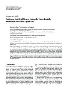
II. Problem Definition An intelligent system for airfoil shape optimization is proposed. An optimization approach with a surrogate model to approximate airfoil aerodynamics is presented. The sub-systems need to incorporate design flexibility and must be independently validated (top chart in Fig. 1), prior to application for shape optimization (bottom chart in Fig. 1). The validation process of the PARSEC shape function was tested by measuring the flexibility and accuracy of the model over a series of airfoil planforms.21 Definition of design variables is required to complete the validation process (Sec. III). The XFOIL flow solver is applied due to 2 American Institute of Aeronautics and Astronautics

rapid computation, at this preliminary stage and validated extensively in the literature. The PARSEC airfoil design variables and the corresponding aerodynamic coefficient from XFOIL are used as inputs and outputs respectively, for ANN development and validation (Sec. V). The proposed swarm algorithm also requires validation, over a series of mathematical benchmark functions. The optimizer is validated separately (Sec. IV) and not included within the airfoil shape function, flow solver and ANN test validation set-up. In the context of airfoil shape optimization, following the validation process, the flow solver is decoupled from the architecture and the validated swarm algorithm is integrated with the trained ANN database which approximates the aerodynamic coefficients. The information is used by PSO to guide the search agents towards a global solution (bottom chart in Fig. 1). Application of PSO with ANN for airfoil shape optimization is not addressed in this paper.

Figure 1. Validation and Application of Optimization Components for Airfoil Shape Optimization

III. Airfoil Shape Function – Design Variables Definition 22

The PARSEC methodology is a 6th order polynomial (Eq. 1) and used in airfoil design optimisation.5, The function is governed by eleven parameters to generate different classes of airfoils (Fig. 2) and is mathematically represented as follows: 8, 23, 24

6

z PARSEC ( x / c) =

∑a

n .x

n −1 / 2

n =1

(1)

Where: an = Real coefficients which are solved directly based on the eleven PARSEC design parameters. The coefficients an, are related to airfoil geometry. A system of equations are used to equate the coefficients as a function of variables and solved simultaneously. Variable ∆Z TE , controls the trailing edge thickness and is set to zero. Thus, blunt trailing edge sections are not considered and design variable population size is reduced to ten. The optimizer perturbs the geometrical variables to Figure 2. PARSEC Airfoil generate different classes of airfoils, until a convergence criterion is satisfied. PARSEC Design Variables Sensitivity Analysis The PARSEC variables are independently tested to verify the sensitivity of each variable on airfoil geometry and aerodynamics. The steps undertaken in the sensitivity study are as follows:
Generate base PARSEC airfoils with arbitrarily defined variables;
Select one PARSEC variable for sensitivity analysis (e.g. leading edge radius, rle) with the remaining ten variables static;
Establish variable test domain (e.g. rle test domain [0.01min - 0.04max]);
Establish variable perturbation magnitude within the test domain (e.g. rle test increments = 0.001);
Generate a series of PARSEC airfoils within the identified test domain with incremental variable changes; 3 American Institute of Aeronautics and Astronautics


Measure airfoil geometry (Leading Edge Radius, Maximum Thickness, Maximum Thickness Location, Camber, Camber Location and Trailing Edge Wedge Angle);
Evaluate the aerodynamic coefficients of lift, drag and moment of each PARSEC airfoil;
Use the initially generated planform and repeat the above till all ten variables have been independently tested; and
Repeat test with variations over four independent base airfoils Self-Organizing Maps for Data Visualization A data-mining technique was applied to visualize the processed information. Clustering SOM technique (two dimensional charts), developed by Teuvo Kohonen25 are based on the technique of unsupervised neural networks that can classify, organize and visualize large sets of data.24 The concept behind SOMs is to project n-dimensional input data into a two-dimensional map for interpretation. Each input data, in this case is the airfoil geometry variable which act as inputs or neurons to SOM architecture. The corresponding measured planform geometry and aerodynamic coefficients are outputs which are separately mapped for quick visualization on two dimensional charts based on the aforementioned test set-up. Thus, the effect of PARSEC airfoil design variable on geometry and aerodynamics is interpreted, by reducing the results from high-to-low dimensional space. SOM Results – PARSEC Airfoil Variable Definition A series of SOM charts are presented in this section to illustrate the relationship between the PARSEC variable and its effect on airfoil geometry and aerodynamics. The four base PARSEC airfoils and the specified test domain is summarized in Table 1 and presented in Figure 3. The airfoils are with varying geometrical features, to visualize the effect of applying incremental perturbations across different classes of airfoils (Fig. 3). Table 1. PARSEC Airfoil Design Variable Definition Test Case Study PARSEC Variable rle yte teg tew xu yu yxxu xl yl yxxl

Test Domain [0.01 : 0.04] [-0.02 : 0.02] [-2.0° : -25°] [3.0° : 40°] [0.30 : 0.60] [0.07 : 0.12] [-1.0 : 0.2] [0.20 : 0.60] [-0.02 : -0.08] [0.2 : 1.20]

Case 1 0.01 0 0 17° 0.3 0.06 -0.45 0.3 -0.06 0.45

Case 2 0.01 0 -6.8° 8.07° 0.4324 0.063 -0.4363 0.3438 -0.059 0.70

Case 3 0.01 0 -10° 5.6° 0.42 0.058 -0.35 0.36 -0.057 0.03

4 American Institute of Aeronautics and Astronautics

Case 4 0.01 -0.004 -10.5° 4.4° 0.418 0.055 -0.22 0.4182 -0.082 -0.35

Definition of PARSEC Variables: Case Two

Definition of PARSEC Variables: Case One

0.2

0.2 r = 0.01; y = 0; t le

te

eg

= 0; t = 17°; x = 0.3; y = 0.06; y ew

u

u

= -0.45; x = 0.3; y = -0.06; y = 0.45

xxu

l

l

le

te

eg

= -6.8 °; t = 8.07 °; x = 0.4324; y = 0.063; y = -0.4363; ew u u xxu x = 0.3438; y = -0.0589; y = 0.7 l

0.1

0.1

0.05

0.05

0

l

0

-0.1

-0.1

-0.15

-0.15

0.1

0.2

0.3

0.4

0.5 x/c

0.6

0.7

0.8

0.9

-0.2 0

1

0.1

0.2

0.3

0.4

Case 1 Definition of PARSEC Variables: Case Three

0.6

0.7

0.8

0.9

1

Definition of PARSEC Variables: Case Four 0.2

r = 0.01; y = 0; t le

0.15

= -10°; t = 5.6°; x = 0.42; y = 0.058; y = -0.35; eg ew u u xxu x = 0.36; y = -0.057; y = 0.03

te

l

l

0.15

l

0.1

0.1

0.05

0.05

0

-0.05

-0.1

-0.1

-0.15

-0.15

0.2

0.3

0.4

0.5 x/c

0.6

0.7

0.8

0.9

1

l

xxl

0

-0.05

0.1

r = 0.01; y = -0.004; t = -10.5°; t = 4.4°; x = 0.418; y = 0.055; y = -0.22; le te eg ew u u xxu x = 0.4182; y = -0.082; y = 0.3465

xxl

y/c

y/c

0.5 x/c

Case 2

0.2

-0.2 0

xxl

-0.05

-0.05

-0.2 0

r = 0.01; y = 0; t

0.15

xxl

y/c

y/c

0.15

-0.2 0

0.1

0.2

Case 3

0.3

0.4

0.5 x/c

0.6

0.7

0.8

0.9

1

Case 4

Figure 3. Base Airfoils for PARSEC Airfoil Definition
Variations in Leading Edge Radius Effect of varying rle, across the four case studies (Fig. 3) on airfoil geometry, is presented in Figure 4. The remaining nine variables are static and a change in airfoil geometry with independent PARSEC variable perturbations was recorded. Each cluster in Figure 4 represents the individual test case airfoils of Figure 3. rle

(a)

Thickness-to-Chord

(b)

Camber

Trailing Edge Wedge Angle

(c)

(d)

Figure 4. Effect of Varying rle on Airfoil Geometry The resulting airfoil geometry with leading edge radius variations is easily identifiable through the SOM charts (Fig. 4a to 4d). The minimum and maximum values of rle are denoted by ‘cold’ and ‘hot’ regions respectively for each case in Figure 4a. An increase in rle, has a negligible effect on thickness-tochord, and trailing edge wedge angle, with slight variations in camber for airfoil case two (Fig. 4b to 4d). As required, one-to-one control over thickness-to-chord, camber, and trailing edge wedge angle is permissible with variations in leading edge radius for PARSEC airfoils. The analysis confirmed that radius perturbations will not affect planform thickness, which is a key design constraint based on structural strength and payload volume necessities.

5 American Institute of Aeronautics and Astronautics

rle

Lift Coefficient

(a)

Drag Coefficient

(b)

Moment Coefficient

(c)

(d)

Figure 5. Effect of Varying rle on Airfoil Aerodynamics The equating aerodynamic SOMs are presented in Figure 5. XFOIL was applied to compute the coefficients at an operating Reynolds Number of 6.0 million at Mach 0.40. The leading edge radius has a major influence on Cl and Cd (Fig. 5b to 5c), but a minor effect on the moment coefficient (Fig. 5d). Optimization of the leading edge radius is crucial for improved drag performance. Increases in rle, cause an increase in lift and drag. These results are in-line with established airfoil aerodynamic knowledge and are confirmed by Jeong,24 where a similar analysis was performed at transonic conditions.24 It was confirmed that airfoil geometry was not influenced by rle perturbations (Fig.4) thus, rle search dimension in future optimization studies will be limited to small values for improved drag performance.
Variations in yu Similarly the effect of varying yu which provides thickness control is presented in Figure 6. The analysis shows that thickness-to-chord and camber increase proportionally as yu increases (Fig. 6b to 6c) with the trailing edge wedge angle remaining unaffected (Fig. 6d) across the four test cases (Table 1 & Fig. 3). A repeat of the analysis for PARSEC variable yl, which controls the thickness contour on the pressure side of the airfoil, indicated similar behavior. The results demonstrate variations in yu and yl exhibit one-to-one thickness control which is a key requirement for an airfoil shape function. By coupling the two control parameters, thickness constrain is imposed on the geometry through variable manipulation, for an airfoil shape optimization problem. Thus, the final optimal shape will conform to user-defined thickness requirements. yu Thickness-to-Chord Camber Trailing Edge Wedge Angle

(a)

(b)

(c)

(d)

Figure 6. Effect of Varying yu on Airfoil Geometry Aerodynamic performance with yu variations is presented in Figure 7. In general variations in yu coincide with established knowledge of airfoil aerodynamic performance of thick sections. The lift and drag coefficient rise, as airfoil thickness is increased (Fig. 7b to 7c). Airfoil aerodynamic analysis indicates delay in the onset of stall, with the maximum lift coefficient rising as airfoil thickness is increased. Smaller values of yu are related to acceptable lift-to-drag performance. With thickness constraints imposed on the model, the requirement of a robust optimization search model, for efficiently examining potential solutions within the identified thickness search limits is required. yu

(a)

Lift Coefficient

(b)

Drag Coefficient

Moment Coefficient

(c)

Figure 7. Effect of Varying yu on Airfoil Aerodynamics 6 American Institute of Aeronautics and Astronautics

(d)


Summary of SOM Analysis The goal of utilizing SOMs for PARSEC airfoil definition is not to locate an optimum planform, but to obtain an insight into the cluster structure of the data. The technique provides vital information with regards to the sensitivity of the variables. The SOM mapping analysis was simulated over the ten PARSEC design coefficients and the relationship between variable, airfoil geometry and aerodynamics mapped. The entire set of SOM charts for each design variable is not presented in this paper. The analysis indicated that the shape variables provide one-to-one geometrical control as required from a shape parameterization method. The sensitivity of the design parameters was confirmed from the mapping analysis. Parameters xu and xl which control the chord-wise location of the maximum thickness point on upper and lower surfaces, are sensitive and need to be set accordingly to mitigate un-realistic airfoil geometries. Design values within a threshold 0.20 ≤ xu ≤ 0.60 for upper and 0.20 ≤ xl ≤ 0.70 for lower contours, constitute ‘realistic’ surfaces. The function loses one-to-one geometrical control of the respective design parameter outside of the identified range, due to the generation of undulating airfoils. This information is applied in the formulation of search limits and constraints during an optimization run to mitigate airfoils that are aerodynamically and geometrically unfeasible. The aerodynamic convergence data identified the influence of design coefficients on the aerodynamic properties of airfoils. It is evident that design coefficients with acceptable drag may not offer the required lift performance. Thus, a design compromise is necessary and the development of an intelligent search agent to address this issue needs to be the design focus.

IV. Airfoil Shape Optimization – Intelligent Search Agent Validation In this section, the search agent used for airfoil optimization is introduced and validated. The algorithm is tested over a series of benchmark functions, to determine the sensitivity of the model for convergence. SOMs are used to qualitatively show the results of the validation process. The maps illustrate the relationship between variables that control the search process, and the effect on solution convergence. From the charts, the set-up of the search model with robust convergence across the test envelope is established. A. Particle Swarm Optimizer A global seeking search agent capable of handling multi-objective problems is identified for this study. The PSO method, first developed by Eberhart and Kennedy26 evolves from the paradigm of swarm of birds. The method provides a simple and efficient architecture and is ideal for continuous variable problems. Consequently, the algorithm has been applied across various optimization disciplines.27 The methodology is similar to evolutionary programming techniques, with the population initialized through random dispersion of particles. Each particle maintains a personal record of its position, thus fitness from an optimization perspective. An information sharing methodology is initiated within the swarm to guide the remaining particles towards the group leader. Over time the particles reach a consensus and settle onto the final destination to provide an optimal solution. Each particle in swarm of size ‘m’, is a potential solution of the objective function and is represented by the relative position ' xi ' and velocity ' vi ' . The velocity rate of change (Eq. 3) is a function of user predefined learning factors as follows: a) Cognitive c1 ; and b) Social c 2 parameters that influence local and global

search

patterns.

At

each

iteration

the

position [ xi = ( x i1, xi 2,..., xin ), i = 1,2,..., m]

and

velocity [vi = (v i1, vi 2,..., vin ), i = 1,2,..., m] of the individual particles is recorded and solution fitness evaluated and stored [ Pgbest = ( Pg1, Pg 2,..., Pgn )]. A particle with the ‘best’ global solution, ' Pgbest ' , from the population, is recorded and the remaining particles update their position and velocity to follow Pgbest over the subsequent iterations until solution convergence.27 At each iteration ' k ' , the search direction is refined by updating the position, ' xi (k + 1)' , and velocity, ' vi (k + 1)' , (Eqs. 2 & 3) of the particles, with convergence occurring when all particles are within a set threshold of each other. The PSO algorithm has been adequately modified with the aim of implementing a robust model to be applied across various optimization problems.1, 28-30 The two variants tested in this study are as follows: a) Standard-PSO (SPSO) algorithim;29 and b) Adaptive Inertia Weight (APSO)1 model - Table 2. APSO was introduced to add greater search flexibility in comparison to the SPSO algorithm and to address the shortfalls of the standard search model.

7 American Institute of Aeronautics and Astronautics

The PSO requires user inputs to define the search parameters. In the two variants (SPSO and APSO), social and cognitive parameters are set to c1 = c 2 = 2 and have been successfully applied in previous optimization studies.1, 27 The inertia weight factor ‘w’, which provides a balance between local and global search patterns, is constant throughout the iteration run (Eq. 4) for the SPSO and is a function of userdefined learning factors.29 Thus, social and cognitive parameters need to be set accordingly to influence the search behavior and is challenging to set. A new method of calculating w, was proposed by Qin. et. al1 , referred to as the APSO where w, is dynamically calculated at each iteration.1 The position of each particle within the swarm, including individual and overall global ideal solution (Eq. 5)1 is considered in the calculation of w within the APSO scheme (Eq. 6).1 At each iteration the behavior of the swarm is established and w modified, to adapt the model with the current search region. Theoretically, this methodology permits global search capabilities at the start of the PSO run with large values of w, which dampen into smaller values as the search region narrows.

xi (k + 1) = xi (k ) + vi (k + 1) vi (k + 1) = w.vi (k ) + c1 .rand .( Pi − xi (k )) + c 2 .rand .( Pg − x i (k )) w=

2 2 − ϕ − ϕ 2 − 4ϕ

(2) (3)

; where ϕ = c1 + c 2 = 4

Individual Search Ability (ISA): ISAij =

(4)29

xij − pij

(5)1

pij − p gj + ε

  1 ; where α is in the range (0,1] wij = 1 − α  (6)1 − ISAij  1+ e  The effect of varying the maximum velocity of the particles across both the SPSO and APSO scheme is further examined in the validation run. If the maximum velocity of the particles is too high, the particles overshoot the dimensional space and the global minimum. This causes solution oscillations thus, increasing the number of iterations required for convergence. The application of wall boundary conditions will be required to re-instate the particles back into the search domain. To mitigate this requirement, the maximum velocity of the particles was examined in the range 0.1% - 10% of the maximum dimensional search space ' λ max ' , for each variable. The two PSO models examined in the validation study is summarised in Table 2: Table 2. Particle Swarm Optimizer: Model Variants for Validation SPSO

APSO1

c1 = 2

c1 = 2

c2 = 2

c2 = 2

Swarm Population (m)

20,40 & 80

20,40 & 80

Number of Dimensions (D)

10,20 & 30

10,20 & 30

Maximum Iterations

1000,1500 & 2000

1000,1500 & 2000

PSO Model Scaling Learning Factors

Cognitive & Social (c1 & c2)

w=

2

;

ISAij =

2 − ϕ − ϕ 2 − 4ϕ

Inertia Weight (w)

where ϕ = c1 + c 2 = 4 Maximum Velocity (Vmax)

0.1 – 10% of λ1 max , … , λ n max

xij − pij pij − pgj + ε

 1 wij = 1 − α  − ISAij 1+ e

 ; where α = 0.3  

0.1 – 10% of λ1max , … , λn max

8 American Institute of Aeronautics and Astronautics

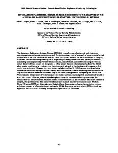
B. Optimizer Validation Two mathematical functions (Fig. 8 to 9) are applied in the validation process. The objective (Eq. 7) is to use the two PSO models (Table 2), to locate the global minimum of the functions (Eqs. 8-9) Objective Function: f (x) min (7) Rosenbrock Function:

Schwefel Function:

n −1

f ( x) =

∑

n

[100( xi2 − xi +1 ) 2 + ( xi − 1)2 ]

f ( x) = 418.9829n −

(8)

i =1

∑ ( x sin i

xi )

(9)

i =1

Figure 8: Test Function One: Rosenbrock Function

Figure 9: Test Function Two: Schwefel Function

The search parameters and the theoretical solution of the functions, is summarized in Table 3.

Table 3. PSO Set-Up for Test Function Evaluation and Summary of Theoretical Solution

Rosenbrock

Dimension Search Space (λ1,2,...,n) −100 ≤ x i ≤ 100, i = 1,2, … , n

Particle Initialization Range 15 ≤ x i ≤ 30

X * = (1, ⋯ ,1), f ( x * ) = 0

Schwefel

−500 ≤ x i ≤ 500, i = 1,2, … , n

250 ≤ x i ≤ 500

X * = (1, ⋯ ,1), f ( x * ) = 0

Function

Global Minima (Theoretical Solution)

C. Validation Results and Visualization
Rosenbrock Function A series of SOM charts are applied to represent the results of the validation process. The fitness convergence for SPSO (Fig. 10b) and APSO (Fig. 10c), with variations in Vmax (Fig. 10a) as a percentage of search space (Table 3), over the number of dimensions D (Table 2), is represented by each cluster separator in Figure 10. Low Velocity = Low Fitness Velocity

SPSO

Vmax as a % of λmax (a) Figure 10.

APSO

Fitness Fitness (b) (c) Rosenbrock Function Convergence: SOM Visualization

9 American Institute of Aeronautics and Astronautics

The SOM charts (Fig. 10a to 10c) indicate that low velocity equates to low fitness for both SPSO and APSO. This is evident across the entire test domain where an increase in D, equates to an increase in fitness. It is thus established, that particles need to navigate about the solution space at slow speeds to converge. Faster moving particles mitigate global minima regions by overshooting key areas of interest. Direct comparison between SPSO and APSO (Fig. 10b to 10c) indicates that the APSO provides superior convergence across the evaluated testing domain in comparison to the SPSO model (Fig. 10b). In all tests, the termination criterion is based on the maximum iteration count (Table 2). It is evident from the charts, that SPSO and APSO are not capable of converging to the theoretical solution based on the formulated termination criteria. In general SPSO indicates greater areas of ‘hot’ regions in ‘red’ shade referring to higher fitness. The APSO evolution, at the same operating conditions, consists of larger ‘cold’ regions in ‘dark blue’ shade, thus indicating that the APSO map consists of lower fitness in comparison, across the testing domain. Thus, comparison between SPSO and APSO (Fig. 10b to 10c) confirms that a linear decreasing inertia weight, where a global search process is enabled at the start of the search phase and local, during the later stages provides acceptable solution convergence. A fixed inertia weight causes solution convergence instabilities, as the search pattern (global vs. local) does not adapt during the search phase. The relationship between particle population (m = 20, 40, 80) and velocity as a function of fitness is represented in Figure 11. Higher particle population (m = 80), with the velocity restricted to approximately 0.1% of λ1 max to λ n max , indicates low fitness. At the same speed, with fewer particles (m = 20), fitness increases by 4% in comparison. It is observed from the test, that greater number of particles is required to assist convergence. The fitness presented here is compared with the findings reported by Z. Qin et al.1 with their AIWPSO model.1 Essentially the APSO used in Figure 11. Rosenbrock Function: Effect of this study is the model developed by Z. Qin et Varying Particle Population & Velocity on Fitness al.1 with the exception being in the treatment of the maximum velocity. Essentially Z. Qin et al.1 fixed Vmax equal to the maximum distance of each dimension.1 In this study, we examined the effect of varying Vmax for both models (Table 2) on solution convergence. Table 4 presents fitness comparisons between the SPSO, APSO and Z. Qin et al.1 AIWPSO model, with the data taken directly from literature.1 The SPSO and APSO data (Table 4), equates to a velocity threshold of 0.1% of λ max , as this condition was proven to be most effective (Fig. 10 to Fig. 11). Comparing the SPSO with AIWPSO model, it is seen that in most conditions, the SPSO model yields lower fitness. Thus, the benefits associated with a linearly decreasing inertia weight, within the AIWPSO model does not provide the expected search benefits, as this is counteracted by the higher particle velocity. The SPSO model, which has a fixed inertia weight at lower velocities, outperforms a model with an adaptive inertia weight with higher velocities. Thus, the importance of correctly setting the maximum allowable velocity, on solution convergence is re-enforced. Comparisons between the APSO and AIWPSO model, indicates that the APSO provides superior convergence across the examined test domain, due to particle simulation at a lower velocity. Comparing the SPSO and APSO, it is evident that the adaptive inertia weight scheme clearly outperforms a model with fixed inertia weight, associated with the SPSO model.

10 American Institute of Aeronautics and Astronautics

Table 4. Rosenbrock Function: Fitness Evaluation Comparison through different PSO Model Population Size

Dim

20

10 20 30 10 20 30 10 20 30

40

80

a

Max. Iteration 1000 1500 2000 1000 1500 2000 1000 1500 2000

SPSO

APSO

AIWPSO1

34.4393 92.4618 156.8884 18.0475 85.2453 129.5636 13.2744 79.2820 100.9905

17.1394 17.3522 19.1374 17.2192 16.7663 18.8235 17.8872 17.9988 18.3088

48.6378 115.1627 218.9012 24.5149 60.0686 128.7677 19.2232 52.8523 149.4491

Bold face indicates the best result in the respective PSO variant test run


Schwefel Function The Schwefel function, the second model applied for optimizer validation indicated similar results. It was observed that an optimum velocity of 0.1% of λ max , provided a theoretical fitness of zero. Solution convergence towards the theoretical minima was accelerated with a larger particle population. The position of the particles (Eq. 2), thus solution is dependent on the velocity (Eq. 3). By restricting the maximum speed, the probability of the particles overshooting a global solution over successive iterations is minimized thus, assisting convergence.

V. Artificial Neural Networks The DNO process is computationally time demanding, especially if Navier-Stokes solvers are integrated for aerodynamic computation. PSO validation indicated the requirement for large number of particles to support convergence. A DNO simulation for single-point airfoil design analysis was attempted.31 The optimizer examined in excess of 2000 airfoils before converging to an optimal planform.31 With the integration of panel method solvers, computational time was negligible. By replacing low fidelity solver with NavierStokes model for solution accuracy, the computational time is excessive, thus the use of ANN is proposed to address this issue. Figure 12. PARSEC Airfoil Artificial Neural Network Structure It is hypothesized that a trained network, when integrated to a DNO structure, will significantly reduce the computation expense of airfoil shape optimization. The network will de-couple the solver from the DNO process, with the swarm algorithm operating simultaneously with the neural network. The technique was successfully applied in the design of single15 and multi-element airfoils,10 including the design of turbomachinery sections11 and in the minimisation of wind tunnel data for aerodynamic performance evaluation.14 In this study, an ANN structure is introduced (Fig. 12), to develop a relationship between PARSEC airfoil shape variables as inputs and the equating aerodynamic coefficient as output.


Neural Network Training and System Generalization The network training data consisted of 3000 PARSEC airfoils generated by Latin Hypercube Sampling (LHS). A training dataset with LHS methodology guarantees acceptable, uniform distribution for the proposed solution space. A requirement of neural network is to provide acceptable generalization performance with minimal training dataset. The LHS methodology for training dataset distribution provides an acceptable framework to address this requirement. A batch training process with Bayesian regularization by MacKay,32 and the combination of Levenberg11 American Institute of Aeronautics and Astronautics

Marquardt training algorithm is used to train the network. The aerodynamic computations for network development and validation were simulated at a Reynolds and Mach number of 3.0 million and 0.35 respectively at an angle-of-attack of zero degrees. The training goal for convergence was set with one of the following conditions:
Network Training Error - Zero Sum-Square-Error between theoretical and network computed lift coefficient; or
Overfitting - When network exhibits over-fitting of training data over a succession of 50 training iterations In total ten networks with different combinatorial experiments were conducted with the following network structure variations:
Data Preprocessing – To improve network efficiency, inputs and outputs were scaled within a specified range. Two normalization techniques were tested:  Normalizing data in the range [-1,1]; and  Normalizing data to have a mean of zero and unity standard deviation
Number of Hidden Layers – Variation in the size of hidden layers was tested; and
Transfer Functions – Order of sequence of transfer functions within the hidden layers with variations in tan-sigmoid and log-sigmoid functions. Linear function used to model the output data A minimum number of 50 neurons were evaluated within the hidden layers. This is based on a thumb-of-rule assumption that the number of neurons in the hidden layer equals five times the number of input neurons (ten PARSEC variables). The assumption was proven reasonable by Rajkumar et. al. in the prediction of lateral and longitudinal aerodynamic forces using neural networks.20 Results with variations in network architecture for two networks, with acceptable convergence based on the measure of R-Square correlation value for 1000 generalization airfoils is presented in Table 5.

Table 5. Neural Network Configuration for PARSEC Airfoils Lift Coefficient Prediction Model

ANN Architecture

1

10-60-50-1

2

10-50-50-1

Transfer Function Input Hidden Hidden Output

Training Algorithm Bayesian Regularization with LM Bayesian Regularization with LM

Training Dataset

Generalization Dataset

R-Square

tansig

tansig

3000

1000

0.97

tansig

logsig

3000

1000

0.98

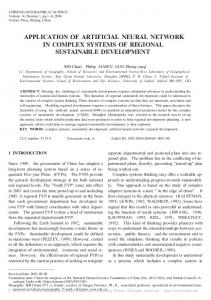
The two networks exhibit similar performance based on the R-Correlation measure from network generalization simulation (Table 5). The response of the models is presented by performing a regression analysis between network response and the corresponding targets (Fig. 13). The network outputs are plotted versus the targets (open circle data points) and the best linear fit, through the data is indicated by the ‘dashed’ line. The correlation between network and target data is indicated by a ‘solid’ line (Fig. 13). The charts (Fig. 13a & Fig. 13b) for the two networks, indicates acceptable linear fit. Model 2 exhibits a higher R-Correlation of 0.98 in comparison to 0.97 for Model 1 (Table 5 and Fig. 13). Best Linear Fit: A = (0.956) T + (0.0144)

Best Linear Fit: A = (0.958) T + (0.0146)

1

1 R = 0.98

0.8

0.8

0.6

0.6

0.4

0.4

A

A

R = 0.97

0.2

0.2

0

Data Points

Data Points

0

Best Linear Fit

Best Linear Fit

A=T

A=T -0.2 -0.2

0

0.2

0.4

0.6

0.8

-0.2 -0.2

0

0.2

T

0.4

0.6

0.8

T

(a) Model 1: Network Generalization Regression Analysis 10-60-50-1; tansig - tansig

(b) Model 2: Network Generalization Regression Analysis 10-50-50-1; tansig – logsig

Figure 13. Neural Network Regression Analysis for PARSEC Airfoils Lift Coefficient Prediction

12 American Institute of Aeronautics and Astronautics

The R-Correlation value is further defined against the proposed network output - coefficient of lift over the generalization population data. A summary of network results, based on the measure of percentage difference between network output and theoretical data, over a testing envelope of 1000 airfoils of the two models is presented in Table 6.

Table 6. Neural Network Configuration for PARSEC Airfoils Lift Coefficient Summary of Errors Model 1 2

ANN Architecture 10-60-50-1 10-50-50-1

Min. % Error 0 0

Max. % Error 1766 294

Average % Error 15.32 12.46

Theoretically, an R-Correlation value of 0.98 indicates an excellent fit between two datasets. The measure is analysed as function of aerodynamic lift approximation of PARSEC airfoils from neural network simulations. A percentage error of approximately 15% between network output and theoretical solution over the tested population of 1000 airfoils is evaluated for Model one, compared to 12% for second model. Both models contained samples where the predicted lift represented the theoretical solution, thus a minimum percentage error of zero (Table 6). Maximum percentage difference in the two models is large (Table 6). This corresponds to a point were the theoretical lift coefficient is close to zero and the network fails to adequately simulate data at this region. A histogram analysis of the two models, to illustrate the frequency airfoils, belonging to several groups of percentage error categories is presented in Figure 14.

600

500

400

300

200

100

0 0

Histogram of Coefficient of Lift Percentage Error for Neural Network PARSEC Airfoil Simulations 700

Frequency of Neural Network Simulation Airfoils

Frequency of Neural Network Simulation Airfoils

Histogram of Coefficient of Lift Percentage Error for Neural Network PARSEC Airfoil Simulations 700

200

400

600

800 1000 Percentage Error

1200

(a) Model 1 Figure 14.

1400

1600

1800

600

500

400

300

200

100

0 0

50

100

150 Percentage Error

200

250

300

(b) Model 2 Histogram of Percentage Errors

The percentage error histogram is in intervals of 10% (Fig. 14) and distributed evenly in the two charts (Fig. 14a & 14b) for ease of comparison. Most airfoils are in interval one for the two models thus, representing an error of 0% - 10% between network simulation and theoretical data. Model one simulates 70% of airfoils out of the total 1000 with an error less than 10% compared to 68% for Model two. Over the first two intervals, relating to a percentage error of 0% - 20%, network one models 83% of airfoils compared to 82% for Model two. Thus, over the first two intervals, the two networks (Table 6) present similar performance. The difference between the two models is in scatter of data, in particular the presence of outliers defined as 1.5 × Inter - Quartile - Range . Model one contains 104 outliers compared to 94 for Model two. Percentage errors in excess of 800% are present for the extreme most outliers in Model one, compared to 294% in Model two. The excessively high percentage errors within the outliers in Model one result in a higher mean error percentage in comparison to Model two. It is evident from the analysis, that the neural network methodology is suitable for the proposed architecture (Fig. 12). Percentage errors greater than 10% are considered excessive and approximately 30% of airfoils (300 out of 1000) exceeded this threshold in Model two, which is optimal from the initial ten networks developed and tested in this study. Thus, the neural network requires design modifications to further reduce the percentage error and the scatter of data, in particular the presence of extreme outliers. At this stage, the training dataset was fixed to 3000 airfoils with the size dependent on the available computing hardware. Further increases in training population demand greater computing memory. Thus, alternate 13 American Institute of Aeronautics and Astronautics

training algorithms and/or computer hardware that support the required memory requirements, need to be explored to address this constraint.

VI. Conclusion and Future Work The DNO approach for airfoil design and analysis was introduced. A study to independently validate the components within the DNO architecture was proposed. A data mining technique, through SOM charts was applied to project multi-dimensional output data, into two dimensional maps for results visualization. Within the overall DNO structure, the following components were validated for eventual integration in airfoil design optimization architecture:
Definition of PARSEC shape function design variables;
Validation of the PSO model; and
Design and validation of an ANN structure to model the lift coefficient The behavior of the design variables within the PARSEC function was defined. A series of PARSEC airfoils were generated (Fig. 3) and periodic perturbations applied to each variable to study the effect on airfoil geometry and aerodynamics. It was proved that variables provide one-to-one geometrical control which is a key requirement for a parameterization technique, such that shape constraints can be imposed. All variables are operational up to an identified threshold, beyond which un-realistic shapes are generated. This further assists in the development of search limits of the PARSEC coefficients for detail design optimization routines. Aerodynamically, the effect of variable perturbations on airfoil performance was mapped, with the findings conforming to established aerodynamic knowledge. The variable definition process provided an indication as to the expected behavior of each variable, and the design limits under which these variables can operate. Consequently, geometrical constraints through each of these variables can be imposed and the search limits defined with confidence, to mitigate the optimizer searching for airfoils that are geometrically and aerodynamically unfeasible. A PSO search agent was proposed with two variants tested. A series of simulations over two benchmark functions was undertaken to determine the suitability of each model. The effect of varying particle population and velocity across multiple dimensions, on convergence towards the theoretical solution was examined. The results were mapped onto a series of SOM charts, which indicated that the adaptive inertia weight model was superior in comparison to a standard PSO algorithm. Large particle population with low velocities provides acceptable convergence in comparison to an optimization run with fewer particles navigating at faster speeds. Current research focuses on developing an adaptive inertia velocity function, similar to the inertia weight model, to adapt the speed of the particles through a PSO run. This has the potential of providing greater solution agreement with fewer design iterations. The ANN methodology within the overall DNO framework was introduced. The PARSEC design variables were used as inputs, with the lift coefficient as output to the system (Fig. 12). Preliminary results indicate that the proposed methodology is suitable for design application within the DNO structure. The model proposed requires further design, development and validation to reduce the simulation percentage errors. Current research focuses on increasing the training dataset of the network, with the aim of simulating output data that represents the theoretical solution with minimal percentage difference. Network development to simulate drag and moment coefficients is also a present research activity.

Acknowledgment Bernhard Kuchinka – Viscovery Software GmbH, Vienna, Austria, for kindly offering a free copy of SOMine 4.0 for the duration of this research. Markus Trenker - Arsenal Research, Austria for his assistance in developing the PARSEC airfoil geometry code.

References 1

Qin, Z., Yu, F., Shi, Z. and Wang, Y., "Adaptive Inertia Weight Particle Swarm Optimization," ICAISC, 2006, pp. 450-459. 2 Besnard, E., et al., "Hydrofoil Design and Optimization for Fast Ships," ASME International Congress and Exhibition, Anaheim, CA, 1998, pp. 11. 3 Prouty, R. W., Helicopter Performance, Stability and Control, Krieger Publishing Company, Inc., Malabar, Florida, 1995.

14 American Institute of Aeronautics and Astronautics

4 Gallart, M. S., "Development of a Design Tool for Aerodynamic Shape Optimization of Airfoils," Master of Applied Science, Department of Mechanical Engineering, University of Victoria, 2002. 5 Fuhrmann, H., "Design Optimisation of a Class of Low Reynolds, High Mach Number Airfoils For Use in the Martian Atmosphere," 23rd AIAA Applied Aerodynamics Conference, 2005. 6 Namgoong, H., "Airfoil Optimization of Morphing Aircraft," PhD, Aerospace Engineering, Purdue, Indiana, 2005. 7 Holst, T. L. and Pulliam, T. H., "Aerodynamic Shape Optimization Using a Real-Number-Encoded Genetic Algorithm," NASA, 2001. 8 Winnemoller, T. and Dam, C. P. V., "Design and Numerical Optimization of Thick Airfoils," 44th AIAA Aerospace Sciences Meeting and Exhibit, 2006, pp. 1-14. 9 Quagliarella, D. and Vicini, A., "Viscous single and multicomponent airfoil design with genetic algorithms," Finite Elements in Analysis and Design, 2001, pp. 365-380. 10 Greenman, R. M. and Roth, K. R., "Minimizing Computational Data Requirements for Multi-Element Airfoils Using Neural Networks," Journal of Aircraft, Vol. 36, No. 5, 1999, pp. 777-784. 11 Rai, M. M. and Madavan, N. K., "Application of Artificial Neural Networks to the Design of Turbomachinery Airfoils," 36th Aerospace Sciences Meeting & Exhibit, Reno, NV, 1998, 12 D'Angelo, S. and Minisci, E., "Multi-Objective Evolutionary Optimization of Subsonic Airfoils By MetaModeling and Evolution Control," Proceedings of the Institution of Mechanical Engineers, Part G: Journal of Aerospace Engineering, Vol. 221, No. 5, 2007, pp. 805-814. 13 Rai, M. M. and Madavan, N. K., "Aerodynamic Design Using Neural Networks," AIAA Journal, Vol. 38, No. 1, 2000, pp. 173-182. 14 Ross, J. C., Jorgenson, C. C. and Norgaard, M., "Reducing Wind Tunnel Data Requirements Using Neural Networks," NASA Technical Memorandum, 1997. 15 Hacioglu, A., "Fast Evolutionary Algorithm for Airfoil Design via Neural Network," AIAA Journal, Vol. 45, No. 9, 2007, pp. 2196-2202. 16 Duvigneau, R. and Visonneau, M., "Hybrid Genetic Algorithms and Neural Networks For Fast CFD-Based Design," 9th AIAA/ISSMO Symposium on Multidisciplinary Analysis and Optimization, Atlanta, Georgia, 2002, pp. 633-643. 17 Santos, M. C. d., Mattos, B. S. d. and Girardi, R. d. M., "Aerodynamic Coefficient Prediction of Airfoils Using Neural Networks," 46th AIAA Aerospace Sciences Meeting and Exhibit, Reno, Nevada, 2008, 18 Norgaard, M., Jorgensen, C. C. and Ross, J. C., "Neural Network Prediction of New Aircraft Design Coefficients," NASA Ames Research Center, 1997. 19 Huang, S. Y., Miller, L. S. and Steck, J. E., "An Exploratory Application of Neural Networks to Airfoil Design," 32nd Aerospace Sciences Meeting and Exhibit, Reno, NV, 1994, pp. 10. 20 Rajkumar, T. and Bardina, J., "Training Data Requirements for a Neural Network to Predict Aerodynamic Coefficients," Independent Component Analyses, Wavelets, and Neural Networks, Vol. 5102, Orlando, FL, USA, 2003, 21 Khurana, M., Sinha, A. K. and Winarto, H., "Multi-Mission Re-Configurable Unmanned Aerial Vehicle - Airfoil Optimisation Architecture," International Conference on Engineering Technology, Kuala Lumpur, Malaysia, 2007, pp. 10. 22 Sobieczky, H., "Parametric Airfoils and Wings," Numerical Fluid Dynamics, Vol. 68, 1998, pp. 71-88. 23 Vavalle, A. and Qin, N., "Iterative Response Surface Based Optimization Scheme for Transonic Airfoil Design," Journal of Aircraft, Vol. 44, No. 2, 2007, pp. 365-375. 24 Jeong, S., Chiba, K. and Obayashi, S., "Data Mining for Aerodynamic Design Space," Journal of Aerospace Computing, Information and Communication, Vol. 2, 2005, pp. 452-469. 25 Kohonen, T., Self-Organizing Maps, Springer, Berlin, Heidelberg, 1995. 26 Kennedy, J. and Eberhart, R., "Particle Swarm Optimization," IEEE International Conference on Neural Networks, Perth, Australia, 1995, pp. 1942-1948. 27 Robinson, J. and Rahmat-Samii, Y., "Particle Swarm Optimization in Electromagnetics," IEEE Transactions on Antennas and Propagation, Vol. 52, No. 2, 2004, pp. 397-407. 28 Eberhart, R. C. and Shi, Y., "Particle Swarm Optimization: Developments, Application, and Resources," Congress on Evolutionary Computation CEC2001, IEEE, Vol. 1, 2001, pp. 81-86. 29 Eberhart, R. C. and Shi, Y., "Comparing Inertia Weights and Constriction Factors in Particle Swarm Optimization," Congress on Evolutionary Computation, Vol. 1, 2000, pp. 84-88. 30 Zheng, Y.-l., Ma, L.-h., Zhang, L.-y. and Qian, J.-x., "Empirical Study of Particle Swarm Optimizer with an Increasing Inertia Weight," 2003, pp. 221-226. 31 Khurana, M., Sinha, A. and Winarto, H., "Multi Mission Re-Configurable UAV - Airfoil Optimisation through Swarm Approach and Low Fidelity Solver," 23rd Bristol International Unmanned Air Vehicle Systems Conference, Bristol, United Kingdom, 2008, 32 MacKay, D. J. C., "Neural Computation: Bayesian Interpolation," Neural Comput., Vol. 4, No. 3, 1992, pp. 415447.

15 American Institute of Aeronautics and Astronautics