Application of the Fuzzy Weighted Average of Fuzzy Numbers in Decision Making Models Ondˇ rej Pavlaˇ cka Department of Mathematical Analysis and Applied Mathematics, Faculty of Science, Palack´ y University Olomouc, tˇr. Svobody 26, 771 46 Olomouc, Czech Republic
[email protected]
Abstract The paper deals with the operation of fuzzy weighted average of fuzzy numbers. The operation can be applied to the aggregation of partial fuzzy evaluations in fuzzy models of multiple criteria decision making and to the computation of expected fuzzy evaluations of alternatives in discrete fuzzy-stochastic models of decision making under risk. Normalized fuzzy weights figuring in the operation have to form a special structure of fuzzy numbers; its properties will be studied and the practical procedures for setting them will be proposed. A fuzzy weighted average of fuzzy numbers with normalized fuzzy weights will be defined, an effective algorithm of its calculation will be described, and its uncertainty will be studied.
1
Jana Talaˇ sov´ a Department of Mathematical Analysis and Applied Mathematics, Faculty of Science, Palack´ y University Olomouc, tˇr. Svobody 26, 771 46 Olomouc, Czech Republic
[email protected]
resent shares of the corresponding partial objectives of evaluation in the overall one. This concept of criteria weights will be considered in this paper. The weighted average operation is applied also in the models of decision making under risk where evaluations of alternatives depend on a finite number of states of the world whose probabilities are known. The best alternative is chosen according to expected evaluations of alternatives. They are computed by means of the weighted average operation where the probabilities of states of the world play the role of weights.
Keywords: Multiple criteria decision making, decision making under risk, normalized fuzzy weights, fuzzy weighted average, fuzzy weights of criteria, fuzzy probabilities.
The weights of criteria as well as the probabilities of states of the world are usually set subjectively, i.e. they are more or less uncertain. In this paper, it will be shown how this kind of uncertain information can be expressed by means of tools of fuzzy sets theory. A special structure of fuzzy numbers, normalized fuzzy weights, will be introduced for expressing the uncertain normalized weights and the operation of the fuzzy weighted average of fuzzy numbers with normalized fuzzy weights will be defined. In the end, application of the fuzzy weighted average operation in decision making models will be shown.
Introduction
2
In multiple criteria decision making models, the weighted average is often used for aggregating partial evaluations of alternatives. Weights of criteria are understood differently in different models. The most general definition says that the weights of criteria are non-negative real numbers whose ordering expresses the importance of criteria. According to this definition, the weights mean the measurements of criteria importance that are defined on an ordinal scale. But in most of multiple criteria decision making models, the weights of criteria represent some kind of cardinal information about the importance of criteria. For example, in the model of multiple criteria evaluation that was introduced in [8] the weights of criteria rep-
Applied Notions of Fuzzy Sets Theory
In this paper, the following notation will be used. The symbol Nm denotes the index set {1, 2, . . . , m}. A fuzzy set A on a universal set X is characterized by its membership function A : X → [0, 1]. Ker A denotes the kernel of A, i.e. Ker A = {x ∈ X | A(x) = 1}. For α ∈ (0, 1], Aα denotes the α-cut of A, i.e. Aα = {x ∈ X | A(x) ≥ α}. Supp A denotes the support of A, i.e. Supp A = {x ∈ X | A(x) > 0}. A fuzzy number is a fuzzy set C on the set of all real numbers ℜ that fulfils the following conditions: a) Ker C 6= ∅, b) Cα are closed intervals for all α ∈ (0, 1], c) Supp C is a bounded set. A fuzzy number C is
said to be defined on [a, b], if Supp C ⊆ [a, b]. Let us denote [c1 , c4 ] = Cl(Supp C), [c2 , c3 ] = Ker C; Cl(Supp C) means the closure of Supp C. The real numbers c1 ≤ c2 ≤ c3 ≤ c4 are called significant values of C. A fuzzy number C can be also characterized (see [3]) by the pair of functions (c, c), both from [0, 1] to ℜ, that satisfy the following property c(α) ≤ c(β) ≤ c(β) ≤ c(α),
0 ≤ α ≤ β ≤ 1.
(1)
Calculations with fuzzy numbers are based on the extension principle (see [3]). Let f : [a1 , b1 ] × [a2 , b2 ] × . . . × [an , bn ] → ℜ be a continuous function and let f ([a1 , b1 ] × [a2 , b2 ] × . . . × [an , bn ]) = [c, d]. Let Xi be fuzzy numbers defined on [ai , bi ], for i ∈ Nn . Then f (X1 , X2 , . . . , Xn ) is a fuzzy number Y defined on [c, d] whose membership function is given as follows © Y (y) = max min{X1 (x1 ), X2 (x2 ), . . . , Xn (xn )} | ª y = f (x1 , x2 , . . . , xn ) (7)
Then, for the membership function C of the fuzzy number C = (c, c) the following holds © ª C(x) = max α | x ∈ [c(α), c(α)] (2)
for y ∈ [c, d], and 0 elsewhere. Employing the (y, y) representation of the fuzzy number Y , the following holds for any α ∈ [0, 1]
If c(α) = c = c(α), for all α ∈ [0, 1], then C represents a real number; C = c, c ∈ ℜ. A fuzzy number C is called symmetric with the central point c if the following holds
In some cases (see [5] for more details), it is necessary to consider a relation R among the variables x1 , x2 , . . . , xn . Let R be a closed and convex subset of [a1 , b1 ] × [a2 , b2 ] × . . . × [an , bn ] and let f R : R → [c, d] be the restriction of f on R. Let there exist at least one n-tuple (x1 , x2 , . . . , xn ) ∈ R such that Xi (xi ) = 1 for all i ∈ Nn . Then f R (X1 , X2 , . . . , Xn ) is a fuzzy number Y R defined on [c, d] whose membership function is given in the following way © Y R (y) = max min{X1 (x1 ), X2 (x2 ), . . . , Xn (xn )} | ª y = f (x1 , x2 , . . . , xn ), (x1 , x2 , . . . , xn ) ∈ R (9)
for x ∈ [c(0), c(0)], and 0 elsewhere; i.e. Cα = [c(α), c(α)] for all α ∈ (0, 1], Cl(Supp C) = [c(0), c(0)].
c=
c(α) + c(α) , 2
for α ∈ [0, 1].
(3)
A fuzzy number C = (c, c) is called a linear fuzzy number if both c and c are linear functions. Any linear fuzzy number C is fully characterized by its significant values c1 ≤ c2 ≤ c3 ≤ c4 ; the functions c and c are given for all α ∈ [0, 1] as follows c(α)
= c1 + α(c2 − c1 ),
c(α)
= c4 − α(c4 − c3 ).
(4)
The notation C = hc1 , c2 , c3 , c4 i is used in this paper for such a fuzzy number C. For c2 6= c3 , the linear fuzzy number C is usually referred to as a trapezoidal fuzzy number, for c2 = c3 as a triangular fuzzy number. For any fuzzy number C = (c, c), the non-increasing, non-negative function σC (α) = c(α) − c(α),
for α ∈ [0, 1],
(5)
y(α) = min{f (x1 , x2 , . . . , xn ) | xi ∈ Xiα , i ∈ Nn }, y(α) = max{f (x1 , x2 , . . . , xn ) | xi ∈ Xiα , i ∈ Nn }. (8)
for y ∈ [c, d], and 0 elsewhere. Employing the (y R , y R ) representation of the fuzzy number Y R , the following holds for any α ∈ [0, 1] © y R (α) = min f (x1 , x2 , . . . , xn ) | ª (x1 , x2 , . . . , xn ) ∈ (X1α × X2α × . . . × Xnα ) ∩ R , © y R (α) = max f (x1 , x2 , . . . , xn ) | ª (x1 , x2 , . . . , xn ) ∈ (X1α × X2α × . . . × Xnα ) ∩ R . (10)
3
Normalized Fuzzy Weights
is called a width function of C. It describes in details, for any membership degree α, the uncertainty of C. The real numbers σC (1), σC (α) and σC (0) are called the width of the kernel, the width of the α-cut and the width of the support, respectively. Obviously, σC (α) = 0 for all α ∈ [0, 1] if and only if C is a real number. It holds that Z Z 1 σC (α) dα = C(x) dx, (6)
In this section, a special structure of fuzzy numbers, normalized fuzzy weights, will be introduced, and its properties will be studied. Normalized fuzzy weights represent a fuzzification of crisp normalized weights that are defined asPnon-negative real numbers m w1 , w2 , . . . , wm such that i=1 wi = 1.
where the right-hand side of the equation represents the usual aggregated measure of uncertainty of the fuzzy number C.
For any wi ∈ Wiα there exist wj ∈ Wjα , j ∈ Nm , m P wj = 1. (11) j 6= i, such that wi +
0
ℜ
Fuzzy numbers W1 , W2 , . . . , Wm defined on [0, 1] are called normalized fuzzy weights if for any α ∈ (0, 1] and for all i ∈ Nm the following holds:
j=1,j6=i
i ∈ Nm the following holds m X
wi3 + wi4 +
j=1,j6=i m X
m X
wj2 ≤ 1 and wi2 + wj1 ≤ 1 and wi1 +
(14)
wj4 ≥ 1.
(15)
j=1,j6=i m X
j=1,j6=i
j=1,j6=i
Figure 1: Example of normalized fuzzy weights.
wj3 ≥ 1,
The linearity of the functions wi and wi , i ∈ Nm , ensures that the conditions (12) and (13) are fulfilled for any α ∈ [0, 1] (see [6]). For m = 2, we can see immediately from (12) and (13) that w2 (α) = 1 − w1 (α) and w2 (α) = 1 − w1 (α)
Figure 1 illustrates an example of normalized fuzzy weights. Obviously, crisp normalized weights w1 , w2 , . . . , wm represent a special case of normalized fuzzy weights. From the general point of view, normalized fuzzy weights make it possible to model mathematically an uncertain division of a unit into m fractions. In decision making models, the membership degrees Wi (wi ), i ∈ Nm , mean either the possibility that the share of the i-th partial objective of evaluation in the overall one is equal to wi , or the possibility that the probability of the i-th state of the world is equal to wi . In [6], fuzzy numbers defined on [0, 1] fulfilling (11) were called a tuple of fuzzy probabilities. They represented the generalization of interval probabilities developed in [1], and they were applied for modelling imprecise probabilities. The structure of normalized fuzzy weights was independently introduced in [7] in order to model the uncertain weights of criteria in the method of the weighted average of partial fuzzy evaluations that was described in [8]. Later on, the normalized fuzzy weights were used to model uncertain probabilities in fuzzy-stochastic models of decision making under risk (see [10, 11]). Verifying the condition (11) directly can be very complicated. Hence, it was proved in [6] that fuzzy numbers Wi = (wi , wi ), i ∈ Nm , defined on [0, 1] fulfil (11) if and only if for any α ∈ [0, 1] and for all i ∈ Nm the following two conditions hold wi (α) + wi (α) +
m X
j=1,j6=i m X
wj (α)
≤ 1,
(12)
wj (α)
≥ 1.
(13)
j=1,j6=i
Linear fuzzy numbers Wi = hwi1 , wi2 , wi3 , wi4 i, i ∈ Nm , defined on [0, 1] fulfil (11) if and only if the conditions (12) and (13) hold for α = 1 and α = 0, i.e. if for all
(16)
for all α ∈ [0, 1]. It means that W2 = 1 − W1 . For i ∈ Nm , let us denote by σWi the width function of the fuzzy number Wi = (wi , wi ), i.e. σWi (α) = wi (α) − wi (α), α ∈ [0, 1]. For the sake of simplicity, the conditions (12) and (13) can be, for all α ∈ [0, 1], replaced by only one condition in one of the following two ways: Pm First, subtracting k=1 wk (α) from (12) and (13) we obtain σWi (α) m X
σWj (α)
≤ 1− ≥ 1−
j=1,j6=i
m X
k=1 m X
wk (α),
(17)
wk (α)
(18)
k=1
for all i ∈ Nm . Let i∗ (α) ∈ Nm be an index such that σWi∗ (α) (α) =
max {σWi (α)}.
i=1,2,...,m
(19)
Then, m X
σWj (α) =
min
i=1,2,...,m
j=1 j6=i∗ (α)
m nX j=1
o σWj (α) .
(20)
j6=i
Hence, the conditions (12) and (13) are equivalent to the following one σWi∗ (α) (α) ≤ 1 −
m X
wk (α) ≤
k=1
m X
σWj (α).
(21)
j=1 j6=i∗ (α)
Analogously, in the case of linear fuzzy numbers Wi = hwi1 , wi2 , wi3 , wi4 i, i ∈ Nm , the following couple of conditions σWi∗ (1) (1) ≤ 1 −
m X
wk2 ≤
k=1
σWi∗ (0) (0) ≤ 1 −
m X
k=1
m X
σWj (1),
(22)
σWj (0)
(23)
j=1,j6=i∗ (1)
wk1 ≤
m X
j=1,j6=i∗ (0)
is equivalent to (14) and (15). Second, multiplying (12) and (13) by (−1) and adding P m k=1 w k (α) to these inequalities, we can see that the conditions (12) and (13) are equivalent to the following one m X
σWi∗ (α) (α) ≤
m X
wk (α) − 1 ≤
k=1
σWj (α),
(24)
j=1 j6=i∗ (α)
where the index i∗ (α) ∈ Nm is given by (19). In the case of linear fuzzy numbers Wi = hwi1 , wi2 , wi3 , wi4 i, i ∈ Nm , the following couple of conditions σWi∗ (1) (1) ≤
m X
k=1
σWi∗ (0) (0) ≤
m X
wk3 − 1 ≤
m X
σWj (1),
(25)
σWj (0)
(26)
j=1,j6=i∗ (1) m X
wk4 − 1 ≤
k=1
j=1,j6=i∗ (0)
is equivalent to (14) and (15). At the end of this section, the case of symmetric normalized fuzzy weights will be studied. Let w1 , w2 , . . . , wm be normalized weights and let Wi = (wi , wi ), i ∈ Nm , be symmetric fuzzy numbers such that for all α ∈ [0, 1] the following holds wi (α) = wi − ei (α) and wi (α) = wi + ei (α),
(27)
where ei : [0, 1] → [0, min{wi , 1 − wi }], i ∈ Nm , are non-increasing functions. Then, from (21) or (24) it follows that the fuzzy numbers W1 , W2 , . . . , Wm fulfil the condition (11) if and only if for all α ∈ [0, 1] the following holds ei∗ (α) (α) ≤
m X
ej (α),
max {ei (α)}.
i=1,2,...,m
(29)
Obviously, if ei are linear functions for all i ∈ Nm , then (28) is fulfilled for all α ∈ [0, 1] if and only if ≤
m X
ej (1),
(30)
m X
ej (0).
(31)
j=1,j6=i∗ (1)
ei∗ (0) (0)
≤
j=1,j6=i∗ (0)
4
For m > 2, it is not so easy for an expert to set the normalized fuzzy weights directly. Therefore, two procedures of setting normalized fuzzy weights will be shown here. The first one is based on the transformation of expert’s estimates of fuzzy weights into the normalized fuzzy weights. The second one is a fuzzification of a crisp estimation of normalized weights. In the first procedure, an expert expresses his/her estimates of the weights by linear fuzzy numbers Wi′ = hwi′1 , wi′2 , wi′3 , wi′4 i, i ∈ Nm , whose significant values satisfy the following natural condition m X
wi′1 ≤
m X i=1
i=1
Procedures of Setting Normalized Fuzzy Weights
In practical applications, it is useful to set normalized fuzzy weights as linear fuzzy numbers Wi =
wi′2 ≤ 1 ≤
m X
wi′3 ≤
m X
wi′4 .
(32)
i=1
i=1
′ It means that the fuzzy numbers W1′ , W2′ , . . . , Wm need not fulfil the condition (11), but there must exist at least one m-tuple of normalized weights w1 , w2 , . . . , wm such that Wi′ (wi ) = 1, i ∈ Nm . The associated normalized fuzzy weights Wi = hwi1 , wi2 , wi3 , wi4 i, i ∈ Nm , are obtained from ′ by the following transformation W1′ , W2′ , . . . , Wm
wik wil
where
ei∗ (1) (1)
For m = 2, it is sufficient to set only one weight in the form of a linear fuzzy number W = hw1 , w2 , w3 , w4 i defined on [0, 1]; then it follows from (16) that the other is the linear fuzzy number 1 − W = h1 − w4 , 1 − w3 , 1 − w2 , 1 − w1 i.
=
(28)
j=1,j6=i∗ (α)
ei∗ (α) (α) =
hwi1 , wi2 , wi3 , wi4 i, i ∈ Nm . The interpretation is the following: [wi2 , wi3 ] represents the interval of fully possible values of the i-th weight, while outside the interval [wi1 , wi4 ] the i-th weight cannot lie.
=
m X © ª wj′5−k , max wi′k , 1 −
© min wi′l , 1 −
j=1,j6=i m X
j=1,j6=i
ª wj′5−l ,
(33)
for k = 1, 2, l = 3, 4. The transformation (33), that was originally described for interval probabilities in [1], eliminates the inconsistency of expert’s estimates (see Figure 2). For any α ∈ (0, 1] and for every m-tuple of crisp normalized weights w1 , w2 , . . . , wm such that ′ wi ∈ Wiα for all i ∈ Nm , it holds that wi ∈ Wiα for all i ∈ Nm . It means that no relevant information concerning the weights was lost by the transformation. In the second procedure, an expert sets the crisp estimation of normalized weights by real numbers w , w2 , . . . , wm such that wi ≥ 0, i ∈ Nm , and P1m i=1 wi = 1. Then, he/she sets coefficients ki and si , 0 ≤ ki ≤ si , wi − si ≥ 0, wi + si ≤ 1, i ∈ Nm , that characterize the uncertainty of kernels and supports of the particular fuzzy weights. It follows from
bership function is given, for each u ∈ ℜ, in the following way © U W (u) = max min{U1 (u1 ), U2 (u2 ), . . . , Um (um ), W1 (w1 ), W2 (w2 ), . . . , Wm (wm )} | ª Pm 1 +w2 u2 +...+wm um , i=1 wi > 0 . (37) u = w1 uw 1 +w2 +...+wm
W W’
1
0 0
0.2
0.4
0.6
0.8
1
Figure 2: Transformation of expert’s estimation of fuzzy weights into the normalized fuzzy weights.
(30) and (31) that the symmetric linear fuzzy numbers Wi = hwi − si , wi − ki , wi + ki , wi + si i, i ∈ Nm , are normalized fuzzy weights if ki and si , i ∈ Nm , satisfy the following condition ki∗ ≤
m X
i=1,i6=i∗
ki and sj ∗ ≤
m X
sj ,
(34)
j=1,j6=j ∗
where ki∗ = max{ki , i ∈ Nm } and sj ∗ = max{sj , j ∈ Nm }. For instance, the condition (34) is satisfied in the case of symmetric triangular fuzzy numbers Wi = hwi − s, wi , wi , wi + si, i ∈ Nm , where w1 , w2 , . . . , wm are normalized weights, s ≥ 0, and, for all i ∈ Nm , wi − s ≥ 0 and wi + s ≤ 1.
5
Fuzzy Weighted Averages of Fuzzy Numbers
A weighted average of real numbers u1 , u2 , . . . , um with weights w1 , w2 , . . . , wm is defined by the following formula u=
w1 u1 + w2 u2 + . . . + wm um , w1 + w2 + . . . + wm
(35)
where the weights w1 , w2 , . . . , wm are generally nonnegative real numbers Pmwhose sum is different from zero. Especially, if i=1 wi = 1, i.e. if the weights w1 , w2 , . . . , wm are normalized, the weighted average can be expressed as follows u = w1 u1 + w2 u2 + . . . + wm um .
(36)
In this paper, it will be shown that these formulas do not coincide in fuzzy case. Let W1 , W2 , . . . , Wm be non-negative fuzzy numbers, i.e. Supp Wi ⊂ [0, ∞) for all i ∈ Nm , and let there exist w > 0 and an index i ∈ Nm such that Wi (w) = 1. Then a fuzzy weighted average of fuzzy numbers U1 , U2 , . . . , Um with fuzzy weights W1 , W2 , . . . , Wm was defined in [2] as a fuzzy number U W whose mem-
The fuzzy weighted average U W represents a fuzzification according to (9) of the operation (35). An algorithm of computing the fuzzy weighted average U W was described in [4].
The fuzzy weighted average U W cannot be used, if the fuzzy weights W1 , W2 , . . . , Wm have the special interpretation described in Section 1: If they express either uncertain shares of partial objectives of evaluation in the overall one in multiple criteria decision making models or uncertain probabilities of states of the world in models of decision making under risk. In such cases, the structure of normalized fuzzy weights has to be used, and a fuzzification according to (9) of the formula (36) instead of the formula (35) has to be applied for computing the fuzzy weighted average. The problem is illustrated by the following example: Example 1: Let S1 , S2 and S3 be states of the world; their uncertain probabilities be, for simplicity, defined by the intervals P1 = [0.1, 0.2], P2 = [0.4, 0.6] and P3 = [0.3, 0.4] (P1 , P2 and P3 express possible values of probabilities and, therefore, form the structure of normalized fuzzy weights). Let evaluations of an alternative x under the states of the world S1 , S2 , S3 be given by the intervals U1 = [0.1, 0.2], U2 = [0.4, 0.5] and U3 = [0.8, 0.9]. Then, according to (37) where Wi are replaced by Pi for i ∈ {1, 2, 3}, U W = [0.45, 0.64]. When the minimal value of U W , i.e. 0.45, is computed, the third weight p1 +pp32 +p3 is 0.3 equal to 0.2+0.6+0.3 = 0.27, but 0.27 6∈ P3 . Notice that this value lies outside the expertly set range of possible probabilities of S3 ; therefore, a fuzzy expected evaluation of the alternative x cannot be computed by (37). Let fuzzy numbers W1 , W2 , . . . , Wm be normalized fuzzy weights. Then the fuzzy weighted average of fuzzy numbers U1 , U2 , . . . , Um with normalized fuzzy weights W1 , W2 , . . . , Wm is defined as a fuzzy number U N whose membership function is given, for each u ∈ ℜ, as follows © U N (u) = max min{U1 (u1 ), U2 (u2 ), . . . , Um (um ), W1 (w1 ), W2 (w2 ), . . . , Wm (wm )} | ª Pm Pm u = i=1 wi ui , i=1 wi = 1 .
(38)
The fuzzy weighted average U N represents the generalization of the operation that was introduced in [1] for computing the expected value of a discrete random variable with interval probabilities. The fuzzy
weighted average U N was independently introduced in [7] for aggregating partial fuzzy evaluations of an alternative in the model of multiple criteria evaluation. The following denotation will be used for the fuzzy weighted average U N of fuzzy numbers U1 , U2 , . . . , Um with normalized fuzzy weights W1 , W2 , . . . , Wm U
N
= (N )
m X
Wi · Ui .
(39)
i=1
In the case of crisp normalized weights, the fuzzy weighted averages U W and U N coincide. However, this does not hold generally for normalized fuzzy weights. If W1 , W2 , . . . , Wm form the structure of normalized fuzzy weights, then UαN ⊆ UαW for all α ∈ [0, 1]. It follows from the fact that even such w1 , w2 , . . . , wm whose sum is not equal to one enter the calculation of U W . For example, the fuzzy weighted average U N that expresses the fuzzy expected evaluation of the alternative x in Example 1 is equal to [0.46, 0.63]. The following algorithm of computing the fuzzy weighted average U N is based on an algorithm that was originally developed in [1] for computing the expected value of a discrete random variable with interval probabilities. The following representation of the considered fuzzy numbers will be used: U N = (uN , uN ), Ui = (ui , ui ) and Wi = (wi , wi ), i ∈ Nm . For each α ∈ [0, 1], let {ik }m k=1 be such a permutation on an index set Nm that ui1 (α) ≤ ui2 (α) ≤ . . . ≤ uim (α). For k ∈ Nm , let us denote wik (α) = 1 −
k−1 X
wij (α) −
j=1
m X
wij (α).
(40)
j=k+1
Let k ∗ ∈ Nm be such an index that wik∗ (α) ≤ wik∗ (α) ≤ wik∗ (α). Then N
u (α) = wik∗ (α) · uik∗ (α) +
∗ kX −1
wij (α) · uij (α) +
j=1 m X
wij (α) · uij (α).
(41)
j=k∗ +1
Let {ih }m h=1 be such a permutation on an index set Nm that ui1 (α) ≥ ui2 (α) ≥ . . . ≥ uim (α). For h ∈ Nm , let us denote wih (α) = 1 −
h−1 X
wij (α) −
j=1
m X
wij (α).
(42)
u (α) =
m X
wij (α) · uij (α).
(43)
j=h∗ +1
Let us consider now the case where the fuzzy numbers Ui = (ui , ui ) and the normalized fuzzy weights Wi = (wi , wi ), i ∈ Nm , are linear fuzzy numbers, i.e. the functions ui , ui as well as wi , wi are linear. It follows from (41) and Pm (43) that the fuzzy weighted average U N = (N ) i=1 Wi · Ui is not a linear fuzzy number, in general.
6
The Fuzzy Weighted Average U N in Decision Making Models
In this section, a multiple criteria decision making model and a model of decision making under risk where the fuzzy weighted average U N is applied, will be described. First, let us consider a problem of multiple criteria decision making, where the best of alternatives x1 , x2 , . . . , xn is to be chosen. The alternatives are being evaluated with respect to a given objective that is partitioned into m partial objectives associated with criteria C1 , C2 , . . . , Cm . Let the uncertain information about the shares of the partial objectives in the overall one be given by normalized fuzzy weights W1 , W2 , . . . , Wm . Let uncertain partial fuzzy evaluations of alternatives xi , i ∈ Nn , with respect to the criteria Cj , j ∈ Nm , be expressed by fuzzy numbers Ui,j defined on [0, 1] that represent the fuzzy degrees of fulfilment of the corresponding partial objectives of evaluation. Then the overall fuzzy evaluation UiN of the alternative xi , i ∈ Nn , can be expressed as follows UiN = (N )
m X
Wj · Ui,j .
(44)
j=1
The overall fuzzy evaluations UiN , i ∈ Nn , express the fuzzy degrees of fulfilment of the overall objective of evaluation. The best alternative is the first alternative in an ordering of the fuzzy numbers Ui , i ∈ Nn , or the closest to the ideal alternative whose evaluation is equal to 1. The overall fuzzy evaluations of alternatives can also be approximated linguistically by linearly ordered elements of a proper linguistic evaluation scale defined on [0, 1]. For more details on metrics, ordering of fuzzy numbers and linguistic approximation see [8].
j=h+1
Let h∗ ∈ Nm be such an index that wih∗ (α) ≤ wih∗ (α) ≤ wih∗ (α). Then N
wih∗ (α) · uih∗ (α) +
∗ hX −1
j=1
wij (α) · uij (α) +
Second, let us consider a problem of decision making under risk that is described by the following fuzzy decision matrix (see Table 1), where x1 , x2 , . . . , xn are alternatives, S1 , S2 , . . . , Sr states of the world, P1 , P2 , . . . , Pr their fuzzy probabilities, and Ui,k , i ∈ Nn , k ∈ Nr , denote fuzzy degrees in which the alter-
natives xi , i ∈ Nn , satisfy a given decision objective if the states Sk , k ∈ Nr , occur.
From (47) it can be derived the following formula σU N (α) =
Table 1: Fuzzy decision matrix.
x1 x2 ... xn
S1 P1 U1,1 U2,1 ... Un,1
S2 P2 U1,2 U2,2 ... Un,2
... ... ... ... ... ...
Sr Pr U1,r U2,r ... Un,r
F EU N F EU1N F EU2N ... F EUnN
m X i=1
m ∗ ∗∗ X wiα + wiα · σUi (α) + 2 i=1
∗∗ ∗ (wiα − wiα )·
ui (α) + ui (α) . 2
(48)
Let us denote εi (α) =
m 1 X uj (α) + uj (α) ui (α) + ui (α) − · , (49) 2 m j=1 2
then the formula (48) can be rewritten as follows F EUiN
For i ∈ Nn , the fuzzy numbers express expected fuzzy evaluations of alternatives xi ; i.e. they are calculated according to the formula F EUiN = (N )
r X
Pk · Ui,k .
(45)
k=1
The best alternative is the alternative with the maximum expected fuzzy evaluation. Examples of practical applications of such decision making models, namely in finance and banking, are described in [10, 11]. A similar approach can be applied also to multiple criteria decision making under risk (see [9]).
7
Width Function of the Fuzzy Weighted Average U N
In the last section, the dependance of the uncertainty of the fuzzy weighted average U N on given fuzzy numbers U1 , U2 , . . . , Um and on given normalized fuzzy weights W1 , W2 , . . . , Wm will be studied.
σU N (α) = m m ∗ ∗∗ X X wiα + wiα ∗∗ ∗ (wiα − wiα ) · εi (α). (50) · σUi (α) + 2 i=1 i=1
The following two examples will illustrate how the dependance characterized by the formula (50) affects the behaviour of the decision making models described above. Example 2: Let a pair of normalized fuzzy weights be given by the triangular fuzzy numbers W1 = W2 = h0, 0.5, 0.5, 1i, and let two pairs of weighted values be given by the real numbers u11 = 0.1, u12 = 0.6, and u21 = u22 = 0.8. Figure 3 illustrates the fact that the more different the weighted values are, the more the uncertainty of normalized fuzzy weights affects the uncertainty of the fuzzy weighted average U N . In the first case, where the weighted values are different, u11 6= u12 , their fuzzy weighted average U1N = h0.1, 0.35, 0.35, 0.6i. In the second case, where the weighted values are equal, u21 = u22 , their fuzzy weighted average U2N = 0.8; thus the uncertainty of the normalized weights does not affect the fuzzy weighted average at all.
The uncertainty of U N = (uN , uN ) is described by its width function σU N (α) = uN (α) − uN (α), α ∈ [0, 1]. Let us denote by σUi the width functions of the fuzzy numbers Ui = (ui , ui ) for i ∈ Nm , i.e. σUi (α) = ui (α) − ui (α), α ∈ [0, 1]. Let wα∗ = ∗ ∗ ∗ ∗∗ ∗∗ ∗∗ (w1α , w2α , . . . , wmα ) and wα∗∗ = (w1α , w2α , . . . , wmα ) be, for each α ∈ [0, 1], the couple of normalized weights Pm ∗ ∗∗ ∗ such wiα , wiα ∈ Wiα , i ∈ Nm , i=1 wiα = Pm that ∗∗ i=1 wiα = 1, and uN (α) =
m X
∗ wiα · ui (α), uN (α) =
i=1
m X
∗∗ wiα · ui (α).
i=1
(46) Then, for all α ∈ [0, 1], the width function of U N is given by σU N (α) =
m X i=1
∗∗ wiα
· ui (α) −
m X i=1
∗ wiα
· ui (α).
(47)
Figure 3: The dependance of the uncertainty of the fuzzy weighted average on the variability of the weighted values. For the multiple criteria decision making model mentioned above it means the following: If the uncertainties of the partial fuzzy evaluations are approximately
the same, then the overall fuzzy evaluation of an alternative whose partial fuzzy evaluations according to the particular criteria are very different is more uncertain than the overall fuzzy evaluation of an alternative whose partial fuzzy evaluations are almost uniform. Similarly, in the discrete model of decision making under risk, the expected fuzzy evaluation of an alternative that depends strongly on states of the world is more uncertain than the expected fuzzy evaluation of an alternative that is relatively stable.
weights and on the uncertainty of the weighted fuzzy values but also on the variance of the weighted fuzzy values.
References [1] L. M. De Campos, J. F. Heute, S. Moral, Probability inrtervals: a tool for uncertain reasoning, Int. J. of Uncertainty, Fuzziness and KnowledgeBased Systems 2 (1994) 167–196. [2] W. M. Dong, F. S. Wong, Fuzzy weighted averages and implementation of the extension principle, Fuzzy Sets and Systems 21 (1987) 183–199. [3] D. Dubois, E. Kerre, R. Mesiar, H. Prade, Fuzzy interval analysis, in: D. Dubois, H. Prade (Eds.), Fundamentals of fuzzy sets. Kluwer Academic Publishers, Boston-London-Dordrecht, 2000, pp. 483–582.
Figure 4: Fuzzy weighted average U N with normalized weights w1 = 0.2 and w2 = 0.8. Example 3: Let the weighted values be given by the triangular fuzzy numbers U1 = h0.1, 0.4, 0.4, 0.7i and U2 = h0.75, 0.8, 0.8, 0.85i, and the normalized weights by the real numbers w1 = 0.2 and w2 = 0.8. The fuzzy weighted average of U1 and U2 with the normalized weights w1 and w2 is U1N = h0.62, 0.72, 0.72, 0.82i. Figure 4 shows that the uncertainty of U N depends, apart from other things, on the size of the weights. It means that the uncertainty of the partial fuzzy evaluations with small weights (or with small probabilities) cannot affect strongly the uncertainty of the overall fuzzy evaluation (fuzzy expected evaluation).
8
Conclusion
In decision making models based on the weighted average operation, weights of criteria as well as probabilities of states of the world are usually defined expertly. Therefore the models become more realistic if uncertainty of the weights and probabilities is taken into account. In the paper, the uncertain weights and probabilities were expressed by normalized fuzzy weights, and the fuzzy weighted average operation was applied to computation of the aggregated fuzzy evaluations in models of multiple criteria decision making and to computation of the fuzzy expected evaluations in models of decision making under risk. It was shown that the uncertainty of the resulting fuzzy evaluations depends not only on the uncertainty of the normalized fuzzy
[4] Y. -Y. Guh, et al., Fuzzy weighted average: The linear programming approach via Charness and Cooper’s rule, Fuzzy Sets and Systems 117 (2001) 157–160. [5] G. J. Klir, Y. Pan, Constrained fuzzy arithmetic: Basic questions and some answers, Soft Computing 2 (1998) 100-108. [6] Y. Pan, B. Yuan, Bayesian Inference of Fuzzy Probabilities, Int. J. General Systems 26 (1997) 73–90. [7] O. Pavlaˇcka, Normalized fuzzy weights (in Czech), Diploma thesis, Palack´ y University Olomouc, 2004. [8] J. Talaˇsov´ a, Fuzzy Methods of Multiple Criteria Evaluation and Decision Making (in Czech), VUP, Olomouc 2003. [9] J. Talaˇsov´ a, Fuzzy sets in decision-making under risk. (In Czech.), in: M. Kov´ aˇcov´ a (Eds.), Proceedings of the 4th Conference Aplimat. EX, Bratislava 2005, pp. 532–544 [10] J. Talaˇsov´ a, Fuzzy approach to evaluation and decision making (in Czech), in: Proceedings of Aplimat 2006, SUT, Bratislava 2006, pp. 221–236. [11] J. Talaˇsov´ a, O. Pavlaˇcka, Fuzzy Probability Spaces and Their Applications in Decision Making, Austrian J. of Statistics 35 (2006) 347–356.