part of the floc (run 2.3) rather acting as an independent solid (run 2.2). Although the dissolved and organic carbon-associated HOC concentration did not ...
Final Report Application of Tools to Measure PCB Microbial Dechlorination and Flux into Water During In-situ Treatment of Sediments
SERDP Project ER-1502 August 2011 Joel Baker Chih-wei Chang University of Washington Kevin Sowers University of Maryland Upal Ghosh Piuly Paul University of Maryland Baltimore County Birthe Kjellerup Goucher College
This report was prepared under contract to the Department of Defense Strategic Environmental Research and Development Program (SERDP). The publication of this report does not indicate endorsement by the Department of Defense, nor should the contents be construed as reflecting the official policy or position of the Department of Defense. Reference herein to any specific commercial product, process, or service by trade name, trademark, manufacturer, or otherwise, does not necessarily constitute or imply its endorsement, recommendation, or favoring by the Department of Defense.
TABLE OF CONTENTS
Page Number
List of Tables…………………………………………………………………………....iii List of Figures …………………………………………………………………………..iv List of Acronyms………………………………………………………………………viii Executive Summary……………………………………………………………………ivx Objectives…………………………………………………………………………………2 Study 1. Development and Application of Molecular Technique to Characterize in situ Dechlorination of PCB Congeners………………………………………………………..3 Study 2. Intrinsic Bioavailability of PCB Congeners in Historically-Contaminated Sediments………………………………………………………………………………...9 Study 3. Impact of Activated Carbon on Volatilization and Microbial Bioavailability of PCBs in an Aerobic Sediment Slurry……………………………………………………………...11 Study 4. Modeling the Impact of Flocculation on the Fate of Organic and Inorganic Particles during Resuspension Events in an Urban Estuary……………………………………….29 Study 5. Erosion of Activated Carbon-Amended River Sediments Under Controlled Experimental Conditions………………………………………………………………...59 Study 6. Modeling the Impact of Flocculation on the Fate of PCBs during the Resuspension event in an Urban Estuary………………………………………………………………..64 Study 7. Predicting the Behavior of PCBs in Activated Carbon-Amended Sediments..109 Publications, Presentations, and Patents…………………………………………………135
ii
LIST OF TABLES Table 1: Characterization of PCBs in Anacostia, Buffalo, and Grasse River sediments...10 Table 3.1: Percent change in the mass of total (fraction in sediment and foam plug) PCBs for di and trichlorobiphenyls as compared to day 0 after 1 year time period………………...……28 Table 3.2: Mass balance (%) of selected congeners………………………………...………28 Table 4.1: The final parameter values at the end of calibration……….……………………57 Table 4.2: Impact of fOC distribution on the behavior of organic carbon…………...………58 Table 5.1: Shows the relationship between TSS and bottom shear stress. In general, the TSS concentration increased with higher shear stress for all sediments……….....................……60 Table 3.1: The settings and the corresponding assumptions of Runs 1 to 9..……………..105 Table 3.2: The settings and the corresponding assumptions of Runs 10 to 17…..………..106 Table 3.3: The settings and the corresponding assumptions of Runs 18 to 22………..…..107 Table 3.4: Model simulation results in Runs 23 to 26……………………....……………..108 Table 4.1: Eight model runs were conducted to systemically add and evaluate activated carbon to the model at stage one……………………………….…………………………………..133 Table 4.2: Seven model scenarios were created to successively explore the interaction of AC and OC and its impact at HOC partitioning at stage two…………………………………...…..134
iii
LIST OF FIGURES Figure 1.1: Results from activity assays showing the dechlorination potential for PCB11 (2,3,4,5,6-PCB), which is fully chlorinated on one of the two biphenyl rings making all dechlorination processes potentially possible…………………………………………………3 Figure 1.2: Phylogenetic tree showing the relationships between the phylotypes identified in Anacostia (AN), Buffalo (BU), and Grasse (GR) River sediments and the closet dechlorinating species within the dechlorinating Chloroflexi group……………………………………….....4 Figure 1.3: Illustration of three-part assessment to determine the effect of treatments on microbial growth and PCB dehalogenating activites…………………………………….…....5 Figure 3.1: PCB distribution by homolog in study sediment……………………………...18 Figure 3.2: PCB concentration in the aqueous phase at equilibrium with sediment…….....18 Figure 3.3: Size and density class fractions in Grasse River sediments..……………..……19 Figure 3.4: PCB desorption kinetics from Grasse River sediments……………….…….….20 Figure 3.5: PCB distribution by homolog for 1 year time point: sediment and control………………………………………………………………….………………….....21 Figure 3.6: PCB distribution by homolog for 1 year time point: sediment treated with activated carbon and control……………………………………………………………………..……..22 Figure 3.7: PCB distribution by congener (di and trichlorobiphenyls) for 1 year time point sediment and control…………………………………………………………………………23 Figure 3.8: PCB distribution by congener (di and trichlorobiphenyls for day 0..................25 Figure 3.9: PCB distribution by congener (di and trichlorobiphenyls) for 1 year time point: sediment treated with activated carbon and control………… ................................................26 Figure 3.10: Change in the mass of total (fraction of PCB in sediment + foam plug) di and trichlorobiphenyls over 1 year time period………………………………………………….27 Figure 3.11: Loss of PCB mass due to volatilization after 1 year time period…..…………27 Figure 4.1: The initial volume size distribution for sediment and eroded flux during the erosion period and of suspended particles at the beginning of free settling period………....………46 Figure 4.2: Three fOC distribution trends: small, uniform, and size-variable. All trends are estimated by the same gross fOC (0.115), gross TSS (43.5g/m3), and gross TVC (190uL/L) as in the STORM experiment……………………………………………………………..………47 Figure 4.3 a, b and c: Model predicted TSS, residence time, D50, and simulated particle size volume concentration distribution both at steady state for clay eroded only (fOC=0), bioticsubstrates eroded only (fOC=0.5), and clay-biotic-substrate-co-eroded (fOC=0.14) scenarios. In each scenario, the model was tested with three different stickiness coefficients (0, 0.5, and 1).………….…..………………………………………………………………………….....48 Figure 4.4: Model predicted TSS, organic carbon concentrations, and D50 variation with different shear stress values. Shear stress varied from 1 to 4 dyne cm-2. Each shear stress was applied for 53 simulation hours. Fractal factor is 2.3 with TSS equal to 43.5 g m-3, TVC equal to 191 µl/L, and gross fOC equal to 0.115.……………………………………………………...51 Figure 4.5: Comparison of the experimental eroded flux-eroded mass relationship with Upper Chesapeake Bay field measurements (Sanford, unpublished)………………………………52 Figure 4.6a & b: Comparison of model-predicted and measured TSS and organic carbon concentrations during the STORM free settling period. Fractal factor is 2.3 with TSS equals to 63 g/m3, TVC equal to 410 µl/L, and gross fOC equal to 0.115…………………………..….53
iv
Figure 4.6 c, d, e, and f: Comparison of model predicted and measured TSS, TVC, organic carbon concentrations, and D50 during the STORM resuspension period. Fractal factor is 2.3 with TSS equals to 43.5 g/m3, with TVC equal to 191 µl/L, and gross fOC equal to 0.11 ……….54 Figure 4.7: Comparison of measured and model-predicted TSS and organic carbon concentrations among four scenarios. All runs started with the same initial conditions for a one hour duration at one meter water depth: Fractal factor is 2.3 with TSS equal to 63 g/m3, TVC equal to 410 µl/L, and gross fOC equal to 0.115…………………………………………………………………………………………56 Figure 5.1: Schematic view of PES………………………………..……………………….59 Figure 5.2: No erosion scenario: predicted AC mass is calculated by the volume difference between S+AC and S within 80% of AC size range AC density = 1.96 g/cm³ and porosity = 0.55……………………………...……………………...…………………………………….60 Figure 5.3:………………………………………………………………………………….61 Figure 5.4:………………………………………………………………………………….62 Figure 5.5:………………………………………………………………………………….63 Figure 6.1: The conceptual diagram of the HOC fate model.……..……....……………....84 Figure 6.2: The conceptual diagram of the contaminant distribution within a single flocculation particle…………………………………………………………………….………………...85 Figure 6.3: Mass transfer velocity (m sec-1) varied with floc size with two porosity-floc size trends. The first trend (2a) assumed porosity was a constant along all size of flocs; the second trend (2b) assumed porosity was a function of fractal factor and floc size………………………………...…………...86 Figure 6.4: Variation in desorption rates under different scenarios. Assumed all sizes of flocs have the same porosity and a constant product between number concentration and a floc contact area. The detail settings are shown in Table 1……………………………………...……...87 Figure 6.5: Using Lick et al. (1996) experiment data to compare the impact of multi-flocproperty on desorption rates as model Run 8 and Run 9 in Table 1………………………………………..….....88 Figure 6.6: Comparing desorption rates under different scenarios including base case run, smaller fractal factor run, larger fractal factor run, larger floc size run, higher fOC run, lower solid density run, higher KOC run, and higher Dm run. Assumed porosity is controlled by the fractal geometry and a constant total floc contact area…………………………………..………...89 Figure 6.7: Comparing desorption rates under different scenarios including base case run, smaller fractal factor run, larger floc size run, higher fOC run, and higher TSS run. Assumed porosity and total floc contact area are controlled by the fractal geometry……………………………..………………...90 Figure 6.8: Comparing the impact of flocculation on desorption rates including based run, stickiness coefficient = 0.25 run, stickiness coefficient = 0.5 run, and stickiness coefficient =0 alone with floc size = 400 µm run……………………………………………..…………...91 Figure 6.9: Comparing the particulate PCB 52 residence time with and without flocculation using non-equilibrium partitioning behavior based PCBs fate model during the free settling period………...92 Figure 6.10: Comparing the impact of bottom shear stress on the PCB 52 desorption rate. The bottom shear stress varied from 0, 1, and 2 dynes/m2……………………………………...93 Figure 6.11: Comparing the impact of resuspension-settling on the desorption rate in the dissolved water and sediment porewater…………………………………………………...94 v
Figure 6.12: Comparing the impact of diffusion, flocculation, resuspension-settling and all above processes on the desorption rate that was initiated with 50 um and 1mg/L flocs…...95 Figure 6.13: Comparing the PCB 52 desorption rate among three initial conditions: 50 µm, 400 µm, and STORM particle size distribution respectively. All runs were involved diffusion only……………………………………………………………………………………….....96 Figure 6.14: Comparing the impaction of diffusion, flocculation, resuspension-settling and all above mechanisms on the desorption rate when initiated with normalized STORM experiment particle size distribution with 1mg/L flocs for 300 days…………………………………...97 Figure 6.15 – 6.18: The model was tested with di (PCB 4 and10), tri (PCB 19), tetra (PCB 52), and penta (PCB 77 and 110) PCB congeners and the results were compared with STORM experiment measurements…….………………………………………………………...…..98 Figure 6.19: Comparison of the temporal concentration variations for particulate and dissolved PCB 52 under three deeper PCB 52 concentrations: Run27: L1=14.01 ug/g-OC (702 ng/g -dry) ; L2= 14.01 ug/g-OC; Run 28: L1=14.01 ug/g-OC (702 ng/g -dry) ; L2= 1.401 ug/g-OC; Run 29: L1=14.01 ug/g-OC (702 ng/g -dry) ; L2= 140.1 ug/g-OC……………………………,………102 Figure 6.20: Comparison model simulated PCB 52 desorption trends among measured, equilibrium behavior, radial diffusion model, and this study under STORM experimental conditions…………………………………………………………………...………………103 Figure 6.21: Comparing the particulate PCB 52 residence time between equilibrium and nonequilibrium partitioning behaviors using calibrated flocculation model during the STORM experiment free settling period……………………………………………………...………104 Figure 7.1 and 7.2: Flow diagrams for refining the PCB fate and the flocs transport model to include (1) flocculation kinetics, (2) PCB partitioning kinetics, and (3) activated carbon as a state variable……………………………………………………………………….………………118 Figure 7.3: Comparison of the predicted temporally varying resuspended organic carbon, activated carbon, and inorganic solids among different scenarios at stage two….…………120 Figure 7.4: Comparison of the predicted temporally varying water column PCB 52 (ng/L) in the organic carbon, activated carbon, and dissolved water among different scenarios at stage two……………………………………………………………………………..……………121 Figure 7.5: Comparison of the predicted temporally varying total water column PCB 52 (ng/L) among different scenarios at stage two………………………………………...……………122 Figure 4.6: Comparison of the predicted steady state resuspended organic carbon, activated carbon, and inorganic solids among different scenarios at stage two………………………123 Figure 4.7: Comparison of the predicted steady state water column PCB 52 (ng/L) in the organic carbon, activated carbon, and dissolved phases among different scenarios at stage two………………………………………………………………………………………………..… 124 Figure 7.8: Predicted behavior of PCB 52 and solids in carbon-amended sediments. This is a reference run without activated carbon (Run 2.1). The model starts with the equilibrium sediment PCB 52 between organic carbon and porewater and includes flocculation, resuspended, and deposition processes……………………………………………………………...…………125 Figure 7.9: Predicted behavior of PCB 52 and solids in activated carbon-amended sediments. This is a run without flocculation that includes activated carbon (Run 2.2). The model starts with the equilibrium sediment PCB 52 among activated carbon, organic carbon and porewater and includes resuspension and deposition processes. The activated carbon settling is calculated using the Stokes’ law settling velocity equation………………………………………..…………126 vi
Figure 7.10: Predicted behavior of PCB 52 and solids in activated carbon-amended sediments. This is a run without flocculation that includes activated carbon (Run 2.3). The model starts with the equilibrium sediment PCB 52 among activated carbon, organic carbon and porewater and includes resuspension and deposition. The activated carbon settling is calculated using the fractal geometry adjusted settling velocity equation………………………………………….……127 Figure 7.11: Predicted behavior of PCB 52 and solids in activated carbon-amended sediments. This is a run with flocculation of organic carbon but not activated carbon (Run 2.4). The model starts with the equilibrium sediment PCB 52 among activated carbon, organic carbon and porewater and with resuspended, and deposition processes. The activated carbon is adapted fractal geometry adjusted settling velocity equation………………………………...……...128 Figure 7.12: Predicted behavior of PCB 52 and solids in activated carbon-amended sediments: this is a run with flocculation on both carbon solids and activated carbon is involved (Run 2.5). The model starts with the equilibrium sediment PCB 52 among activated carbon, organic carbon and porewater and with resuspended, and deposition processes. The activated carbon is adapted fractal geometry adjusted settling velocity equation.…………………………………….……129 Figure 7.13: Predicted steady state fraction of activated carbon size distribution at run 2.5……………………………………………………………………………………………130 Figure 7.14: Predicted behavior of PCB 52 and solids in activated carbon-amended sediments: this is a run with double activated carbon erosion flux, flocculation on organic carbon and activated carbon is involved (Run 2.6). The model starts with the equilibrium sediment PCB 52 among activated carbon, organic carbon and porewater and with resuspended, and deposition processes. The activated carbon is adapted fractal geometry adjusted settling velocity equation……………………………………………………………………………...………131 Figure 7.15: Predicted behavior of PCB 52 and solids in activated carbon-amended sediments: this is a run with flocculation on both carbon solids and activated carbon is involved (Run 2.7). The model was initialized with 50 % of sediment PCB 52 in activated carbon and organic carbon respectively. The activated carbon is adapted fractal geometry adjusted settling velocity equation………………………………………………………………………………………132
vii
LIST OF ACRONYMS AC cPCR DELPCB dHPLC DMSO DNA dNTP DOC ETM HOCs HPLC INS KC1 OC PAH PBDEs PCB PCR PES POM POM-SPE qPCR rRNA SERDP SOD SPME STORM TCC TOC TVC USEPA
active carbon competitive polymerase chain reaction polychlorinated biphenyls water quality model for Delaware Estuary denaturing high performance liquid chromatography dimethyl sulfoxide Deoxyribonucleic Acid dinucleotide triphosphate dissolved organic carbon estuarine turbidity maxima hydrophobic organic chemicals high performance liquid chromatography inorganic solids potassium chloride organic carbon polycyclic aromatic hydrocarbon polybrominated diphenyl ethers polychlorinated biphenyls polymerase chain reaction particle entrainment simulator polyoxymethylene polyoxymethylene solid phase extraction real time polymerase chain reaction ribosomal ribonucleic acid Strategic Environmental Research and Development Program sediment oxygen demand solid phase microextraction shear turbulence resuspension mesocosms total suspended solids total organic carbon trapped vortex combuster U.S. Environmental Protection Agency
viii
Executive Summary Objective Contamination of sediments with persistent, bioaccumulative toxins such as polychlorinated biphenyls (PCBs) can cause significant risk to humans and wildlife and commonly requires expensive and disruptive remediation efforts. The traditional approach to addressing contaminated sediments is to assess risk by comparing the total contaminant concentration in the sediment to risk-based benchmarks and to remediate sites by removing sediments for burial or treatment elsewhere. Recent studies have shown that strong-sorbing materials such as soot and activated carbon present in sediment significantly reduce bioavailability of hydrophobic pollutants, such that the total measured concentration may overestimate exposure and risk. These "supersorbents" may result from natural processes (fires), inadvertent anthropogenic additions (coal gas manufacturing plants), or purposeful additions for in situ remediation. This study centered around how these particles influence microbially mediated dehalogenation reactions and dissolved-sorbed partitioning of PCBs.
The overall hypothesis of this study was that the extent of biogeochemical reactivity and mobility of sedimentary contaminants is controlled by desorption to support dissolved concentrations. In this project, researchers sought to address the following three questions: (1) What are the relationships between PCB dechlorination rates and fundamental sorption characteristics of PCBs in sediments? (2) What are the relationships between PCB flux into water and fundamental sorption characteristics of PCBs in sediment particle types? and (3) How can the enhanced understanding of PCB fate processes improve long-term risk assessments and comparison of in situ treatment options? Technical Approach This study employed two new assessment tools to quantify the bioavailability of sediment-bound contaminants to evaluate the efficacy of in situ activated (AC) carbon treatments. First, a most probable number-polymerase chain reaction (MPN-PCR)-based assay developed by K. Sowers was utilized that detects and quantifies indigenous PCB dechlorinating species in soils and sediments. Microbial dehalogenation is not only an important sink for PCBs in sediments, but also may be used as a probe of PCB speciation and bioavailability. Second, we utilized a solid phase microextraction (SPME) technique that rapidly measures truly dissolved PCB congeners in sediment suspensions, allowing desorption kinetics and bioavailability to be determined. These two assessment tools were used to compare PCB availability to total solid phase concentrations to directly examine PCB mobility in historically contaminated sediments. This approach has both fundamental and applied aspects: the AC additions are tools to study PCB speciation in sediments and pilot-scale evaluations of a promising in situ remediation technique. Results Seven separate studies were conducted to address the project objectives: • • • • •
Study 1. Development and Application of Molecular Technique to Characterize in situ Dechlorination of PCB Congeners Study 2. Intrinsic Bioavailability of PCB Congeners in Historically-Contaminated Sediments Study 3. Impact of Activated Carbon on Volatilization and Microbial Bioavailability of PCBs in an Aerobic Sediment Slurry Study 4. Modeling the Impact of Flocculation on the Fate of Organic and Inorganic Particles during Resuspension Events in an Urban Estuary Study 5. Erosion of Activated Carbon-Amended River Sediments Under Controlled Experimental Conditions
ix
• •
Study 6. Modeling the Impact of Flocculation on the Fate of PCBs during the Resuspension event in an Urban Estuary Study 7. Predicting the Behavior of PCBs in Activated Carbon-Amended Sediments
A summary of each study is provided in this report. Benefits Many Department of Defense facilities face challenges from contaminated sediments, and existing remediation options are slow and expensive. This project assists in the development of the next generation of contaminated sediment management tools that will be applied in situ, resulting in more efficient and cost-effective reduction of risk at these sites.
x
This page is intentionally left blank
OBJECTIVES This study addresses the SERDP Statement of Need CUSON-06-03: Assessment and Measurement of Processes Impacting the Fate and Transport of Contaminants in Sediments. The specific high priority needs addressed in this study are: 1) To develop and evaluate site characterization tools to measure the rates of important sediment chemical/physical/biological processes affecting the fate and transport of contaminants, and 2) To understand and quantify sediment exchange processes with overlying water. Contamination of sediments with persistent, bioaccumulative toxins such as PCB is a vexing problem, causing significant risk to humans and wildlife and commonly requiring expensive and disruptive remediation programs. The traditional approach is to assess risk by comparing the total contaminant concentration in the sediment to risk-based benchmarks, and to remediate sites by removing sediments for burial or treatment elsewhere. This approach explicitly assumes the contaminants measured in the solid phase are available to organisms and, therefore, present a risk. Recent studies have shown that strongly-sorbing solid phases such as soot and AC present in sediment significantly reduce bioavailability of hydrophobic pollutants, such that the total measured concentration may overestimate exposure and risk. These ‘supersorbents’ may result from natural processes (fires), inadvertent anthropogenic additions (coal gas manufacturing plants), or purposeful additions for in situ remediation. This study centers around how these particles influence microbiallymediated dehalogenation reactions and dissolved-sorbed partitioning of PCBs. The overall hypothesis of this study is that the extent of biogeochemical reactivity and mobility of sedimentary contaminants is controlled by desorption to support dissolved concentrations. This study employs two new assessment tools to quantify the bioavailability of sediment-bound contaminants to evaluate the efficacy of in situ AC treatments. First, an MPN-PCR-based assay recently developed by K. Sowers detects and quantifies indigenous PCB dechlorinating species in soils and sediments. Microbial dehalogenation is not only an important sink for PCBs in sediments, but also may be used as a probe of PCB speciation and bioavailability. Second, we have recently developed and deployed an experimental system to accurately quantify PCB desorption rates from sediments under realistic levels of turbulence and bottom shear (Schneider et al., 2007). A solid phase microextraction (SPME) technique rapidly measures truly dissolved PCB congeners in sediment suspensions, allowing desorption kinetics and bioavailability to be determined (Schneider et al., 2006). These two assessment tools are used to compare PCB availability to total solid phase concentrations to directly examine PCB mobility in historically contaminated sediments. We are amending these sediments with AC to explore how addition of strongly sorbing solids alters microbial dehalogenation and PCB release from sediments. This approach has both fundamental and applied aspects–the AC additions are tools to study PCB speciation in sediments and pilot-scale evaluations of a promising in situ remediation technique. Our broad goal is to assist in the development of the next generation of contaminated sediment management tools.
2
Study 1. Development and Application of Molecular Techniques to Characterize in situ Dechlorination of PCB Congeners The objective of this study was to optimize molecular techniques for characterizing the abundance and activity of dehalogenating microbial communities in natural and activated carbon-amended sediments. Specific objectives are: 1. Complete microbial characterization sediments from Grasse River, Hunters Point, CA, Anacostia River, D.C., and Hudson River, NY. 2. Opitmize molecular techniques for selected site (Grasse River) including denaturing HPLC (dHPLC) for community diversity analysis, cPCR for quantitative assessment of dehalogenators and dehalogenation activity microcosm assays. 3. Develop protocol for extraction of community deoxyribonucleic acid (DNA) from activated charcoal 4. Conduct microbial assessment of activated charcoal amended sediments. Results 1. Complete microbial characterization sediments. 1
1.1 x 10⁸ ± 4 x 10⁷ Low diversity
0.8
2.2 x 10⁸ ± 8 x 10⁷
0.6
Anacostia River Buffalo River Grasse River
0.4
Neg. control
High diversity 3.0 x 10⁸ ± 4 x 10⁷
Hunters Point
0.2 0 0
50
100
150
200
250
300
Figure 1.1 Results from activity assays showing the dechlorination potential for PCB116 (2,3,4,5,6-PCB), which is fully chlorinated on one of the two biphenyl rings making all dechlorination processes potentially possible. (◊ Anacostia River; ◦ Buffalo River; ▫ Grasse River; ▪ Negative control.) Microbial characterization of Anacostia River, D.C., Buffalo River and Grasse River, NY was completed. These three locations were chosen based on their history and their current level of PCB contamination. Microbial characterization of these three sites was provided in last annual report. Grasse River was the most actively dechlorinating site of the three (Figure 1.1). 3
Although the qPCR showed that the numbers of dechlorinating bacteria was similar in all three sites, dHPLC indicated that the diversity was lower in the Grasse Rivers site. Although counterintuitive, the results suggest that at sites with a history of organohalide contamination, diversity analyses may be more informative than qPCR alone. Our working hypothesis is that low diversity suggests that an active population of dehalogenators has been enriched, whereas sites with high diversity may not be active and as a result there is no active enrichment for the dehalogenating population. Analyses at other sites in ongoing to determine whether there is a relationship between diversity and in situ activity.
Figure 1.2. Phylogenetic tree showing the relationships between the phylotypes identified in Anacostia (AN), Buffalo (BU) and Grasse (GR) River sediments and the closest dechlorinating species within the dechlorinating Chloroflexi group. Dashed box indicates confirmed dechlorinating bacteria reported previously and putative dechlorinating phylotypes from this study. Accession numbers are indicated in parentheses. The tree was calculated by the neighbor joining method and supported by FITCH (Ludwig et al., 2004). The scale bar indicates 10 substitutions per 100 nucleotide positions.
To determine whether there was a relationship between differences in the dechlorination activity or congener distribution and the composition of indigenous dechlorinating bacterial communities, DNA was extracted from the sediments and analysed by DHPLC to characterize the community profiles of putative dechlorinating phylotypes (Figure 2). Comparative sequence analyses of 4
DNA obtained from the DHPLC showed that five phylotypes related to Dehalococcoides with sequence similarities _ 99% were identified in Grasse River sediment. This was a relatively homologous population as most active PCB impacted sites have phylotypes related to both the Dehalococcoides and DF-1/o-17 clade. 2. Optimize molecular techniques for selected site (Grasse River) including denaturing HPLC (dHPLC) for community diversity analysis and cPCR for quantitative assessment of dehalogenators. A three step analysis is used to characterize the dehalogenating population in a sample. cPCR provides a qualitative assessment of the size of the dehalogenating population (Figure 1.2). This assay utilizes specific primers develop in our laboratory to selectively detect and enumerate only 16S rRNA genes from dehalogenating bacteria. dHPLC provides qualitative assessment of the dehalogenating population using specific primers to identify individual phylotypes and determine overall diversity of dehalogenators. Since 16S rRNA genes do not indicate that dehalogenating activity is occurring, the molecular assay are supported by activity assays that confirm the rates and specific pathways of PCB dehalogenation. The combined assays provide an overall assessment of the effect of treatments on the microbial population and it ability to reductively dechlorinate PCBs.
Sediment/Soil Sample DNA Extraction
Activity/Inhibitor Assays
Gas Chromatography
dHPLC
qPCR
Dehalogenating Activity
Species Diversity
Species Enumeration
High Throughput PCB Reducing Microbial Analysis/Monitoring Figure 1.3. Illustration of three-part assessment to determine the effect of treatments on microbial growth and PCB dehalogenating activities. 5
2a. Enumeration of putative PCB dechlorinating bacteria by competitive PCR. Primers 348F/884R that target the 16S rRNA genes of putative dechlorinating bacteria (5) are used to develop a competitive PCR assay using the Competitive DNA construction kit #RR017 according to the manufacturer’s instructions (TaKaRa Bio Inc., Japan). The final size of the amplified target is 536 bp and the difference in size between the amplified target DNA and competitor DNA is 10% (54 bp). The number of copies constructed for this competitor is calculated as OD260 × 9,43012 equaling 6,4×10¹² copies μl-1 according to the manufacturer’s instructions (TaKaRa Bio Inc, Japan). The specificity of the competitor is confirmed by using 16S rRNA genes from PCB dechlorinating bacteria DF-1, o-17 and DEH10 (5, 15) and nondechlorinating bacteria Desulfovibrio sp., Escherichia coli and the aerobic PCB degrading bacterium Burkholderia xenovorans LB400 (3). Addition DNA samples extracted from two pristine inland sites on Baffin Island, Canada are used as negative controls. Enumeration of putative dechlorinating bacteria in the sediment samples using the cPCR assay is performed in triplicate with template DNA extracted from 0.75 g of sediment. The enumerated 16S rRNA genes copies from the cPCR assay is normalized to the dry weight content in the sediment samples. DNA extraction was linear in the range from 0-4 g of sediment (data not shown). A ten-fold dilution series of the competitor is used against unknown DNA from by using the PCR conditions described below with the substitution of 5 μl of competitor and 29.5 μl of nuclease free water. The intensity of the PCR products is measured by densitometry with image analysis software (Quantity One, Biorad, Hercules, CA). One 16S rRNA gene copy per cell was assumed based on the genome sequences of Dehalococcoides ethenogenes (13) and CBDB1 (9). The cPCR analysis was performed for putative dechlorinating bacteria as a group and not for the individual dechlorinating phylotypes. All samples were also tested with the universal primer set 341F/907R (10, 12) as a positive control to screen for PCR inhibiting components. Both the primer locations and PCR fragment size are similar for the universal and specific primer sets to minimize the effects of PCR bias. 2b. Community analysis by denaturing HPLC (DHPLC). DHPLC analyses is performed using a WAVE 3500 HT system (Transgenomic, Omaha, NE) equipped with an ultraviolet detector. The primers 348F/884R are used for specific PCR amplification of 16S rRNA genes from putative dechlorinating bacteria within the Chloroflexi (5). PCR was conducted in 50 µl reaction volumes using the following GeneAmp reagents (Applied Biosystems, Foster City, CA): 10 mM Tris-HCl, 75 mM KCl, 0.2 mM of each dNTP in a mix, 1.5 mM MgCl2, 1.6% DMSO, 2.5 units of AmpliTaq DNA Polymerease, 50 pM of each primer, 1 µl of DNA template and 34.5 µl of nuclease free water. For the PCR reaction (40 cycles), the initial denaturation step is 95°C for 2 min, followed by denaturation at 95°C for 45 s, primer annealing at 58°C for 45 s, elongation at 72°C for 60 s, a final extension step at 72°C for 30 min and a final holding step at 4°C. PCR products of the correct length are confirmed by electrophoresis using a 1.5% agarose gel prior to analysis by DHPLC. The 16S rRNA gene fragments are analyzed in an 8 μl injection volume by DHPLC with a DNASep® cartridge packed with alkylated nonporous polystyrene-divinylbenzene copolymer microspheres for highperformance nucleic acid separation (Transgenomic, Omaha, NE). The oven temperature is 63.0ºC and the flow rate is 0.5 ml min-1 with a gradient of 55%-35% Buffer A and 45%-65% Buffer B from 0-13 minutes. The analytical solutions used for the analyses are: Buffer A, Buffer B, Solution D and Syringe Wash Solution (Transgenomic, Omaha, NE). Analysis was performed using the Wavemaker version 4.1.44 software. An initial run is used to identify 6
individual PCR fragments and determine their retention times. Individual peaks are eluted for sequencing from a subsequent run and collected with a fraction collector based on their retention times. The fractions are collected in 96 well plates and dried using a Savant SpeedVac system followed by dissolution in 15 μl nuclease free water. Re-amplification is performed following the protocol described above and PCR products were confirmed by DHPLC to ensure that only one species was present in the individual fractions. The PCR amplicons are electrophoresed in a 1.5% low melt agarose gel and the excised fragment was purified for sequencing using Wizard® PCR Preps DNA Purification Resin/ A7170. The separations are all based on detection with UV at 260 nm resulting in a relatively high background on the chromatograms due to the presence of for instance remaining primers and unspecific DNA. However, this does not impact the subsequent sequencing. Both of these assays are now used routinely by our laboratory to assess the suitability of sites for bioaugmentation and to monitor the effectiveness of different bioaugmentation strategies. 3. Develop protocol for extraction of community DNA from activated charcoal. A critical factor in the proposed research is the development of a protocol for isolating DNA from the carbon treated sediment. DNA adsorbs irreversibly to AC, so it will be necessary to isolate cells from the carbon before attempting DNA extraction. We tested the efficiency of different protocols for extraction of PCB dechlorinating bacteria from sediment with granular AC used in our micrcosms studies and compared the results with controls that do not contain AC. An optimized protocol was developed using the MoBio Power Soil Kit that employs the standard recommended protocol with 0.75 g of wet sediment containing AC in stead of 0.25 g is used to obtain sufficient DNA for downstream applications. Briefly, the protocol is as follows: 1) the sediment slurry is mixed with lysing buffer/PowerBeads and subsequently vortexed for 10 minutes; 2) four different solutions were used sequentially used to remove non-DNA organic and inorganic material including cell debris, humic substances and proteins that would inhibit downstream DNA applications; 3) the DNA is finally captured in a spin filter that was washed with ethanol to remove residual salts, humic acids and other contaminants; 4) the clean DNA is eluted from the spin filter by adding 100 µl of PCR grade water. 4. Microbial assessment of activated charcoal amended sediments. Sample grabs (20 liters) were taken form Grasse River and homogenized. Untreated samples and samples treated with AC were inoculated into medium for to determine the dechlorination potential of indigenous microbial communities in the sediment samples. Ten ml of anaerobically prepared F-medium was prepared in 25 ml anaerobe tubes sealed under N2-CO2 (80:20) with butyl rubber septa. Micrososms were set up in triplicate contained 4.0 g of sediment with and without AC. The treatments included 1) addition of congener 2,3,4,5,6-CB to a final concentration of 50 ppm; 2) no congener addition (weathered PCB only); 3) sterile controls autoclaved twice for 20 min at 121oC on day one and day three prior to adding PCB. The cultures were incubated at 30ºC in the dark and sampled anaerobically over the course of 336 days for DNA extraction and PCB analysis. For PCB analysis samples (1 ml) were anaerobically transferred and extracted by Accelerated Solvent Extraction using USEPA Method 3545. The total amount of the individual congeners, respectively, were quantified in each replicate sample with a 7-point calibration curve using the surrogates PCB 14, 65, 166 at a standard range of 2, 5, 10, 20 ug/L and internal standards PCB 33 and 204 at 4ug/L. The Calibration table was made 7
using Mullins Mix - Aroclors 1232, 1248, & 1262 at these amounts for curve 30, 61, 183, 610, 1830ug/L.
8
Study 2. Intrinsic Bioavailability of PCB Congeners in HistoricallyContaminated Sediments. The availability of PCBs was examined in spiked sediment from the Anacostia, Buffalo, and Grasse Rivers according to the method described previously (Jonker and Koelmans, 2001). Briefly, 2,3,4,5,6-pentachlorobiphenyl (2,3,4,5,6-CB, Accustandard, CT) was dissolved in acetone prior to the start of the experiment. Polyoxymethylene, (-CH2-)n (POM) sheets (obtained from the Norwegian Geotechnical Institute, Oslo, Norway) were cut into strips of 20 mg. Before use, the strips were cold-extracted with hexane and methanol for 30 minutes each followed by air-drying. The experiment was initiated by transferring 10 g dry sediment from each of the three rivers to 250 mL brown amber glass bottles (I-CHEMTM, Rockwood, TN) and deionized water (240 mL) with sodium azide (1000 mg L-1) was added. After manual mixing 4 µg of 2,3,4,5,6-CB dissolved in acetone were added and mixed by rotation at 3te, rpm for 24 hours. POM strips (100 mg) were then added to the mixture and the bottles were shaken horizontally for two weeks at 20 ± 0.9ºC. After two weeks, the POM strips were removed from the mixture, rinsed with deionized watet, cleaned with moist tissue paper and immediately stored in methanol until extraction. The POM strips were Soxhlet extracted for three hours with 125 mL methanol as described previously (Jonker and Koelmans, 2001). All of the extracts were concentrated to 1 mL using a nitrogen condenser (N-EVAPTM 111 nitrogen evaporator, Organomation Associates, Inc., Berlin, MA) followed by exchange with acetone and finally hexane. A final clean-up was performed, where the dried and concentrated extract was passed through a deactivated silica gel column for the removal of organic interferences (Office of Solid Waste, 1996). The sediment samples from Anacostia, Buffalo and Grasse Rivers were selected for examination due to the differences in their historical sources of contamination and the current levels of PCBs, which ranged two orders of magnitude (Table 1). Anacostia and Buffalo Rivers were both contaminated with a mixture of Aroclors in addition to numerous other contaminants originating from mixed industrial sites (Crane, 1993; USEPA, 2007a,b). In contrast, Grasse River was contaminated with A1248 that was used for aluminum production at this industrial site since the 1930’s (EPA, 2005). Although Grasse River had the highest concentration of total PCBs, it also had the lowest average number of chlorines per molecule (Table 1). A comparison of PCB homologs from the three locations sowed that Anacostia and Buffalo River homolog profiles were most similar to the profile of Aroclor 1254 (A1254), whereas the Grasse River profile was most similar to the A1248 profile (Table 1). However, a statistical evaluation (p