Abstract. Exponential Smoothing Technique is a useful forecasting tool in time series analysis. In contrast to the Regression. Approach of forecasting, the ...
Nepal Journal of Science and Technology 3 (2001) 1 4
Application of Triple Exponential Smoothing Technique in the Analysis of Time Series with a Quadratic Trend S. L. Shrestha Central Department of Statistics, Tribhuvan Universi~Kirtipul; Kathmandu Received March 2000; acceptedAugust 2001
Abstract Exponential Smoothing Technique is a useful forecasting tool in time series analysis. In contrast to the Regression Approach of forecasting, the technique is based upon unequally weighting the observed data with recent observations getting higher weightage than the remote ones. One such technique is theTriple Exponential Smoothing which is applied to the time series with a quadratic trend. The paper aims to highlight this method of forecasting with reference to time series of the Annual Number of Tourist Anivals in Nepal during the period 1971 - 1997.The predicted series of data arising from theTriple Exponential Smoothing statistically fits to the observed time series considered.
Keywords: Autocorrelation, Diagnostic Checking, Forecasting, Regression, Smoothing Constant
Introduction Among various forecasting techniques, the multiple regression, exponential smoothing and Box-Jenkins methodology are considered as the basic and useful forecasting techniques in the process of analysis involving time series data. The regression approach uses the least square estimation which minimizes the sum of squared residuals and are based upon equally weighting each of the observed values of the time series. Where as the exponential smoothing is a forecasting method that weights each of the values unequally, with recent observations being weighted more heavily than the relatively remote ones. This procedure allows the forecaster to update the estimates of the parameters as time changes. The Box-Jenkins methodology, generally regarded as one of the most accurate forecasting methodology relies in the functions known as Autoregressive Function (ACF), Partial Autocorrelation Function (PACF) and the resulting Correlograms. The common models under this methodology are Autoregressive Models (AR), Moving Average Models (MA), Autoregressive MovingAverage Models (ARMA) andAutoregressive Integrated Moving Average Models (ARIMA). However, the use of such models essentially require a large amount of data (generally at least 50 observations) to build an accurate model (Chatfield 1996). While considering the Exponential Smoothing technique, we come across its various types. Choice
of one among them depends upon the nature of the time series. If a time series under investigation does not exhibit any particular trend i.e. the average level of the time series is not changing over time or changing very slowly then simple exponential smoothing is applied. If the time series follow a linear trend over time i.e. the average level of time series changes in linear fashion over time then double exponential smoothing is used. Lastly, if the time series exhibits a quadrate trend i.e. the average level of the time series changes over time in a curvilinear fashion then triple exponential smoothing is adopted. Among the three exponential smoothing techniques, the triple exponential smoothing technique is illustrated here with reference to the available time series data of the annual number of tourist arrivals in Nepal during the period 1971-1997.
Methodology Consider a time series, which can be represented by a quadratic function of time as follows Y t = Po+ Prt + 112 P2t2+pt ...(1) Suppose that at the end of the periodT, we have a set of observationsy 1,Y2, ....YT, If bo(T), bl(T). and b2(T) are the estimate of Po, PI, and &, respectively, then the estimated forecast for a future periodT+t is given by )~ E~t.y~+~Q=b&I')+b i(T) (T+t)+lI2 b2(T) ( ~ + t..(2)
S.L. ShresthaINepal Journal of Science and Technology 3 (2001) 1-4 Changing the origin to the time periodT , we get the estimated forecast as Est. YT+t (T)=AO(T)+Al(T) jt)+ 112A2(T) (t12 (3) The triple exponential smoothing involves the use three smoothing statistics. These are as follows. ... (4) ST = aYT + (I-a) ST-l ...(5) s ~ ( 2=) asT+ ( 1 4 ) ST-1(2)
.
s ~ =( ~ ) + (1-a) s
~ ~ ( .~ .. (6) )
forecasts is generated. These are then compared to the actual set of observation in the time series.The value of a which generates a minimum sum of squared forecast residuals is finally chosen.
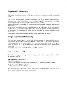
Results This section covers the results of the application of the triple exponential technique with reference to the time series data of the annual number of tourist arrivals in Nepal during the period 1971-1997.Data of the time series is extracted from different statistical year books and statistical pocket books (statistical year book of Nepal, 1987, 1989, 1991 and 1995, statistical pocket book 1982,1996 and 2000, publications o m e Central Bureau of Statistics, Thapathali, Nepal). Fig No.1 shows the time series exhibiting an approximate quadratic trend (can be verified by least square estimation).
Where ST is single smoothed statistic, S$2) is double smoothed statistic and %(3) is triple smoothed statistic and a is the exponential smoothing constant. The estimates AO(T),A1(T) and A2(T) are given by ...(7) Ao(T)=3ST- 3 ~ ~4- ( ~ ) ~ ~ ( T ) = a ( 2 ( 1 -((6-5a)~~2(5-4a)s~(~)+(4-3a)S+~)) a)~]-~ ...(8) ...(9) A2(T)= a2(1-a)-2( ~ ~ - 2 ts ~~ '~ ~ () ~ 1 ) The t period ahead forecasting equation is given by replacing the values ofAo(T), Al(T) and A2(T) in equation (3). Est. YT+t (T) 4 2 (1-a)2)-1{6(1-a12+(6-5a)at+a2t2]sT - (2(1-a)2)-1{6(1-a12+ 2(5-4a) at + 2a2t2) + (2(1-a)2)-1{2(1-a)2+ (4-3a) at + a421 s ~ (...(~10) ) In order to begin the procedure, the initial values of the Smoothed Statistics must be supplied.They are obtained by solving the equations given below 1 2 3 4 5 6 7 8 9 10 11 12 13 14 15 16 17 18 19 20 21 22 23 24 25 26 27 Year so=~ ~ ( [a~-~(l-a) 0)~ ~ ( 0 ) + ( 2 a ~ ) -(2-a) ~ ( l A2(0) - a ) ...(11) Figure 1 Line Graph of the Time Series S ~ ( ~ ) = A ~ ((a]-l(1-a) O ) - ~ A1(0)+2(2a2)-l(l-a)(3-2a) A2(0)...( 12) s ~ ( ~ ) = A ~-3{a]-'(1-a) (o) ~~(0)+3(2a~)-l(l-a)(4-3a)~~(0) ...( 13) In X axis, 1=1971,27=1997 Where Ao(O), A1(0) and A2(0) are the initial The initial values of the least square estimates of estimates of the model parameters. One way of the model parameters are found to be obtaining them are by the principle of least squares estimates of the time series. Once the initial values of b0=41816.78718, the smoothed statistic are obtained, the forecasting b1=7570.1732 and procedure is quite straightforward. In each time period, the single, double and triple smoothed statistics are computed. These smoothed statistics are then entered Changing the origin to time periodT, the estimates into the forecasting equation. The equation yields a t are period ahead forecast (Bowerman & Connell 1979). Ao(0) = 41816.78718, A1(0) = 7570.1732 and Choice of Smoothing Constant (a) A2(0) =422.92998 When an exponential smoothing procedure is used as For the chosen values of the smoothing constants a forecasting tool, the forecaster must specify a value a = 0.05,0.08 and 0.15, the initial Smoothing Statistics of the smoothing constanta. The constant determines are given in table 1. the extent to which the past observations influence the Table 1. Initial Smoothing Statistics for different forecast. In practice, it has been found that values of Values of Smoothing Constant. between 0.01 and 0.3 work quite well (Abraham & Ledolter 1983). Now the question may be if we choose between .O1 and 0.3 which value should one choose? One way of choosing involves the use of simulation. For each value of a (at an interval of say 0.03), a set of
S.L. ShresthaJNepal Journal of Science and Technology 3 (2001) 1-4 The one period ahead forecasting equations for different values of the smoothing constant are. a=0.05 Est.~+~(T)=3. 16067 ST-3.2687 S-+2)
n b l e 3. Sum of Squared Residuals (in I@) for different Values of Smoothing Constant e0.05
~-0.08
ac-0.15
DiagnosticChecking for ModelAdequacy
The one period ahead forecasts and the residuals for a=0.05 are shown in table 2. Table 3 shows the sum of squared residuals (in 109) for different values of the smoothing constant. The value of a for which the sum of squared residuals is minimum is found to be 0.05. Table 2. Estimated Values for different Values of Smoothing Constant Observed Est.1 Est.2 Est.3 Res. 1
* 1P.AF 419956.52 421213.29 427992.76 * lP.A.F= one period ahead forecast
A model that fails in diagnostic checking for model adequacy will always remain a suspect.Therefore, it is essential that model selected for forecasting should satisfy the important diagnostic checking. The following diagnostic checking are considered here. Test for Goodness of Fit The computed Coefficient of Determination (2)for smoothing constant 0.05 is equal to 0.9776, which is very high. Also if the data set of predicted values and the observed values is classified into six classes of equal intervals using Sturge's rule of classifying data, the computed value of Chi Square is only 2.7 ( I b Chi Square value for level 0.05 is 11.07) which is insignificantsuggesting that the predicted values fit to the observed time series (for a=0.05). Autocorrelation and Partial Autocorrelation Test for Residuals The assumption of no serial correlation between error variables (residuals) should not be violated while using the technique of exponential smoothing as in case of linear regression approach. The evidence of lack of significantautocorrelationsand partial autocorrelations for different lag periods is essential for verification of model adequacy test. The residual analysis shows that non of the autocorrelations and partial autocorrelations are individually statistically significant applying Bartlett approximation for significance of correlation at 95% confidence interval.This implies that the model can be accepted for forecasting ('hble 4 & 5). Table 4. Autocorrelationsfor Residuals for Smoothing Constant 0.05 Lag Correlation Error 1 2 3 4 5 6 7 8 9 10 11 12 13 14 15 16
0.118 -0.256 -0.252 0.206
0.192 0.195 0.207 0.218
0.070
0.225
-0.094 -0.334 0.020 0.087 0.05 1 -0.095 0.176 -0.179 0.075 0.075 0.004
0.226 0.228 0.245 0.245 0.246 0.247 0.248 0.253 0.257 0.258 0.259
S.L. ShresthaINepal Journal of Science and Technology 3 (2001) 1-4 Table 5. Partial Autocorrelations for Residuals for Smoothing Constant 0.05
Lag
Correlation
Error
1
0.118
0.192
2
-0.274
0.192
3
-0.198
0.192
4
0.218
0.192
5
-0.106
0.192
6
-0.059
0.192
7
-0.262
0.192
8
0.022
0.192
9
-0.084
0.192
10
-0.060
0.192
11
0.015
0.192
12
-0.267
0.192
13
-0.254
0.192
14
-0.100
0.192
15
-0.144
0.192
16
-0.115
0.192
Discussion and Conclusion The results of using the triple exponential soothing technique to the time series of the annual number of tourist arrivals in Nepal demonstrates that the method is indeed useful and suitable to such time series data exhibiting an approximate quadratic trend. This is statistically supported by performing some important diagnostic checks. Howeve~the use of this technique consumes a lot of time and computations without the support of appropriate computer programming. This is due to the simulation arising from different values of the smoothing constant. For three different values of a considered for simulation the value equal to 0.05 generates a minimum sum of squared residuals. Other values of a has been left out because of lengthy computations arising due to simulation. For the reason there can be another value of a which may generate a smaller sum of squared residuals.
References Abraham, B. & J. Ledolter 1983. Statistical Methods for Forecasting.John Wiley and Sons, Inc., USA. Bowerman, B. L. & R.T. 0' Connell1979. Eme Series and Forecasting : An Applied Approach. Wadsworth, Inc., Belmont, California, USA. Chatfield, C. 1996. The Analysis of lime Series, fifth edition. Chapman and Hall, U.K.