Application Scheduling in Mobile Cloud Computing with Load Balancing

Hindawi Publishing Corporation Journal of Applied Mathematics Volume 2013, Article ID 409539, 13 pages http://dx.doi.org/10.1155/2013/409539

Research Article Application Scheduling in Mobile Cloud Computing with Load Balancing Xianglin Wei,1 Jianhua Fan,1 Ziyi Lu,1 and Ke Ding2 1 2

Nanjing Telecommunication Technology Research Institute, Nanjing 21007, China College of Command Information Systems, PLA University of Science and Technology, Nanjing 21007, China

Correspondence should be addressed to Xianglin Wei; wei [email protected] Received 19 April 2013; Revised 15 September 2013; Accepted 27 September 2013 Academic Editor: Chih-Hao Lin Copyright © 2013 Xianglin Wei et al. This is an open access article distributed under the Creative Commons Attribution License, which permits unrestricted use, distribution, and reproduction in any medium, provided the original work is properly cited. Mobile cloud computing (MCC) enables the mobile devices to offload their applications to the cloud and thus greatly enriches the types of applications on mobile devices and enhances the quality of service of the applications. Under various circumstances, researchers have put forward several MCC architectures. However, how to reduce the response latency while efficiently utilizing the idle service capacities of the mobile devices still remains a challenge. In this paper, we firstly give a definition of MCC and divide the recently proposed architectures into four categories. Secondly, we present a Hybrid Local Mobile Cloud Model (HLMCM) by extending the Cloudlet architecture. Then, after formulating the application scheduling problems in HLMCM and bringing forward the Hybrid Ant Colony algorithm based Application Scheduling (HACAS) algorithm, we finally validate the efficiency of the HACAS algorithm by simulation experiments.

1. Introduction Recent years have witnessed the rapid development of mobile devices, such as PDAs and smartphones. The tremendous improvement of hardware and software enables them to make calls and send short messages and emails, but it also gives them the ability to sense the environment and make social contacts, health care, and mobile learning. Moreover, the inherent mobility of the mobile devices enables the users to interact with the devices, environment, and social community without time and space restriction. Thus the mobile devices are able to integrate the capabilities of communication, work, medical treatment, and mobile learning, and they become important components of people’s daily life. According to the International Data Corporation (IDC) Worldwide Quarterly Mobile Phone Tracker, it is estimated that 982 million smartphones will be shipped worldwide in 2015 [1]. However, mobile devices also have some inherent defects, such as their limited battery energy, low CPU speed, insufficient storage space, and inadequate sensing capacities [2]. These limitations have brought for mobile applications many challenges in mobility management, quality of service (QoS) insurance, energy management, and security issues.

On the other hand, the lack of resources also motivates the researchers in mobile computing area to search for the infrastructure which can provide the needed resources for the mobile devices [3]. Consequently, cloud computing was introduced to fulfill this gap since it can theoretically provide nearly inexhaustible resources for mobile computing. The combination of cloud computing and mobile computing has stimulated the emergence of mobile cloud computing (MCC). MCC brings rich resources of the cloud computing for mobile devices and applications, as well as inheriting the cloud’s advantages, such as low cost, high scalability, and robustness. Therefore, it greatly improves the potential of mobile computing. In MCC environment, mobile devices can offload full or part of their mobile applications to the data centers of the cloud in order to relieve their own burden in CPU load and energy consumption. This enables them to support more sophisticated and richer applications and services, such as mobile game [4], mobile locating [5], voice, key words and picture searching [6–8], and mobile sensing [9]. In order to support these applications, researchers have proposed various architectures for MCC, such as MobiCloud, MAUI, CloneCloud, Cloudlet, and Hyrax. These proposals

2 attempt to utilize the cloud infrastructure as well as the mobile devices’ idle CPUs or sensing capacities to achieve high QoS. However, offloading to remote cloud infrastructure will introduce long response latency. Hence, to reduce the response latency, the offloaded applications should be handled by local cloud infrastructure, which usually has fewer resources than those of the remote ones. Therefore, how to efficiently schedule the limited resources while fulfilling the requirements of a large number of offloaded applications is a critical problem for MCC to address. In this paper, we first give the definition of MCC and divide the recently proposed architectures into four categories. Secondly, Hybrid Local Mobile Cloud Model (HLMCM) is put forward after combining the advantages of current proposals, such as Cloudlet and Hyrax. Thirdly, we formulate the application scheduling problems in HLMCM and bring forward the Hybrid Ant Colony algorithm based Application Scheduling (HACAS) algorithm. Finally, the effectiveness of HACAS algorithm is validated by simulation experiments. The rest of the paper is organized as follows. Section 2 summarizes related work. Section 3 gives the definition of MCC and introduces the HLMCM. Section 4 formulates the application scheduling problem and proposes HACAS algorithm. Simulation experiments and results are shown in Section 5. Finally, we conclude our main work and present further research directions in Section 6.

2. Related Work Application scheduling in cloud infrastructure has attracted much attention in recent years. In fact, the application scheduling and load balancing in MCC are burgeoning areas. Liu et al. have established a macroscopic scheduling model with cognition and decision components for the cloud computing, which considers both the requirements of different jobs and the circumstances of computing infrastructure. They have also put forward a job scheduling algorithm based on Multiobjective Genetic Algorithm (MO-GA), taking into account the energy consumption and the profits of the service providers [10]. In order to reduce the operator cost and to increase the reliability of the cloud service provider, Feller et al. have modeled the workload placement problem as an instance of the multidimensional bin-packing (MDBP) problem and have designed a novel, nature-inspired algorithm based on the Ant Colony Optimization (ACO) metaheuristics to compute the placement dynamically, according to the current load [11]. Goudarzi and Pedram have considered a multitier cloud computing environment, in which the clients have Service Level Agreements (SLAs) and the total profit in the system depends on how the system can meet these SLAs. They have proposed an algorithm based on forcedirected search to allocate the resources, such as processing, memory requirement, and communication resources [12]. In the shared data center environment, Nagendram et al. have depicted the resource scheduling problem to a bounded multidimensional knapsack problem, taking into account the requirement dependency among multidimensional resources

Journal of Applied Mathematics including memory, storage, CPU, and network bandwidth. Then, they have presented a Multidimensional resource integrated scheduling (MRIS), an inquisitive algorithm to obtain the approximate optimal solution [13]. To schedule the tasks and achieve load balance, Tayal has put forward an optimized algorithm based on the Fuzzy-GA optimization which makes a scheduling decision by evaluating the entire group of tasks in the job queue [14]. In the private cloud environment constructed for e-learning, Morariu et al. have presented a workload scheduling algorithm based on genetic algorithm [15]. For the load balancing problem of the VM scheduling in the cloud computing, Gu et al. have proposed a scheduling strategy on load balancing of VM resources based on genetic algorithm [16]. Yamauchi et al. proposed a distributed parallel scheduling methodology for MCC and developed a simulator to analyze the bottleneck of MCC [17]. Ant Colony Optimization (ACO) has also been used to balance the load in cloud environment. In [18], Mishra et al. have proposed a method to utilize the ACO for load balancing in cloud environment. The routing packets in this environment are treated as the ants in the network. Moreover, they replaced the routing tables in the network nodes by tables of probabilities. These tables are also called “pheromone tables” since the pheromone strengths used in ACO are represented by these probabilities. Every node has a pheromone table for every possible destination in the network, and each table has an entry for every neighbor. The entries in the tables are the probabilities which influence the ants’ selection of the next node on the way to their destination node. Consequently, at each node, the ant should choose the next node toward its final destination node according to the probabilities. After arriving at a node, the ants update the probabilities of that node’s pheromone table entries corresponding to their source node; that is, ants lay the kind of pheromone associated with the node they were launched from. They alter the table to increase the probability pointing to their previous node. Besides, in order to distribute the load among many paths from the source node to the destination node, the ants from one colony will consult the routing tables of other colonies so as to avoid routing packets to those paths that are highly preferred by the other groups. Through this method, the loads are separated among many possible paths in the network. Zhu et al. considered the task scheduling in cloud environment from the perspectives of QoS fulfillment and shortest path [19]. Nishant et al. have proposed an algorithm for load distribution of workloads among nodes of a cloud by the use of ACO. Moreover, they have presented another load balancing algorithm which ensures that there is no conflict of interests based on relocating the tasks among nodes [20]. In these works, they do not take each task’s profit into consideration and cannot maximize the profit of the system, which is an import target of the scheduling algorithm for the commercial mobile cloud environment. In grid computing, an ACO algorithm is proposed by Suryadevera et al. for load balancing which will determine the best resource to be allocated to the jobs, based on resource capacity, and at the same time balance the load of entire resources on grid. The main objective of this algorithm is to achieve high throughput and thus increases the performance in grid environment

Journal of Applied Mathematics [21]. A review on the load balancing studies for the cloud environment is presented in [22]. Different from the scheduling algorithm in cloud environment, the scheduling algorithms for MCC should take the energy consumption into consideration. To make the system last longer, the scheduling algorithms should balance the load of the mobile devices to avoid some heavy-loaded nodes leaving the system too early. Therefore, these scheduling algorithms for cloud computing cannot be applied to the MCC environment directly. In order to bridge this gap, we propose an architecture for MCC and then present a scheduling algorithm for MCC which can maximize the profit and balance the load of the mobile devices.

3. Definition and Architecture 3.1. The Definition of MCC and Current Proposed Architectures. The Mobile Cloud Computing Forum defines MCC as follows [23]: “Mobile cloud computing, at its simplest, refers to an infrastructure where both the data storage and the data processing happen outside of the mobile device. Mobile cloud applications move the computing power and data storage away from mobile phones and into the cloud, bringing applications and mobile computing to not just smartphone users but a much broader range of mobile subscribers.” Aepona describes MCC as a new paradigm for mobile applications whereby the data processing and storage are moved from the mobile device to powerful and centralized computing platforms located in clouds [24]. These centralized applications are then accessed over the wireless connection based on a thin native client or web browser on the mobile devices. In [25, 26], MCC is described as a combination of mobile web and cloud computing, which is the most popular tool for mobile users to access applications and services on the Internet. Dinh et al. defined MCC as an entity that provides mobile users with the data processing and storage services in clouds [27]. These definitions are mostly descriptive. This paper gives the following definition: MCC is a mobile applicationoriented computing paradigm in mobile and dynamic environment, which makes use of the resources provided by clouds, mobile devices, and network facilities to fulfill users’ requirements on QoS, quality of experience (QoE), security and privacy, with some particular cost, energy, and programming model and context information. In order to efficiently utilize the available resources, researchers have brought forward several MCC architectures. In this paper, we divide them into four categories. In the proposals of the first category, mobile devices first offload applications to the remote large data centers of the clouds, from which the results will be returned; the typical proposals include MAUI [28] and CloneCloud [29]. In the second category, Satyanarayanan et al. introduced the Cloudlet entity to the system, which is a local service infrastructure logically implemented at the access point of mobile devices, and the mobile devices only have to offload applications to the Cloudlet rather than remote data centers [27, 30]. It should be noted that Cloudlet can reduce the server response latency

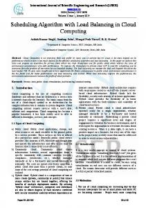
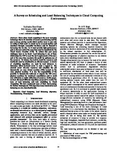
3 since the offloading happens locally most of the time. In the proposals of the third category, mobile devices collaborate with each other to run applications without the need to rely on any cloud infrastructure. This sounds like the mobile Peerto-Peer system and mobile grid computing, but different from these computing paradigms, the typical schemes (such as Hyrax [31] Misco [32], and the virtual cloud [33]) of this category adopt the unique characteristics of MCC such as fault tolerant and application partition. The typical schemes of the fourth category move the cloud infrastructure close to the users to improve the timeliness of the service, such as MobiCloud [34–36]. Figure 1 illustrates the traditional architecture which uses remote cloud infrastructure via the backbone network. As shown in Figure 1, the latency of this architecture consists of the time spent on the access network, the backbone network, and the time spent inside the cloud infrastructure. In the Cloudlet architecture, as shown in Figure 2, most of the time, the application will not deliver to the remote cloud infrastructure, and thus the latency is composed of the one-hop time spent on the access network, which is much lower than those using architecture of Figure 1 [30, 37]. Under some special conditions, Cloudlet cannot handle the offloaded applications locally, and it needs the remote cloud infrastructure’s help for processing them. The latency under these conditions approximates the traditional architecture which directly uses the remote cloud infrastructure. 3.2. Hybrid Local Mobile Cloud Model. In order to provide high QoS for mobile applications, the MCC architecture should have low response latency. Moreover, the mobile devices’ participation for providing their idle computing and sensing capabilities is also very critical for the promotion of the users’ QoE (quality of experience). This is due to the fact that one single mobile device’s sensing result can be easily influenced by its local environment and hence is errorprone, while aggregating a few mobile devices’ sensing results about the area can provide more correct context information. Therefore, we have modified the Cloudlet architecture to make the mobile devices contribute their computing and sensing capabilities like they do in Hyrax [31] and Misco models [32]. This new mobile cloud computing model is called the Hybrid Local Mobile Cloud Model (HLMCM) and is illustrated in Figure 3. From Figure 3, we can see that HLMCM consists of a Cloudlet and a set of mobile devices. The mobile devices are connected to the Cloudlet via wireless links, such as WiFi and WiMAX. Similar to the original Cloudlet architecture, the Cloudlet in HLMCM is logically attached to the access point of the mobile devices to achieve low response latency, and the mobile devices can offload their mobile applications to the Cloudlet. However, different from Satyanarayanan’s scheme [30], in HLMCM, the mobile devices collaborate with the Cloudlet to provide service. This designation is based on the following considerations. (1) Mobile devices’ computing, storage, and sensing capabilities are increasingly becoming powerful. However, the utilization ratio of these resources is low

4

Journal of Applied Mathematics

Cloud infrastructure

···

Backbone network

Mobile devices

Figure 1: The architecture that uses the remote cloud infrastructure.

Cloud infrastructure

Backbone network

···

Cloudlet

Mobile devices

Figure 2: The Cloudlet architecture.

···

Cloudlet

(1) Client (4) (1) Client (4)

Mobile devices

Figure 3: The architecture of the hybrid local mobile cloud model.

(1)

Client

(4)

Cloudlet

(2) (3)

(2) (2) (3) (3)

Mobile devices

Figure 4: The general working process of HLMCM.

at most times, which means that the mobile devices usually have idle resources for sharing.

(3) The involvement of the mobile devices can help improve the QoS provided by HLMCM, especially the sensing capabilities.

(2) The Cloudlet usually only contains a few servers and is much less powerful than the data center of the typical large-scale cloud. Therefore, the mobile devices’ participation can promote the scalability of HLMCM.

The general working process of HLMCM is shown in Figure 4, and it mainly contains the following four steps. (1) The clients offload part or full of their applications to the Cloudlet. Note that the clients are mobile devices


5

as well, and they can provide service for other devices’ mobile applications. (2) The Cloudlet executes the application scheduling algorithm to offload the applications to a few mobile devices that are willing to provide resources. (3) The mobile devices handle the applications received and send their results to the Cloudlet. (4) The Cloudlet sends the results of the applications from the mobile devices to the clients. Note that there may be a large number of mobile devices requesting for offloading applications to the HLMCM whose sensibility, computing, and storage capabilities are usually much less than those of the large cloud infrastructure. Therefore, efficient application scheduling algorithm is critical for HLMCM to provide high QoS. Moreover, the application scheduling algorithm should consider the profits of the HLMCM as well as balancing the load of the mobile devices to make the whole system last longer.

4. Model and Algorithm 4.1. Model and Problem Statement. In HLMCM environment, the scheduling algorithm is in charge of allocating the offloaded applications from the mobile devices to the service providers, including the Cloudlet and 𝑚−1 mobile devices in the system. For ease of description, the service provider will be referred to as provider in the following analysis. Assume the dimension of the resources is 𝑑 and each provider’s resources can be expressed as a vector 𝑐𝑖⃗ = (𝑐𝑖1 , . . . , 𝑐𝑖𝑑 ), in which 𝑐𝑖𝑘 is the 𝑘th dimensional resource that the provider 𝑖 has. Assume that the set of applications that arrives at some particular time slot is 𝐼 = {1, 2, . . . , 𝑛}, and the value of the application 𝑗 is 𝑝𝑗 , 𝑗 = 1, 2, . . . , 𝑛. The resources consumed by application 𝑗 when executed on provider 𝑖 are a vector 𝑟𝑖𝑗⃗ = (𝑟𝑖𝑗1 , . . . 𝑟𝑖𝑗𝑑 ), 𝑖 = 1, 2, . . . , 𝑚. Assume that each application can only be executed on one provider and cannot be further partitioned. Once an application is executed successfully on some provider, HLMCM will receive the value of this application as its profit. Here, the scheduling target is to maximize the total profits of HLMCM with the constraint of resource capacity of each service provider. Therefore, the scheduling problem can be formulated as follows. Maximize

𝑛

𝑚

𝑗=1

𝑖=1

∑ 𝑝𝑗 ∑𝑥𝑖𝑗 𝑛

subject to

∑𝑟𝑖𝑗⃗ 𝑥𝑖𝑗 ≤ 𝑐𝑖⃗ ,

𝑖 = 1, 2, . . . , 𝑚

𝑗=1 𝑚

∑𝑥𝑖𝑗 ≤ 1,

(1) 𝑗 = 1, 2, . . . , 𝑛

𝑖=1

𝑥𝑖𝑗 ∈ {0, 1} ,

𝑗 = 1, 2, . . . , 𝑛.

From (1), we can see that this can be seen as a multidimensional 0-1 knapsack problem and is NP-hard.

Besides, in order to make HLMCM last longer, the applications should be uniformly executed on the mobile devices. This will make the devices consume their energy evenly to avoid the phenomenon that some mobile devices with heavy load consume their energy too early and have to leave the system. For some particular provider 𝑖, the load of its 𝑘th dimensional resource is defined as. 𝐿 𝑖𝑘 =

∑𝑛𝑗=1 𝑟𝑖𝑗𝑘 𝑥𝑖𝑗 𝑐𝑖𝑘

.

(2)

𝑖󸀠 s load 𝐿 𝑖 is defined as the mean value of all its 𝑑-dimensional resources’ loads; that is, 𝐿𝑖 =

∑𝑑𝑘=1 𝐿 𝑖𝑘 . 𝑑

(3)

4.2. HACAS Algorithm. In order to solve this problem, this paper proposes a scheduling algorithm based on the hybrid ant colony algorithm which has been widely used to solve complex combinatorial optimization problems [38]. The following part of this section presents HACAS algorithm, which contains the pheromone value and its update model, local heuristic value, application scheduling probability, tabu list and the bulletin board, and provider selection scheme. 4.2.1. Pheromone Value and Its Update Model. The application scheduling problem in this paper belongs to the subset problem [39]; that is, given a set 𝑆 which contains 𝑛 applications for scheduling and the evaluation function 𝑓( ), the target is to select the best subset of 𝑆 to maximize or minimize 𝑓( ). There may be more than one evaluation functions while this section focuses on the case where there is only one evaluation function. In this situation, the order of the selected applications is not important, and the pheromone value is placed on the application rather than the connection among the applications, which means that applications with a higher pheromone value can better satisfy the requirements of the evaluation function. When the specific condition is met, such as a partial solution with some particular length is obtained, the pheromone value needs to be updated. The update process includes two parts. Firstly, the pheromone value of each application is reduced by a certain percentage to emulate the real-life behavior of evaporation of pheromone count over time; Secondly, the pheromone value increment laid by the new partial solutions of the ants will be added. Assume that the pheromone value on application 𝑖 at time 𝑡 is 𝜏𝑖 (𝑡); then at the next update time 𝑡󸀠 , the value is updated to 𝜏𝑖 (𝑡󸀠 ): 𝜏𝑖 (𝑡󸀠 ) = (1 − 𝜌) 𝜏𝑖 (𝑡) + Δ𝜏𝑖 (𝑡, 𝑡󸀠 ) ,

(4)

where 0 < 𝜌 ≤ 1 is a coefficient which represents pheromone evaporation, Δ𝜏𝑖 (𝑡, 𝑡󸀠 ) is the pheromone value increment obtained from all the ants’ partial solutions; that is, 𝑞

𝑗

Δ𝜏𝑖 (𝑡, 𝑡󸀠 ) = ∑ Δ𝜏𝑖 (𝑡, 𝑡󸀠 ) , 𝑗=1

(5)

6

Journal of Applied Mathematics 𝑗

where 𝑞 is the number of the ants and Δ𝜏𝑖 (𝑡, 𝑡󸀠 ) is the pheromone value laid on application 𝑖 by ant 𝑗’s partial solution at time 𝑡󸀠 and is defined as 𝑗

Δ𝜏𝑖 (𝑡, 𝑡󸀠 ) 𝐺 (𝑓 (𝑆̃𝑗 (𝑡󸀠 ))) , ={ 0,

if 𝑗th ant incoporates application 𝑖 otherwise, (6)

where 𝑆̃𝑗 (𝑡󸀠 ) is the partial solution of ant 𝑗 at time 𝑡󸀠 and 𝑓(𝑆̃𝑗 (𝑡󸀠 )) is the value of the evaluation function of this solution. To maximize the profit, the evaluation is defined as 𝑓 (𝑆̃𝑗 (𝑡󸀠 )) =

∑ 𝑝𝑘 ; 𝑘∈𝑆̃𝑗 (𝑡󸀠 )

(7)

that is, the total value of the applications belongs to 𝑆̃𝑗 (𝑡󸀠 ). The function 𝐺 in (4) depends on the problem; in this paper, it is defined as 𝐺(𝑓(𝑆̃𝑗 (𝑡󸀠 ))) = 𝑄𝑓(𝑆̃𝑗 (𝑡󸀠 )), in which 𝑄 is a parameter of the method. 4.2.2. Local Heuristic Value. The positive feedback of the ant colony algorithm is usually combined with some local heuristic schemes to accelerate the search process. In HLMCM, the local heuristic scheme needs to consider the profits of the applications as well as the resources they consume. Let 𝜇𝑘⃗ (𝑗, 𝑡) = ∑𝑙∈𝑆̃𝑗 (𝑡) 𝑟𝑘𝑙⃗ be the resources consumed on provider 𝑘 by the partial solution 𝑆̃𝑗 (𝑡) constructed by ant 𝑗. Then, the remaining resources on provider 𝑘 are 𝛾𝑘⃗ (𝑗, 𝑡) = 𝑐𝑘⃗ − 𝜇𝑘⃗ (𝑗, 𝑡) = (𝛾𝑘1 (𝑗, 𝑡), . . . , 𝛾𝑘𝑑 (𝑗, 𝑡)), in which 𝛾𝑘𝑖 (𝑗, 𝑡) is the remaining amount of the 𝑖th dimensional resource. The tightness of application ℎ on provider 𝑘 on the 𝑖th dimensional resource is defined as 󵄨 󵄨󵄨 𝑟𝑖 󵄨󵄨 𝑘ℎ 󵄨󵄨󵄨 󵄨 󵄨󵄨 𝑖 (8) 󵄨󵄨 𝛾 (𝑗, 𝑡) 󵄨󵄨󵄨 󵄨 󵄨 𝑘 𝑖 that is the ratio between 𝑟𝑘ℎ , the amount of provider 𝑘’s resource consumed by application ℎ, and 𝛾𝑘𝑖 (𝑗, 𝑡). Moreover, the tightness of application ℎ on provider 𝑘 is defined as 󵄨󵄨 𝑑 󵄨󵄨 󵄨󵄨 𝑟1 󵄨󵄨 󵄨󵄨 𝑟 󵄨󵄨 󵄨 󵄨 (9) 𝛿𝑘ℎ (𝑗, 𝑡) = 󵄨󵄨󵄨󵄨 1 𝑘ℎ 󵄨󵄨󵄨󵄨 + ⋅ ⋅ ⋅ + 󵄨󵄨󵄨 𝑑 𝑘ℎ 󵄨󵄨󵄨 . 󵄨󵄨 𝛾 (𝑗, 𝑡) 󵄨󵄨 󵄨󵄨 𝛾𝑘 (𝑗, 𝑡) 󵄨󵄨 󵄨 𝑘 󵄨 In (9), the tightness of the 𝑑-dimensional resources is converted into a single value which comprehensively considers all dimensions of the resources. The average tightness on all providers in case of application ℎ being chosen to be included in 𝑆̃𝑗 (𝑡) is

∑𝑚 𝑘=1 𝛿𝑘ℎ (𝑗, 𝑡) (10) . 𝑚 In order to consider the application ℎ’s profit as well as its resource requirement, the local heuristic value 𝜂ℎ (𝑆̃𝑗 (𝑡)) is defined as 𝑝ℎ . 𝜂ℎ (𝑆̃𝑗 (𝑡)) = (11) 𝛿ℎ (𝑗, 𝑡) 𝛿ℎ (𝑗, 𝑡) =

4.2.3. Application Scheduling Probability. After obtaining the pheromone value and local heuristic value on each application, the probability that ℎ has to be selected as the next scheduling application of 𝑆̃𝑗 (𝑡) is 𝑗

𝑃ℎ (t) 𝛽 [𝜏ℎ (𝑡)]𝛼 [𝜂ℎ (𝑆̃𝑗 (𝑡))] { { { , if ℎ ∈ allowed𝑗 (𝑡) { 𝛼 = {∑ ̃𝑗 (𝑡))]𝛽 [𝜏 [𝜂 ( 𝑆 (𝑡)] 𝑘 𝑘 { 𝑘∈allowed𝑗 (𝑡) { { 0, otherwise, { (12)

where allowed𝑗 (𝑡) ⊆ 𝑆 − 𝑆̃𝑗 (𝑡), is the set of the remaining schedulable applications. From (12), we can see that the more pheromone value and local heuristic value an application has, the higher the probability will be scheduled. 4.2.4. Tabu List and the Bulletin Board. A data structure, called a tabu list, is associated to each ant in order to avoid that ant from scheduling an application more than once. This list tabu𝑗 (𝑡) maintains a set of scheduled applications up to time 𝑡 by ant 𝑗. Let the applications that can be executed on at least one of the providers be 𝐹; then we have allowed𝑗 (𝑡) = 𝐹 ∩ {ℎ | ℎ ∉ tabu𝑗 (𝑡)}. In addition, we set a bulletin board to record the best solution up to time 𝑡, with which each ant can compare its own solution. If its solution is better than the best one, it will update the best one with its solution. 4.2.5. Provider Selection Scheme. After deciding the scheduled application, there is usually more than one provider who have sufficient resources to execute the application. Note that traditional hybrid algorithm only focuses on the application scheduling probability. In order to balance the load of the providers, we take the provider selection scheme into consideration in this section. For some particular feasible provider 𝑖, the load of its 𝑘th dimensional resource is 𝐿 𝑖𝑘 as defined in (2). After adding application ℎ, the expected load of its 𝑘th dimensional resource is 𝐿󸀠𝑖𝑘 = 𝐿 𝑖𝑘 +

𝑘 𝑟𝑖ℎ

𝑐𝑖𝑘

.

(13)

The expected load of provider 𝑖 is defined as 𝐿󸀠𝑖 =

∑𝑑𝑘=1 𝐿󸀠𝑖𝑘 . 𝑑

(14)

This means that if is ℎ executed on provider 𝑖, 𝑖’s expected load will be 𝐿󸀠𝑖 . In order to balance the load of all the providers, the provider with the lowest expected load will be selected to execute application ℎ. 4.2.6. Algorithm. The HACAS algorithm is illustrated in Algorithm 1. The parameters needed to be settled include 𝐶,


7

(1) Initialize 𝑟𝑖𝑗⃗ , 𝑐𝑖⃗ , 𝑝𝑗 , 1 ≤ 𝑖 ≤ 𝑚, 1 ≤ 𝑗 ≤ 𝑛, 𝑞 = 𝑛, number of cycles 𝐶, 𝜏𝑗 (0) = 1/𝑞, 1 ≤ 𝑗 ≤ 𝑞, tabu list = [], best solution = 0, application provider, 𝛼 = 𝛽 = 1, 𝜌 = 0.3, 𝑄 = 1 (2) for (𝑡 = 1: 𝑡 best solution (19) best solution = 𝑓(𝑆̃𝑗 (𝑡)) (20) Save ant j’s solution in application provider (21) end if (22) end for (23) Calculate the incremental pheromone on each application according to (5) (24) Clear the tabu list for each ant (25) end for (26) print best solution (27) print application provider Algorithm 1: The HACAS algorithm.

𝛼, 𝛽, 𝜌, 𝑞, 𝑄, 𝑟𝑖𝑗⃗ , 𝑐𝑖⃗ , and 𝑝𝑗 . The initial pheromone trail value on each application is set to be 1/𝑞. Step 1 initiates the parameters. Step 4 introduces a variable random first to enable each ant to randomly select its first scheduling application. Steps 5 to 16 present the solutionsearching process of an ant. Firstly, Steps 6 to 11 select the next scheduled application, that is, randomly selecting the first one and then scheduling other applications according to the probabilities calculated in (12). Secondly, Step 12 calculates the expected loads of all feasible providers according to (14), Step 13 ranks the feasible providers according to their expected loads in an increasing order, Step 14 selects the provider with the lowest expected load for ℎ, and finally, Step 15 adds the newly scheduled application to the partial solution as well as the tabu list. At the end of Step 16, each ant has found its solution 𝑆̃𝑗 (𝑡); Step 17 calculates 𝑓(𝑆̃𝑗 (𝑡)). If 𝑓(𝑆̃𝑗 (𝑡)) is larger than the best solution in the bulletin board, then Step 19 will assign 𝑓(𝑆̃𝑗 (𝑡)) to best solution and save the scheduling results into application provider. After Step 22, all the ants have finished searching for the solutions, and one cycle is finished. Step 23 calculates the pheromone value increment according to (5). Step 24 clears the tabu lists of the ants. Steps 26 to 27 print the best solution found at the 𝐶th cycle and the scheduling results.

5. Simulation, Results, and Discussion 5.1. Experimental Settings 5.1.1. Experimental Environment. To evaluate the performance of the algorithms proposed in this paper, we have conducted many simulation experiments, whose parameters are listed in Table 1. In this simulation, the dimension of the resources is 2. Both the first and the second dimensional resources possessed by each provider obey uniform distribution in the interval [𝑎1 , 𝑎2 ]. There are 𝑚 providers and 𝑛 applications in the system. At time 𝑡, these applications arrive simultaneously. The applications’ resource consumption of the first and the second dimensional resources on some provider obeys uniform distribution in the intervals [𝑎3 , 𝑎4 ] and [𝑎5 , 𝑎6 ], respectively. Moreover, the applications’ profits obey uniform distribution in the interval [𝑎7 , 𝑎8 ]. The number of cycles (i.e., 𝐶) is set to be 10. The default parameters are listed in Table 1. Based on these parameters, a series of simulation experiments has been conducted. The experiments contain 10 cycles. In each cycle, each ant searches for its own scheduling result based on the method presented in the scheduling algorithm in the above section. At the end of each cycle,

8

Journal of Applied Mathematics 𝑗

Table 1: Simulation parameters. Parameter 𝑛 𝑎1 𝑎2 𝑎3 𝑎4 𝑎5 𝐶 𝛽 𝑄 𝑚 𝑎6 𝑎7 𝑎8 𝛼 𝜌 𝜃 𝜆

Default Value 100 31 100 10 30 10 10 1 1 20 30 5 30 1 0.3 1 1

the pheromone value on the applications will be updated and the bulletin board is used to record the best scheduling result. 5.1.2. Comparison Benchmark and Metrics. We evaluate HACAS algorithm from two different angles. Firstly, in order to validate the effectiveness of HACAS algorithm, we compare it with the First-Come-First-Served (FCFS) algorithm. In FCFS, the applications are scheduled according to their arrival order, and the providers are selected randomly from those who can execute the application. The profit of the scheduling algorithm, which is defined as the total profits of all the applications scheduled by the algorithm, is chosen as the metrics to compare them. Secondly, in order to evaluate the provider selection scheme of HACAS algorithm, a scheduling algorithm with random provider selection is adopted as the comparison benchmark, in which steps 12–14 in Algorithm 1 are replaced with the following step. (12) Randomly select the service provider for ℎ from those feasible providers. The scheduling algorithm with this modification is called the Hybrid Ant Colony algorithm based Application Scheduling with Random Provider Selection (HACASRPS) algorithm. For the solution of ant 𝑗 at the 𝑘th cycle, let provider 𝑖’s 𝑗𝑘 𝑗 load be 𝐿 𝑖 . The mean value (𝜇𝑘 ) and the standard deviation 𝑗 (𝜎𝑘 ) of all the 𝑚 providers’ loads at the 𝑘th cycle of ant 𝑗’s solution are defined as 𝑗

𝜇𝑘 = 𝑗 𝜎𝑘

𝑗𝑘

∑𝑚 𝑖=1 𝐿 𝑖 , 𝑚

1 𝑚 𝑗𝑘 𝑗 2 = √ ∑(𝐿 𝑖 − 𝜇𝑘 ) . 𝑚 𝑖=1

(15)

𝜎𝑘 reflects the deviation of all the providers’ loads of ant 𝑗’s solution at the 𝑘th cycle. Then, at the end of the 𝑘th cycle, the mean value of the standard deviation of all the providers’ loads of all the 𝑞 ants’ solution is defined as 𝑗

𝑞

𝜇𝜎𝑘 =

∑𝑗=1 𝜎𝑘 𝑞

.

(16)

In order to simplify the expression, 𝜇𝜎𝑘 will be referred to as the load variation of the scheduling algorithm at the 𝑘th cycle. Then, the average load variation of the scheduling algorithm of all the simulation cycles can be defined as 𝜇𝜎 =

∑𝐶𝑘=1 𝜇𝜎𝑘 . 𝐶

(17)

We define the average load of a scheduling algorithm in 𝑘th cycle by 𝑗

𝑞

𝜇𝜇𝑘

=

∑𝑗=1 𝜇𝑘 𝑞

.

(18)

Then the average load of a scheduling algorithm is defined by 𝜇𝜇 =

∑𝐶𝑘=1 𝜇𝜇𝑘 𝐶

.

(19)

𝑗

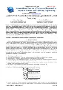
𝜎𝑘 , 𝜇𝜇 , and 𝜇𝜎𝑘 are selected as the metrics to evaluate the effectiveness of the provider selection scheme of the HACAS algorithm. 5.2. Experimental Results 5.2.1. The Profits. With the parameters in Table 1, the profit of FCFS algorithm is 1324. The profits of HACASRPS and HACAS algorithms are shown in Figure 5. From Figure 5, we can see that as cycle increases, the profits of both HACASRPS and HACAS algorithms increase. This is due to the fact that as cycle increases, both the HACASRPS and HACAS algorithms will find more profitable scheduling results which will bring more profits. At the end of the 10th cycle, the profits of HACASRPS and HACAS algorithms are 1747 and 1794, respectively, which are more than 30% higher than that of FCFS algorithm. This phenomenon can be attributed to the local heuristic value adopted by both algorithms, which enables them to schedule those applications which consume less resources while bringing more profits with preference. 5.2.2. Load Balancing. Balancing the load of all the providers to make the system last longer is an important target of HACAS algorithm’s provider selection scheme. This section investigates the effectiveness of this selection scheme and compares it with random provider selection method adopted in HACASRPS algorithm. With the parameters in Table 1, the average loads of HACAS and HACASRPS algorithms are 0.800 and 0.779,


9

1800

0.13 0.125

1750

0.12 𝜇𝜎k

Profit

1700

1650

0.11

1600

1550

0.115

0.105 0.1 1

2

3

4

5

6

7

8

9

10

1

2

3

6

7

8

9

10

HACASRPS HACAS

HACASRPS HACAS

Figure 5: The profits of HACASRPS and HACAS algorithms. The horizontal axis represents the simulation cycle; the longitudinal axis represents the profit of the algorithm.

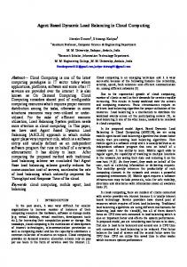
Figure 7: The load variations of HACAS and HACASRPS algorithms in different simulation cycles; 𝑘 is the simulation cycle, and 𝜇𝜎𝑘 is the load variation of the algorithm in the 𝑘th cycle.

in different simulation cycles, and the results are shown in Figure 7. From Figure 7, we can see that the load variations of these two algorithms maintain stable as simulation cycle increases. Moreover, the load variation of HACAS algorithm is much lower than that of HACASRPS algorithm. In some particular cycle, HACAS algorithm’s load variation is about 13% lower than that of the HACASRPS algorithm. This is because the provider selection scheme adopted in HACAS algorithm takes the providers’ load into account when choosing the provider for the scheduled applications. This means that the provider selection scheme in HACAS algorithm can effectively balance the load of the providers more effectively.

0.83 0.82 0.81 𝜇𝜇k

5 k

Cycle

0.8 0.79 0.78 0.77

4

1

2

3

4

5

6

7

8

9

10

k

HACASRPS HACAS

Figure 6: The average load of HACAS and HACASRPS algorithms in different simulation cycles; 𝑘 is the simulation cycle, and 𝜇𝜇𝑘 is the average load of the algorithm in the 𝑘th cycle.

respectively. The former is slightly higher than the latter, which is due to the fact that HACAS schedules more applications than HACASRPS algorithm as shown in Figure 5. The average load of HACAS and HACASRPS algorithms in different simulation cycles (as defined in (18)) are shown in Figure 6. From Figure 6, we can see that the average load of both algorithms stays stable as cycle increases. Figure 6 tells us that the average loads of HACAS and HACASRPS algorithms are 0.8 and 0.78, respectively. We further investigate the load variations of both algorithms

5.2.3. Parameters’ Influence. In the above experiments, the number of the applications for scheduling is large and the load of the providers is high. This section shows the results when the number of the applications for scheduling is relatively small. Concretely speaking, we set 𝑚 = 20 with 𝑛 = 30 in this experiment. Firstly, we investigate the load of all the providers of the 10th ant’s solution at the 5th cycle, and the results are shown in Figure 8. From Figure 8, we can see that the load of the providers in HACASRPS algorithm fluctuates in a much wider range than that of HACAS algorithm. In HACASRPS algorithm, the load of the 7th provider is almost 0.8, while the loads of the 16th and the 18th provider are 0. In contrast, the load of the providers in HACAS algorithm is mostly between 0.3 and 0.6. The notable differences of the resource consumption among different applications (from 10 to 30) have led to the differences among the loads of the providers. Then we show the standard deviation of all the providers’ loads of the ant’s solution in the 5th cycle in Figure 10. Note that there are 30 ants in the algorithm since 𝑞 = 𝑛.

10

Journal of Applied Mathematics 0.28

0.8

0.26

0.7

0.22

0.5

0.2 𝜇𝜎k

The load of the provider

0.24 0.6

0.4

0.18 0.16

0.3

0.14

0.2

0.12

0.1

0.1

0

0.08 0

5

10 Provider

15

2

3

4

5

6

7

8

9

10

k

HACASRPS HACAS

HACASRPS HACAS

Figure 8: The load of all the providers of the 10th ant’s solution at the 5th cycle.

Figure 10: The load variations of HACAS and HACASRPS algorithms in different simulation cycles; 𝑘 is the simulation cycle, and 𝜇𝜎𝑘 is the load variation of the algorithm in the 𝑘th cycle.

selection scheme of the HACAS algorithm becomes more prominent when the load of the system is low.

0.4 The standard deviation of all the providers’ load of the ant’s solution

1

20

0.35

5.3. Discussion and Application Scenario

0.3 0.25 0.2 0.15 0.1 0.05

0

5

10

15 Ant

20

25

30

HACASRPS HACAS

Figure 9: The standard deviation of all the providers’ loads of the ant’s solution in the 5th cycle.

Figure 9 reveals that the standard deviations of all the providers’ loads of the ant’s solution of HACAS algorithm are much lower than those of the HACASRPS algorithm. Similar to Figure 7, Figure 10 further reveals the load variations of HACAS and HACASRPS algorithms in different simulation cycles when 𝑛 = 30, from which we can derive similar observations with those drawn from Figure 7. Moreover, in some particular cycle in Figure 10, HACAS algorithm’s load variation is about 60% lower than that of the HACASRPS algorithm. Therefore, after combining Figures 7 and 10, we know that the effectiveness of the provider

5.3.1. Discussion. As shown in Section 5.2, the performance of HACAS algorithm is better than that of FCFS and HACASRPS algorithms. This phenomenon can be attributed to HACAS algorithm’s pheromone value and its update model, application scheduling model, and provider selection scheme. Concretely speaking, pheromone value and its update model make HACAS learn from its historical decision to raise the profit of the system. Moreover, application scheduling model takes the pheromone value as well as application’s resource consumption into consideration and can help HACAS algorithm choose those applications with the highest profit and the lowest resource consumption. Last but not the least, the provider selection scheme can balance the load of the mobile devices, which is very important to make the system last longer. In addition, the following section shows the reason why we propose HLMCM and choose simulation parameters. 5.3.2. The Rationale behind Proposing HLMCM. We put forward HLMCM since we cannot fulfill users’ QoE requirement through simply extending the cloud infrastructure or the Cloudlet entity’s computing or storage capacity. For instance, in a cooperation sensing environment, the accurate sensing result can only be drawn through jointly using many mobile devices’ diverse sensing results (such as location, orientation, and temperature) [3]. Besides, in some circumstances, communication using backbone links may not be always present in some isolated areas, during rescue missions, uprisings, and disaster scenarios [37, 40]. Under these circumstance,

Journal of Applied Mathematics the mobile devices can only search for the local infrastructure such as the Cloudlet entity which is easy to implement. 5.3.3. Rationale for Choosing the Simulation Parameters Presented in Table 1. In the simulation part, a mobile device is assumed to have at least enough resources to run an offloaded application. This is also the basic assumption in the knapsack problem that the maximum volume of the objects (in this paper, 30) is smaller than the minimum capacity of the knapsacks (in this paper, 31). Moreover, we notice that in Table 1, the resources possessed by each provider obey uniform distribution in the interval [𝑎1 , 𝑎2 ], while 𝑎1 = 31 and 𝑎2 = 100. This setting is attributed to following observation. The resources in mobile devices mainly contain CPU, storage, and sensors, and so forth. The process frequency of mainstream smartphones’ CPU ranges from 800 MHz to 2 GHz. Moreover, the storage capacity of the mainstream smartphones ranges from 16 GB to 64 GB. The number of sensors (including proximity sensor, Global Positioning System, accelerometer, compass, and gyros) on each smartphones ranges from 2 to 6. If we treat these devices as general resources, then we know that the volume difference of the resource possessed by the devices is about 3 times. Therefore, in Table 1, the volume difference of the resource processed by the devices is also set to be around 3. Based on this consideration, the maximum and the minimum resources possessed by each device in Table 1 are set to be in the interval (31, 100). The profit and the energy consumption difference of the applications are based on the observations and current studies [41] on the mainstream applications (such as game, web browser, etc.) in the app store (such as the iPhone App store). The other parameters, such as 𝛼, 𝛽, 𝜌, and 𝑄, are decided by the default parameters used by the hybrid ant colony algorithm. In this paper, the parameters used in Table 1 can validate that HACAS algorithm is effective under heavy load environment (i.e., the applications’ total resource requirements exceed the resources possessed by the system). Moreover, in the section “Parameters’ influence,” 𝑛 is set to be 20 to evaluate the effectiveness of HACAS under light load environment. Notice that these parameters can be adjusted as the simulation needs and the proposed HACAS algorithm can adapt to various circumstances. 5.3.4. Application Scenario. The case for mobile cloud computing can be argued by considering the unique advantages of empowered mobile computing, and a wide range of potential mobile cloud applications have been recognized in the literature. These applications fall into different areas such as image processing, natural language processing, sharing GPS, sharing Internet access, sensor data applications, querying, crowd computing, and multimedia search. A survey of the possible applications can be referred to [42]. Here, we show an application scenario that applies MCC for disaster rescue. In a disaster-stricken environment (such as hurricane, tsunamim, and earthquake), the communication infrastructure can be seriously damaged, if not completely destroyed. Moreover, many roads could also get blocked. These damages make it difficult for the rescuers to

11 find the location of wounded people or even to get a global view of the disaster area. Under such circumstances, the rescuers can deploy some emergency communication facilities (such as communication vehicles) with Cloudlet entities. Then, the mobile devices (especially the smartphones) near the vehicles can communicate with each other, report the location of the wounded people, and upload the pictures or videos around themselves for processing to help the rescue process. Moreover, the devices also need the Cloudlet to provide them with the needed information (such as the latest map in the area) and to process their images captured. Among these requests, searching for wounded or missing persons is one of the most critical yet excruciating tasks (applications). Therefore, the HLMCM, which is composed by the Cloudlet and the mobile devices, can run HACAS algorithm to effectively schedule these applications.

6. Conclusion and Future Work Efficiently exploiting the mobile devices’ idle computing, storage, and sensing capacity can greatly improve the quality of service provided by mobile cloud computing (MCC). To achieve this goal, an appropriate architecture of MCC and a dedicated scheduling algorithm are considered important. To address these issues, this paper contributes in several ways by providing suitable definitions of critical aspects and proposing efficient algorithms and approaches. Our simulation results have revealed that when the load of the system is heavy, HACAS algorithm can select those applications with maximum profit and minimum energy consumption. With the parameters setting in the simulation, the profit of HACAS algorithm is about 30% higher than that of FCFS algorithm. Besides, when the load of the system is light, the provider selection scheme adopted in HACAS can effectively balance the load of the devices in the system. Concretely speaking, HACAS algorithm’s load variation is about 60% better than that of the random provider selection scheme. Moreover, in the discussion part of the paper, we have presented the rationale for devising HLMCM and for selecting those simulation parameters. In simple terms, HLMCM can effectively use mobile devices’ diverse sensing results which cannot be realized by extending the cloud infrastructure or the Cloudlet entity’s service capability. Moreover, the simulation parameters are chosen based on the observation of mainstream smartphones. The discussion section also gives an application scenario where HACAS algorithm is used for disaster rescue. In the future, we will further extend the scheduling algorithm by considering the dynamic resource requirement of the applications.

Acknowledgments This research was supported in part by the Major State Basic Research Development Program of China (973 Program) no. 2012CB315806, National Natural Science Foundation of China under Grant no. 61070173, National Natural Science Foundation of China under Grant no. 61201216, Jiangsu

12 Province Natural Science Foundation of China under Grant no. BK2010133, Jiangsu Province Natural Science Foundation of China under Grant no. BK2009058, and China Postdoctoral Science Foundation funded project under Grant no. 201150M1512.

References [1] IDC, Worldwide smartphone market expected to grow 55 in 2011 and approach shipments of one billion in 2015, according to IDC, http://www.idc.com/getdoc.jsp?containerId=prUS22871611. [2] M. Conti, S. Chong, S. Fdida et al., “Research challenges towards the Future Internet,” Computer Communications, vol. 34, no. 18, pp. 2115–2134, 2011. [3] D. Yang, G. Xue, X. Fang, and J. Tang, “Crowdsourcing to smartphones: incentive mechanism design for mobile phone sensing,” in Proceedings of the 18th Annual International Conference on Mobile Computing and Networking (Mobicom ’12), pp. 173–184, ACM, 2012. [4] L. Duan, T. Kubo, K. Sugiyama, J. Huang, T. Hasegawa, and J. Walrand, “Incentive mechanisms for smartphone collaboration in data acquisition and distributed computing,” in Proceedings of the Annual IEEE International Conference on Computer Communications (INFOCOM ’12), pp. 1701–1709, Orlando, Fla, USA, March 2012. [5] Y.-K. Kwok, K. Hwang, and S. Song, “Selfish grids: gametheoretic modeling and NAS/PSA benchmark evaluation,” IEEE Transactions on Parallel and Distributed Systems, vol. 18, no. 5, pp. 621–636, 2007. [6] R. Subrata, A. Y. Zomaya, and B. Landfeldt, “A cooperative game framework for QoS guided job allocation schemes in grids,” IEEE Transactions on Computers, vol. 57, no. 10, pp. 1413–1422, 2008. [7] P. Ghosh, K. Basu, and S. K. Das, “A game theory-based pricing strategy to support single/multiclass job allocation schemes for bandwidth-constrained distributed computing systems,” IEEE Transactions on Parallel and Distributed Systems, vol. 18, no. 3, pp. 289–306, 2007. [8] G. Danezis, S. Lewis, and R. Anderson, “How much is location privacy worth?” in Proceedings of Workshop on the Economics of Information Security Series (WEIS ’05), 2005. [9] J.-S. Lee and B. Hoh, “Sell your experiences: a market mechanism based incentive for participatory sensing,” in Proceedings of the 8th IEEE International Conference on Pervasive Computing and Communications (PerCom ’10), pp. 60–68, April 2010. [10] J. Liu, X. Luo, X. Zhang, F. Zhang, and B. Li, “Job scheduling model for cloud computing based on multi-objective genetic algorithm,” IJCSI International Journal of Computer Science Issues, vol. 10, no. 1, 2013. [11] E. Feller, L. Rilling, and C. Morin, “Energy-aware ant colony based workload placement in clouds,” in Proceedings of the 12th IEEE/ACM International Conference on Grid Computing (Grid ’11), pp. 26–33, September 2011. [12] H. Goudarzi and M. Pedram, “Multi-dimensional SLA-based resource allocation for multi-tier cloud computing systems,” in Proceedings of the IEEE 4th International Conference on Cloud Computing (CLOUD ’11), pp. 324–331, July 2011. [13] S. Nagendram, J. Vijaya Lakshmi, and D. Venkata Narasimha Rao, “Efficient resource scheduling in data centers using MRIS,” Indian Journal of Computer Science and Engineering, vol. 2, no. 5, pp. 764–769, 2011.

Journal of Applied Mathematics [14] S. Tayal, “Task scheduling optimization for the cloud computing systems,” International Journal of Adcanced Engineering Sciences and Technologies, vol. 5, no. 2, pp. 111–115, 2011. [15] O. Morariu, C. Morariu, and T. Borangiu, “A genetic algorithm for workload scheduling in cloud based e-Learning,” in Proceedings of the 2nd International Workshop on Cloud Computing Platforms (CloudCP ’12), ACM, April 2012. [16] J. Gu, J. Hu, T. Zhao, and G. Sun, “A new resource scheduling strategy based on genetic algorithm in cloud computing environment,” Journal of Computers, vol. 7, no. 1, pp. 42–52, 2012. [17] H. Yamauchi, K. Kurihara, T. Otomo, Y. Teranishi, T. Suzuki, and K. Yamashita, “Effective distributed parallel scheduling methodology for mobile cloud computing,” in Proceedings of the 17th Workshop on Synthesis and System Integration of Mixed Information Technologies (SASIMI ’12), pp. 516–521, 2012. [18] R. Mishra and A. Jaiswa, “Ant colony optimization: a solution of load balancing in cloud,” International Journal of Web & Semantic Technology, vol. 3, no. 2, 2012. [19] L. Zhu, Q. Li, and L. He, “Study on cloud computing resource scheduling strategy based on the ant colony optimization algorithm,” IJCSI International Journal of Computer Science, vol. 9, no. 5, 2012. [20] K. Nishant, P. Sharma, V. Krishna et al., “Load balancing of nodes in cloud using ant colony optimization,” in Proceedings of the 14th International Conference on Computer Modelling and Simulation (UKSim ’12), pp. 3–8, March 2012. [21] S. Suryadevera, J. Chourasia, S. Rathore, and A. Jhummarwala, “Load balancing in computational grids using ant colony optimization algorithm,” International Journal of Computer & Communication Technology, vol. 3, no. 3, 2012. [22] N. J. Kansal and I. Chana, “Cloud load balancing techniques: a step towards green computing,” IJCSI International Journal of Computer Science, vol. 9, no. 1, 2012. [23] http://www.mobilecloudcomputingforum.com/. [24] White Paper, Mobile Cloud Computing Solution Brief, AEPONA, November 2010. [25] J. H. Christensen, “Using RESTful web-services and cloud computing to create next generation mobile applications,” in Proceedings of the 24th Annual ACM Conference on ObjectOriented Programming, Systems, Languages and Applications (OOPSLA ’09), pp. 627–633, October 2009. [26] L. Liu, R. Moulic, and D. Shea, “Cloud service portal for mobile device management,” in IEEE International Conference on EBusiness Engineering (ICEBE ’10), pp. 474–478, January 2011. [27] H. T. Dinh, C. Lee, D. Niyato, and P. Wang, “A survey of mobile cloud computing: architecture, applications, and approaches,” Wireless Communications and Mobile Computing, 2012. [28] E. Cuervoy, A. Balasubramanian, D.-K. Cho et al., “MAUI: making smartphones last longer with code offload,” in Proceedings of the 8th Annual International Conference on Mobile Systems, Applications and Services (MobiSys ’10), pp. 49–62, June 2010. [29] B.-G. Chun and P. Maniatis, “Augmented smartphone applications through clone cloud execution,” in Proceedings of the 12th Workshop on Hot Topics in Operating Systems (HotOS XII ’09), Monte Verita, Switzerland, 2009. [30] M. Satyanarayanan, P. Bahl, R. C´aceres, and N. Davies, “The case for VM-based cloudlets in mobile computing,” IEEE Pervasive Computing, vol. 8, no. 4, pp. 14–23, 2009. [31] E. E. Marinelli, Hyrax: cloud computing on mobile devices using MapReduce [M.S. thesis], Carnegie Mellon University, 2009.

Journal of Applied Mathematics [32] A. Dou, V. Kalogeraki, D. Gunopulos, T. Mielikainen, and V. H. Tuulos, “Misco: a MapReduce framework for mobile systems,” in Proceedings of the 3rd International Conference on PErvasive Technologies Related to Assistive Environments (PETRA ’10), ACM, June 2010. [33] G. Huerta-Canepa and D. Lee, “A virtual cloud computing provider for mobile devices,” in Proceedings of the 1st ACM Workshop on Mobile Cloud Computing & Services: Social Networks and Beyond (MCS ’10), New York, NY, USA, June 2010. [34] D. Huang, X. Zhang, M. Kang, and J. Luo, “MobiCloud: building secure cloud framework for mobile computing and communication,” in Proceedings of the 5th IEEE International Symposium on Service-Oriented System Engineering (SOSE ’10), pp. 27–34, June 2010. [35] T. Xing, D. Huang, S. Ata, and D. Medhi, “MobiCloud: a geodistributed mobile cloud computing platform,” in Proceedings of the 8th International Conference on Network and Service Management (CNSM ’12), Las Vegas, Nev, USA, October 2012. [36] Q. Liu, X. Jian, J. Hu, H. Zhao, and S. Zhang, “An optimized solution for mobile environment using mobile cloud computing,” in Proceedings of the 5th International Conference on Wireless Communications, Networking and Mobile Computing (WiCOM ’09), pp. 1–5, September 2009. [37] D. Fesehaye, Y. Gao, K. Nahrstedt, and G. Wang, “Impact of cloudlets on interactive mobile cloud applications,” in IEEE 16th Internationa Enterprise Distributed Object Computing Conference (EDOC ’12), pp. 123–132, 2012. [38] M. Dorigo, G. Di Caro, and L. M. Gambardella, “Ant algorithms for discrete optimization,” Artificial Life, vol. 5, no. 2, pp. 137– 172, 1999. [39] G. Leguizamon and Z. Michalewicz, “A new version of ant system for subset problems,” in Proceedings of the Congress on Evolutionary Computation (CEC ’99), vol. 2, p. 1464, 1999. [40] H. Mehendale, A. Paranjpe, and S. Vempala, “Lifenet: a flexible ad hoc networking solution for transient environments,” ACM SIGCOMM Computer Communication Review, vol. 41, no. 4, pp. 446–447, 2011. [41] Y. Cui, X. Ma, H. Wang, I. Stojmenovic, and J. Liu, “A survey of energy efficientWireless transmission and modeling in mobile cloud computing,” Mobile Networks and Applications, vol. 18, no. 1, pp. 148–155, 2012. [42] N. Fernando, S. W. Loke, and W. Rahayu, “Mobile cloud computing: a survey,” Future Generation Computer Systems, vol. 29, pp. 84–106, 2013.

13

Advances in

Operations Research Hindawi Publishing Corporation http://www.hindawi.com

Volume 2014

Advances in

Decision Sciences Hindawi Publishing Corporation http://www.hindawi.com

Volume 2014

Journal of

Applied Mathematics

Algebra

Hindawi Publishing Corporation http://www.hindawi.com


Volume 2014

Journal of

Probability and Statistics Volume 2014

The Scientific World Journal Hindawi Publishing Corporation http://www.hindawi.com


Volume 2014

International Journal of

Differential Equations Hindawi Publishing Corporation http://www.hindawi.com

Volume 2014

Volume 2014

Submit your manuscripts at http://www.hindawi.com International Journal of

Advances in

Combinatorics Hindawi Publishing Corporation http://www.hindawi.com

Mathematical Physics Hindawi Publishing Corporation http://www.hindawi.com

Volume 2014

Journal of

Complex Analysis Hindawi Publishing Corporation http://www.hindawi.com

Volume 2014

International Journal of Mathematics and Mathematical Sciences

Mathematical Problems in Engineering

Journal of

Mathematics Hindawi Publishing Corporation http://www.hindawi.com

Volume 2014


Volume 2014

Volume 2014


Volume 2014

Discrete Mathematics

Journal of

Volume 2014


Discrete Dynamics in Nature and Society

Journal of

Function Spaces Hindawi Publishing Corporation http://www.hindawi.com

Abstract and Applied Analysis

Volume 2014


Volume 2014


Volume 2014

International Journal of

Journal of

Stochastic Analysis

Optimization



Volume 2014

Volume 2014