Application to Diagnosis of an Anaerobic Digestion

Abstracting Continuous System Behaviours into Timed Automata: Application to Diagnosis of an Anaerobic Digestion Process Arnaud Hélias1,2, François Guerrin1 and Jean-Philippe Steyer2 Abstract. Abstracting ‘continuous’ system behaviours into discrete-event representations (i.e., timed automata) for diagnosis purposes is demonstrated in this paper. As complex system dynamics are often partially known, the resulting imprecision on continuous variables is represented by means of intervals partitioning the state space according to landmarks defined by expert knowledge. Based on a continuous model simulation, an algorithm assigns discrete labels to landmark crossing by continuous variables, then, generates a timed automaton that can be further analysed by a model-checker. This procedure allows one to summarize a continuous system simulation output as a set of transitions among discrete states with qualitative interpretation (e.g., high, medium, low). In order to reduce explosion in the number of states, the generated timed automaton is specifically determined according to the property of interest for the user (e.g., reachability of some unwanted states). This approach has been applied to predict possible dysfunctions of a wastewater treatment process and validated using real-life data.

This study is based on a discrete-event representation similar to those developed by [3-5] with the following particularities: • continuous system dynamics are partially known and the resulting imprecision is represented by numerical intervals; • to tackle the issue of combinatorial explosion, our idea is to develop “on the fly” a timed discrete representation according to the system’s initial states and the properties to be checked. • landmarks defined by expert knowledge are taken as inputs of the approximate representation of the process. The paper is organized as follows. After a brief recall of the timed automata formalism and model-checking in section 2, we briefly present the abstraction procedure in section 3. This procedure is then applied, section 4, to forecast the functioning of an anaerobic digestion process.

2.

MODELLING FORMALISMS

2.1 1

INTRODUCTION

More than control, fault detection, isolation and analysis in biological processes have become a challenging research area, namely for anaerobic digestion processes for which the counterpart of efficiency is probably the system instability in some circumstances. This paper focuses on hybrid (continuous/discrete) system modelling with application to forecasting the functioning of a biological process. In order to represent the process, we have, on the one hand, a continuous model, on the other hand, expert knowledge, generally represented in a discrete form. By ‘continuous’ we mean a model whose variables take value on a continuum (e.g., the set of real numbers) ; this does not preclude their dynamics from exhibiting discontinuities or not. In contrast, ‘discrete’ denotes a model with variables taking value on a finite set, generally with a small number of elements. When, within a system, continuous variables interact with discrete ones, a classical approach to analyse this interaction is to represent the whole system within a unique formalism. In the qualitative reasoning and hybrid dynamical system communities, this problem was often approached. However, Struss [1] underlined three main difficulties: (i) explosion in the number of discrete states, (ii) rounding errors in intermediate variables and (iii) landmarks determination. Moreover, time is not often clearly represented whereas the interest of timed discrete models has been demonstrated for diagnosis purposes (e.g. see, [2]). 1

2

CIRAD, 97408 Saint-Denis, Reunion Island (France) email: {helias, guerrin}@cirad.fr. Laboratory of Environmental Biotechnology, INRA, 11100 Narbonne, France email: [email protected].

Timed automata

Introduced by Alur and Dill [6], a timed automaton is composed of a finite state machine and the expression of continuous time. This formalism allows one to define temporal constraints using variables named clocks, these constraints being possibly associated with the locations or the edges of the automaton. x ∈ X , with X a finite set of clocks, is a clock whose value grows linearly with time. A clock constraint is an atomic constraint conjunction. The set Φ ( X ) of atomic constraints ϕ is defined by the grammar ϕ := x # c | x − y # c | ϕ1 ∧ ϕ2 with x and y two clocks, c∈¤

a constant and #, a relation symbol from the set

{} .

A timed automaton

G = ( S, P, X, E, A , Inv )

is

defined by: • S a finite set of locations representing all the possible states of the system, with s0 ∈ S the initial location; • P a map which associates to each s ∈ S , a set of atomic propositions valid in this location; • X a finite set of clocks; • E a finite set of labels; • A ⊆ S × E × Φ ( X ) × 2 X × S a finite set of edges; each edge is a tuple ( s, e ,ϕ ,δ , s′ ) with s ∈ S the starting location and s′∈ S

the destination location, ϕ ∈ Φ ( X ) a clock constraint named guard that must be satisfied to trigger the transition and δ ⊆ X the clock subset that must be reinitialised during the discrete transition; • Inv ( s ) : S → Φ ( X ) a map that associates to each location a clock constraint ϕ ′ , named invariant. The system can stay in this location as long as the invariant remains true.

2.2

fi (ξ , ζ k , ζ j− ) < f i (ξ , ζ k , ζ j+ ) ⇒ ζ j = ζ j+ f i (ξ , ζ k , ζ j− ) > fi (ξ , ζ k , ζ j+ ) ⇒ ζ j = ζ −j

Model-checking with TCTL

Model-checking is one of the most popular techniques to automatically check the properties of a system. Model-checking methods are based on an algorithm confronting a model, describing the possible behaviours of a system, with a property expressed in a specific language (e.g. the behaviour expected from a given initial state). In the last decade, model-checkers have been extended to incorporate real-time representation using the formalism of timed automata. The timed computational tree logic (TCTL) [7] allows one to introduce temporal information into formulae which are defined by the grammar φ := p | ¬φ | x − y # c | x # c | φ1 ∨ φ2 | ∃◊# cφ | ∀◊# cφ with p an atomic proposition, x and y two clocks, c ∈ ¥ a constant and # a relation symbol from the set {} . “ ∃◊ ” means “There

exists at least one sequence of locations in which some property holds true” and “ ∀◊ ” means “For all the sequences of locations some property holds true”. Model-checking tools like Kronos [8], UPPAAL [9,10] have been developed for timed discrete-event systems. In our approach, Kronos is coupled with the Matlab® environment, which is used for simulating the continuous part of the system. Kronos allows TCTL formulae to be checked onto one or more timed automata and, for properties like the reachability of some state, to obtain all the paths and clock constraints associated to the target states. Note that, by providing the time instants at which these states are reached, Kronos delivers more information than the Boolean results of classical model-checkers.

with k = 1,..., m and k ≠ j . From (4) we can rewrite (1) as a double ODE system:

Continuous system description Ordinary differential equations

The system considered here is a non-linear continuous system that can be described by the ordinary differential equation (ODE): ξ& = f (ξ , ζ )  ξ (t0 ) = ξ0

(5)

∀ t , ∀i, ξi− (t ) ≤ ξi (t ) ≤ ξi+ (t )

(6)

Eq. (5) approximates Eq. (1) while accounting for imprecision on the initial state (cf. Eq. (2)) and on the system inputs (cf. Eq. (3)) if a mathematical property called cooperativity is verified on the system dynamics [11]. This property simply states that the offdiagonal elements of the Jacobian matrix of a dynamical system are positive or equal to zero. The interested reader will find additional details on these aspects in [12].

Landmarks

To represent the continuous system dynamics with a discrete formalism, the first step is to translate the continuous state space into a discrete state space. To this end, landmarks are defined and each ξi domain is divided into a finite number of intervals that can

3. DISCRETE ABSTRACTION OF CONTINUOUS SYSTEM BEHAVIOURS

3.1.1

ξ& − = f (ξ − , ζ < )  − − ξ (t0 ) = ξ0    &+ + > ξ = f (ξ , ζ ) + + ξ (t0 ) = ξ 0

with the property:

3.2

3.1

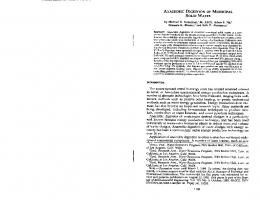
be interpreted as qualitative states. In the example described here, the landmarks result from expert knowledge; e.g., a level can be qualitatively characterised as “low”, “medium”, or “high”. Figure 1 shows the partition of a three-dimensional space with three landmarks for each dimension.

(1)

l1,3 l1,2

ξ ∈Ξ ⊆ ¡ , Ξ n

where

is

an

n-dimensional

state

space,

ζ = g ( p, t ) , ζ ∈ Ζ ⊆ ¡ m , Ζ an m-dimensional input space and p

a set of parameters. However, it is assumed that we have only a partial knowledge of the initial state ξ ( t0 ) and the input values ζ that can be estimated by the intervals − j

+ j

(ζ , ζ ) ∈ Ζ

2 j

(ξi− , ξi+ ) ∈ Ξ i2 and

(with Ξ i ∈ Ξ and Ζ j ∈ Ζ , i = 1,..., n , j = 1,..., m )

defined by

∀j , ∀t , ζ j− ( t ) ≤ ζ j ( t ) ≤ ζ j+ ( t ) ∀i, ξi− (t0 ) ≤ ξ i (t0 ) ≤ ξ i+ (t0 ) 3.1.2

(2) (3)

Imprecision representation

Let us define ζ < and ζ > according to the values of the derivatives as follows:

(4)

Ξ2 Ξ3

Ξ1

Ξ2 Ξ3

l1,3 l3,3 l3,2

li,1 l2,2 Ξ1

l3,3 l3,2

l1,2 l2,3

Ξ2 Ξ3

li,1 l2,2 Ξ1

l2,3

a) b) c) Figure 1. Translation of a continuous state space (a) by landmarks (b) into a discrete space state (c). The basic ideas are (i) to take the faces of the cells partitioning the state space as discrete states (not the cells themselves) and (ii) to determine the transitions between states from the analysis of an output of the continuous system simulated within each cell, as it is done in [4]. Using such an approach, Kowalewski et al. defined a grid on each cell’s faces and simulated all the trajectories issued from or bounded to each grid-point. In comparison, our approach is focused on the propagation of the interval ξ − , ξ +  within each cell by simulating Eqs. (5).

3.3

Trajectories within a cell

Let τ be the time instant when the system (1) reaches v, a landmark value defined in the ith dimension, i.e., ξi (τ ) = v, v ∈ ¡ . Because ξi

Using this approach and performing the synchronised product with Kronos (more details are in [8]) of all the timed automata generated for each dimension of the system, yields a single timed automaton, with one clock without reinitialisation, globally representing the system dynamics for the simulated period. The complete procedure can be found in [13].

is estimated by the interval ξi− , ξi+  , the time window of crossing the v landmark can be described by τ − and τ + such that ξi− (τ − ) = ξi+ (τ + ) = v .

4 APPLICATION TO DIGESTION PROCESS

3.3.1

Landmark crossing

( ( ) ) ( ( ) ) (ξ& (τ )< 0 ) ∧ (ξ& (τ )< 0) ⇒ τ > τ .

From Eqs. (5), it comes: ξ&i− τ − > 0 ∧ ξ&i+ τ + > 0 ⇒ τ + < τ − and − i

−

+ i

+

+

−

Let τ min = min(τ − ,τ + ) , τ max = max(τ − ,τ + ) and F the map that

AN

ANAEROBIC

The above described procedure is applied to an anaerobic digestion process used in wastewater treatment. The aim is to forecast the possible dysfunctions of the process by using a discrete approximation of a mechanistic model together with partial knowledge of the system’s dynamics and parameters.

associates a label to each landmark crossing defined by:

4.1

" v ∆ " if τ min = τ + F (v) →  ∇ − " v " if τ min = τ

(7)

with the symbols ∆ and ∇ denoting landmark crossing with increasing and decreasing trends, respectively. 3.3.2

Timed automaton representation

The system trajectory between two landmarks w and v is represented by the time window τ min ,τ max  which can be modelled in the timed automata formalism (cf. figure 2 where w < v) by: • s1 and s2, two locations with associated propositions " w ∆ " and " v ∆ " respectively, • x, a clock, • x ≤ τ max , the invariant of s1,

( s1 , ∅, x ≥ τ min , ∅, s2 ) , the edge.

•

Ξi

ξi+

s1 "w∆" x ≤ τ max

w

Figure 2.

3.4

Anaerobic digestion is a biological process used for carbon removal from wastewater. The principle is to transform organic matter into biogas (i.e., a mixture of methane CH4 and carbon dioxide CO2) in absence of oxygen. This process has advantages like: • methane may be used as a renewable energy source, • sludge production is low, • anoxic reactions have a low energetic demand. The Laboratory of Environmental Biotechnology of INRA in Narbonne (France) runs a 1 m3 fixed-bed anaerobic reactor since 1997 [14]. This semi-industrial pilot has been used for modelling, diagnostic and control purposes. This complex process involves many parallel and serial reactions that consume a substrate by means of a succession of bacteria communities. However, the process can be summarised by (i) an acidogenic phase, where a first bacterial biomass (X1) converts organic matter (S1) into volatiles fatty acid (VFAs, S2) and (ii) a methanogenic phase, where another biomass (X2) converts S2 into methane and CO2:

ξi−

v

τ+

Process description

τ−

x ≥ τ min

t

Timed automaton representing a trajectory from landmark w to v.

Global timed automaton

Starting from a simulation run of the continuous model on a defined period of time, for each dimension, the continuous system dynamics is approximated by a timed automaton where: • each landmark crossing is assigned a location and a proposition with crossing characteristics and trend by means of Eq. (7), • invariants are defined by the latest time points τ max at which landmark crossing may occur, • guards of edges are defined by the earliest time points τ min at which landmark crossing may occur, • the clock set is a singleton.

r1 k1S1  → X 1 + k2 S 2 + k4CO 2 r2 k3 S 2  → X 2 + k5CO 2 + k6CH 4

s2 "v∆"

(10) (11)

with k1- k6 the yield coefficients and r1, r2 the reaction rates.

4.2 4.2.1

Process model Mass-balance model

A classical mass-balance analytical model is used [15]:  X& 1   X& 2 &  S1 &  S2 & Z C& 

= ( µ1 − α D ) X 1

= ( µ2 − α D ) X 2

= D ( S1in − S1 ) − k1µ1 X 1

= D ( S 2in − S 2 ) + k2 µ1 X1 − k3 µ 2 X 2

(12)

= D ( Z in − Z )

= D ( Cin − C ) − qCO2 + k4 µ1 X1 + k5 µ 2 X 2

with Z the total alkalinity, C the total inorganic carbon concentration, qCO2 the molar flow of CO2, D the dilution rate by

the input flow, α the fraction of bacteria in the liquid phase, k1 to k6 the yield coefficients of the reactions, µ1 and µ2 the growth rate of bacteria in the acidogenic and methanogenic phases and S1in , S2in , Z in and Cin the concentrations of elements in the influent. From this ODE system, and assuming (i) the methane molar flow is only dependent upon the methanogenic biomass activity, (ii) the biogas is mainly composed of methane and CO2 and (iii) the ideal gas law, the following variables can be determined: qCH 4 = k6 µ 2 X 2

(14)

qgas = qCH 4 + qCO2

(15)

k6 µ2 X 2 PCO2

(16)

qCO2 =

PT − PCO2

COD = S1 + kC S 2

4.2.3

The off-diagonal elements of the Jacobian matrix of (19) are ∂f (ξ , ζ , t ) always positive or null apart of 4 for which the condition ∂ξ 2 PCO2 PT

of CO2, COD, the chemical oxygen demand and kc, a conversion constant. Model simplification

type kinetics (inhibition of the reaction by S2 is assumed), we use S2 here a Monod-type kinetics in the form µ2 = µ 2max no S2 + K S2

Given that

Finally Eqs. (13-17) are rewritten to yield:

 S&1   S& ξ =  &2 Z C& 

(18)

with k P = k5 − k6

= D ( S1in − S1 ) − k1µ1 X 1

= D ( S 2 in − S 2 ) + k2 µ1 X 1 − k3 µ 2 X 2 = D ( Z in − Z )

(19)

= D ( Cin − C ) + k4 µ1 X1 + k P µ 2 X 2

PCO2 PT − PCO2

. ψ = g (ξ , ζ , t ) is defined by:

COD = S1 + kC S 2  PT ψ = q = k6 µ 2 X 2  gas P − PCO2 T 

(20)

) ) ) )+k µ

= D S1+in − S1+ − k1µ1+ X 1− = D S 2+in − S2+ + k2 µ1+ X1+ − k3 µ 2+ X 2− + in

− Z+

+ in

− C+

( = D(S = D(Z = D (C

4

+ 1

X1+ + kP µ2+ X 2+

) −S )+k µ X −Z ) −C )+k µ X

(22)

= D S1−in − S1− − k1µ1− X 1+ − 2in − in − in

− 2

2

− 1

− 1

− k 3 µ 2− X 2+

4

− 1

− 1

+ kP µ 2− X 2−

−

−

∀i, ξi− ( t ) ≤ ξ i ( t ) ≤ ξ i+ ( t ) , Eqs. (20) can be

COD +  + qgas    COD −  − qgas  

the half-saturation constant associated to S2. The acidogenic growth rate µ1 is also taken as a Monod-type kinetics

where ξ T = S1 , S 2 , Z , C  , ξ ∈ ¡ 4+ , ψ T =  DCO, q gaz  , ψ ∈ ¡ 2+ and ζ T =  S1in , S 2in , Z in ,Cin , D, PCO2  , ζ ∈ ¡ 6+ . ξ& = f (ξ , ζ , t ) is defined by:

(21)

approximated by :

inhibition), with µ2max the maximum bacterial growth rate and K S2

 ξ& = f (ξ ,ζ , t )  ψ = g (ξ , ζ , t )

( ( = D(Z = D (C

 S&1+   S&2+  +  Z&  &+ C    S& −  1  S&2−   Z& −  &− C

(17)

Using the model and introducing imprecision in it require that simplifications are made to comply with the property (6). First of all, with respect to the length of the simulation period (some hours or some days), the biomasses X1 and X2 are assumed to be constant. Moreover, if in [15], the growth rate µ2 is modelled by a Haldane-

 k5  ≤    k5 + k 6 

must be checked. Note that condition (21) depends only on parameters and inputs. Subject to the satisfaction of condition (21), the ODE system (19) is cooperative, so, it is possible to bound by intervals the input concentration values and obtain:

with PT , the total pressure in the reactor, PCO2 , the partial pressure

4.2.2

Construction of the system bounds

4.3 4.3.1

= S1+ + kC S 2+ = k6 µ 2+ X 2+

PT PT − PCO2

(23) = S1− + kC S 2− = k6 µ 2− X 2−

PT PT − PCO2

Discrete abstraction and analysis of the model Input and initial state of the system

To forecast possible dysfunctions of the plant, it is possible to verify reachability and safety properties so as to envisage the intervention of an operator when the system is potentially in a critical state. Let us assume that the process is in a given situation and that the following events are expected (cf. figure 3): • day 1, low dilution rate and low input concentrations, • day 2, high dilution rate and low input concentrations, • day 3, high dilution rate and high input concentrations, • day 4, low dilution rate and low input concentrations, Based on expert knowledge, the following relations are used to determine PCO2 (with k5 and k6 values, condition (21) is satisfied): D ≤ 0.04 ⇒ PCO2 = 0.2mmol.L-1 D > 0.04 ⇒ PCO2 = 0.3mmol.L-1

(24)

150

100

5 48

72

50

96

Zin 200 100

48

72

96

24

48

72

96

Cin 40 20 0

l∇4,1

COD

l∇5,1

qgas

l∇6,1

0

24

48

24

Figure 3.

48

0 0

72 96 time (h)

Forecasted profiles of inputs used during the experimentation on the process.

Landmarks and associated qualitative states

Figure 4 shows the qualitative states associated with the intervals defined by the landmarks assigned to the state variables domains. The functioning aims are: • COD concentration (representing the residual pollution after treatment) should be low or normal, • biogas production should be sufficient to be further used, • organic overload due to a high substrate concentration S2 should be avoided as it denotes a process dysfunction. Functioning criteria are established by expert knowledge using the qualitative states defined in figure 4. So, the COD concentration allows the following relations to be established: • normal COD, normal S2, and normal qgas: normal functioning of the reactor, • low COD: underload, a bigger quantity of organic matter could be treated, • high COD: the process does not manage well to treat the whole organic matter, pollution still remains after treatment, • critical COD: an important pollution is present in the effluent. The VFAs concentration allows organic overload risks to be defined: • normal S2: very small risk, • high Z and high S2: small risk, • high Z and critical S2: risk, • low Z and high S2 important risk, • low Z and critical S2: very important risk. The production of biogas influences the possibilities of using the energy produced by the process: • low qgas: small production of gas, • high C and high qgas: normal production of gas, • high C and critic qgas: normal production of gas, but possible difficulty for its use (the quality of the biogas may be altered), • low C and high qgas: problematic production of gas, difficulty for its use (biogas composition may be modified), • low C and critic qgas: critical production of gas, significant risk during its use.

normal

l∆2,1

l∆2,2

low

∆ l3,1

low

l∆6,1

l∇5,2

low

2

high

l∇3,2

low

l∆4,1 ∆ l5,1

50

l∇2,2

l∇4,2

l∇2,3

100

critical

l∆2,3

100

l∆3,2

high

75

l∆4,2

high

l∇2,4

l∇3,3 l∇4,3

∞ ∞ ∞

l∆2,4 l∆3,3 l∆4,3

normal 5 ∆ high 10 ∆ critical ∞ ∆ ∆ l5,5 l5,2 l5,3 l5,4 l∇5,3 l∇5,4 l∇5,5 l∇6,2

200

l∆6,2

normal

l∇6,3

400

l∆6,3

high

l∇6,4

∞

l∆6,4

Landmark on different state variables with associated propositions.

Timed automaton approximation

The results of four-day simulations with and without imprecision are shown in figure 5 together with experimental data obtain from the pilot plant. If the simulation without imprecision crosses landmarks sometimes earlier or later than on-line data, the double system (23) allows an imprecise but a good and correct estimation of the process features. The model with imprecision intervals is thus more robust for state prediction. The resulting timed automaton has 1152 locations and 4608 transitions but the set of reachable states has only 118 elements. All the procedure is achieved in 26 seconds on a 1.6 GHz/Windows 2000 computer. 12 gCOD. L-1

h-1

S1in, S2in, Zin, Cin : Upper bound Lower bound

0.02

0

72 96 time (h)

4.3.3

0.04

0

C

0

Figure 4.

D

0.06

4.3.2

24

9

250

S1

S2

6 3

0 0 270

24

48

72

100 50 0 0 200

96

Z

mmol. L-1

0 0 0.08

0

0

60

l∇3,1

0

mmol. L-1

24

Z

50 0 25

24

48

72

96

24

48

72

96

C

100

gCOD. L-1

mmol. L-1

0 0 300

l∇2,1

mmol. L-1

10

S2

24

48

72

96

COD

75 0 0 600

mmol.h-1

15

∞

0 S1

S2in

mmol. L-1

S1in

mmol. L-1

gCOD. L-1

25 20

qgas

400

10 5 2 0 0

200

24

48

72 96 time (h) Upper bound simulation Lower bound simulation On-line data

Figure 5. 4.3.4

0 0

24

48

72 96 time (h) Model’s simulation without intervals (i.e., without imprecision representation)

Model simulation.

Property checking

Table 1 presents the results of checking the properties enumerated in § 4.3.2. The time of reachability of some state is calculated by the model-checker itself (see [13] for more details). For example, in the first line of Table 1, checking the reachability of the state “normal COD, normal S2, and normal qgas” is expressed by:

(l

2,0

)

((

) (

) (

∆ ∆ ∆ ∧l5,0 ∧l6,0 ⇒ ∃◊ l2,1 ∨ l∇2,2 ∧ l5,2 ∨l∇5,3 ∧ l6,2 ∨ l∇6,3

))

(26)

where li∆, j and l∇i , j represent crossing of landmark j in the ith dimension, respectively with increasing and decreasing trends. Eq. (26) means, “from the initial state, is it possible to reach a state corresponding to normal COD (i.e., between landmark 1 and 2), normal S2 (i.e., between landmark 2 and 3), normal qgas (i.e., between landmark 2 and 3)?” (cf. figure 4). The same approach is used to check all the properties listed in Table 1. Table 1.

Property checking on the four-day period. Properties

normal COD, normal S2, and normal qgas low COD high COD critical COD normal S2 high Z and high S2 high Z and critical S2 low Z and high S2 low Z and critical S2 low qgas high C and high qgas high C and critic qgas low C and high qgas low C and critic qgas

State reachability times (hours) [24 49] and [84 96] [0 26] and [94 96] [28 59] and [76 96] [47 96] [0 54] and [81 96] [32 96] [51 96] [32 50] unreachable [0 50] and [83 96] [53 96] [53 96] [24 79] [47 79]

But it is also possible to check properties like “the system is always in a normal state” by checking the reachability of the negation of the normal states:

(l

2,0

)

((

) (

) (

∆ ∆ ∆ ∧l5,0 ∧l5,0 ⇒ ∃◊¬ l2,1 ∨l∇2,2 ∧ l5,2 ∨l∇5,3 ∧ l6,2 ∨ l∇6,3

))

(27)

Model-checking allows us to verify that this statement is true at all times. As a consequence, no guarantee exists that the system will normally run during the four-day period.

5

DISCUSSION AND CONCLUSION

This paper describes an implemented procedure to abstract the dynamics of a continuous system into a timed automaton, where (i) inputs and initial states are estimated by intervals, which comes down to simulate the system behaviour by simulating its upper and lower bounds represented as an extremal ODE system and (ii) the generated behaviour is transformed into a timed automaton (discrete formalism with continuous time), which is made possible by partitioning the state variables’ domains by landmarks according to expert knowledge. The principal characteristics are to take landmark crossing as discrete states and to use this procedure with an initial state, imprecise inputs and a landmark definition set. The final size of the automaton depends upon the system’s dimension, the number of landmarks and landmark crossings. Consequently, this approach is inappropriate when the system oscillates around a landmark value and if a large number of landmarks are defined. Nevertheless, this approach has been devised to be executed "on the fly" when one wishes to verify a specific property of a continuous system. The idea is not to create an automaton that can check all the possible properties but, rather,

to create an automaton according to the property to be checked by defining adequate landmarks. It was shown how this approach can be used to forecast qualitative states of a real anaerobic digestion process by approximating an analytical mass-balance model. An interesting extension would be to couple this representation to the discrete part of a hybrid dynamical system in order to check properties on mixed continuous and discrete elements.

ACKNOWLEDGEMENTS This work was partially supported by the Région Réunion and the European Social Fund.

REFERENCES [1] P. Struss. ‘Automated Abstraction of Numerical Simulation Models Theory and Practical Experience’, proceedings of Model Based Systems and Qualitative Reasoning for Intelligent Tutoring Systems, 161-168, (2002). [2] M.-O. Cordier and C. Largouët. ‘Using model-checking techniques for diagnosing discrete-event systems’. proceedings of DX'01, International Workshop on Principles of Diagnosis, (2001). [3] P. Supavatanakul, C. Falkenberg and J. Lunze. ‘Identification of timed discrete event models for diagnosis’, proceedings of DX'01, International Workshop on Principles of Diagnosis, (2003). [4] S. Kowalewski, S. Engell, J. Prußig and O. Stursberg. ‘Verification of logic controller for continuous plants using timed condition/eventsystem models’, Automatica, 35, 505-518, (1999). [5] T. A. Henzinger, P.-H. Ho and H. Wong-Toi. ‘Algorithmic Analysis of Nonlinear Hybrid Systems’. IEEE Transactions on Automatic Control, 43, 540-554, (1998). [6] R. Alur and D. Dill. ‘The theory of timed automata’, Theoretical Computer Science, 126, 183-235 (1994). [7] T. A. Henzinger, X. Nicollin, J. Sifakis and S. Yovine. ‘Symbolic Model Checking for Real-Time Systems’, Information and Computation, 111, 193-244, (1994). [8] S. Yovine. ‘Kronos: A verification tool for Real-Time Systems’, Journal of Software Tools for Technology Transfer, 1, 123-133, (1997). [9] P. Pettersson and K. G. Larsen. ‘Uppaal2k’, Bulletin of the European Association for Theoretical Computer Science 70, 40-44, (2000). [10] K. G. Larsen, P. Pettersson and W. Y. I. Springer. ‘UPPAAL in a Nutshell’, International Journal of Software Tools for Technology Transfer, 1, 134-152, (1997). [11] H. L. Smith. ‘Monotone dynamical systems: An introduction to the theory of competitive and cooperative systems’, AMS Mathematical Surveys and Monographs, 41, 31-53, (1995). [12] J. L. Gouzé, A. Rapaport and M. Z. Hadj-Sadok. ‘Interval observers for uncertain biological systems’, Ecological Modelling, 133, 45-56 (2000). [13] A. Hélias. ‘Agrégation/abstraction de modèles pour l'analyse et l'organisation de réseaux de flux : application à la gestion des effluents d'élevage à la Réunion’, PhD thesis, ENSAM, Montpellier (France), (2003). [14] J.-P. Steyer, J.-C. Bouvier, T. Conte, P. Gras and P. Sousbie. ‘Evaluation of a four year experience with a fully instrumented anaerobic digestion process’, Water Science and Technology, 45, 495502, (2002). [15] O. Bernard, Z. Hadj-Sadok, D. Dochain, A. Genovesi and J.-P. Steyer. ‘Dynamical model development and parameter identification for anaerobic wastewater treatment process’, Biotechnology and Bioengineering, 75, 424-438 (2001).