Application to User Interface Design - People @ EECS at UC Berkeley

Invariance-Preserving Abstractions of Hybrid Systems: Application to User Interface Design∗ Meeko Oishi1 , Ian Mitchell2 , Alexandre Bayen3 , Claire Tomlin4 1

American Institute of Biological Sciences, Washington, DC, USA [email protected]

2

Dept. of Computer Science, University of British Columbia, Vancouver, BC, Canada [email protected] 3

Civil Engineering, University of California, Berkeley, CA, USA [email protected]

4

Dept. of Aeronautics and Astronautics, Stanford University, Stanford, CA, USA [email protected] November 8, 2005

Abstract Hybrid systems combine discrete state dynamics which model mode switching, with continuous state dynamics which model physical processes. Hybrid systems can be controlled by affecting both their discrete mode logic and continuous dynamics: in many systems, such as commercial aircraft, these can be controlled both automatically and using manual control. A human interacting with a hybrid system is often presented, through information displays, with a simplified representation of the underlying system. This user interface should not overwhelm the human with unnecessary information, and thus usually contains only a subset of information about the true system model, yet, if properly designed, represents an abstraction of the true system which the human is able to use to safely interact with the system. In safety-critical systems, correct and succinct interfaces are paramount: interfaces must provide adequate information and must not confuse the user. We present an invariance-preserving abstraction which generates a discrete event system that can be used to analyze, verify, or design user-interfaces ∗ Research supported by a National Science Foundation Graduate Research Fellowship, by DARPA under the Software Enabled Control Program (AFRL contract F33615-99-C-3014), by the DoD Multidisciplinary University Research Initiative (MURI) program administered by the Office of Naval Research under Grant N00014-00-1-0637, and by Grant NCC2-798 from NASA Ames Research Center to the San Jose State University Foundation, as part of NASA’s base research and technology effort, human-automation theory sub-element (RTOP 548-40-12).

1

for hybrid human-automation systems. This abstraction is based on hybrid system reachability analysis, in which, through the use of a recently developed computational tool, we find controlled invariant regions satisfying a priori safety constraints for each mode, and the controller that must be applied on the boundaries of the computed sets to render the sets invariant. By assigning a discrete state to each computed invariant set, we create a discrete event system representation which reflects the safety properties of the hybrid system. This abstraction, along with the formulation of an interface model as a discrete event system, allows the use of discrete techniques for interface analysis, including existing interface verification and design methods. We apply the abstraction method to two examples: a car traveling through a yellow light at an intersection, and an aircraft autopilot in a landing/go-around maneuver.

1

Introduction

Human-automation interaction is pervasive, occurring in consumer products (alarm clocks, VCRs, cellular phones), transportation systems (automobiles, commercial aircraft, air traffic control), scientific research platforms (unmanned ocean- and aerial-vehicles), and military systems (fleets of semi-autonomous and autonomous aircraft), among others. Often complicated by the underlying dynamics of the physical system, human-automation interaction in aviation has been a controversial topic since the advent of computers and their integration into the cockpit [1, 2, 3]. The aviation industry has experienced many incidents and some accidents in which the pilot became confused about the current mode or could not anticipate the next mode in the automation [4, 5, 6, 7]. This potentially dangerous problem has been loosely termed mode confusion, and is often addressed in flight when the pilot has the time to devote attention to it, and resolved later with ad-hoc “fixes”. However, mode confusion may occur at critical times of flight: In 1994, all seven people on-board died during a test flight of the A-330 in Toulouse, France [8, 9]. The pilot had attempted to complete a go-around with a simulated engine failure, but an unanticipated combination of aircraft and engine dynamics, flight envelope protection schemes, and confusing interface indications led to the aircraft’s stall. The accident involved the aircraft’s software, aerodynamics, as well as the pilot’s interaction with the combined system. We focus specifically on an aspect of this problem which we can quantify: the information content presented in the interface. While graphical design of the interface is key in determining how the user processes and interacts with information in the interface, we assume that the user can and does process all information displayed. In human-automation systems, the interface allows observation of information regarding the underlying system dynamics and processes, as well as control over specific behaviors through input devices in the interface. Too much information can

2

overwhelm the user; with too little information the user may not understand the system’s behavior or may not be able to perform the desired task. A key part of the problem of interface design and verification involves the appropriate selection of information from the underlying human-automation system which should be displayed to the human controlling the system. Although the engineering psychology community has historically dominated research on humanautomation interaction, there have recently been efforts by the formal methods community [10, 11, 12, 6, 13] as well as systems and control communities [14, 15] to address these safety-critical problems. Using model checkers, researchers in formal methods have evaluated such interfaces to identify design problems [10, 11, 16] for discrete state models. In [12, 17, 18], the authors were not only able to verify interfaces for a given task, but additionally formally determine the minimum set of information that must be displayed in the cockpit interface in order to safely complete a given maneuver. We believe that the continuous dynamics plays a crucial role in understanding and designing interfaces, and that it is necessary to introduce both a continuous dynamic component to represent the physical dynamics of the underlying system, and a control component, into previously proposed methodologies to make them sound techniques for physical systems. We model complex human-automation systems as hybrid systems over which a human shares control with automation. In this framework, which establishes a new way of modeling human interaction with automation, we determine how to abstract, from the hybrid system, a reduced representation of the underlying system. This representation can then be used in existing discrete interface verification or design algorithms. The particular representation which we construct addresses the problem of system safety, in which we consider a system to be safe if it fulfills a certain mathematical property which can be encoded as a condition on the system’s reachable set of states. In aircraft, for example, a safe system is one which remains within its aerodynamic flight envelope. This contribution differs from existing work in hybrid system verification in our treatment of the user’s interactions with the hybrid system. One of the key enabling technologies human-automation systems is verification, which allows for heightened confidence that the system will perform as desired. Verification is defined simply as the process of developing and executing a mathematical proof that a system model satisfies a given specification. Methods and tools to verify systems have become very important as the complexity of automated systems has grown; it is no longer possible to rely on intuition and simulation to test that a system satisfies its specification. Verification tools can aid in drastically reducing time spent on design and validation, but are also crucial in ensuring that safety properties are upheld. In safety-critical, expensive, or high-risk applications such as airbag deployment circuitry, aircraft autopilots, and medical devices, guarantees of safe operation are paramount.

3

Hybrid reachability analysis and controller synthesis address the problem of guaranteeing system safety. Many problems of interest may be posed as reachability specifications. For example, in the problem of verifying system safety, the safety specification is first represented as a desired subset of the state-space in which the system should remain, and then the following reachability question is posed: Do all trajectories of the system remain within this set of desired states? The process of verifying safety then involves computing the subset of the state-space which is backwards reachable from this “safe set” of states. If this backwards reachable set intersects any states outside the desired region, then the system is deemed unsafe. Controller synthesis for safety is a procedure through which one attempts, by restricting the behavior of the system through a controller, to prune away system trajectories which lead to unsafe states. In the past several years, methods and tools have been developed for computing reachable sets for continuous and hybrid systems [19, 20, 21, 22, 23]. Many of these approximate the continuous dynamics and use an over-approximative set representation in order to maintain computational tractability for high dimensional systems. In this paper, we use a time-dependent Hamilton-Jacobi formulation [24] for specifying the reachable set, and the corresponding numerical toolbox based on level set methods [25, 26, 27] for computing the reachable set. This technique works for general nonlinear dynamics and set representation. Previous work in analyzing hybrid system safety, for example [28], has focused on applications of hybrid system theory to fully automated systems, assuming that the controller itself is an automaton. Here we consider the problem of controlling human-automation systems, in which the automaton and a human controller share authority over the control of the system [7]. The user interacts with the underlying system through an interface, a reduced description of the behavior of the system. In particular, we consider the problem of verification of an interface between a semi-automated hybrid system and a human controller, and we pose the question: Is the information displayed to the human controller about the hybrid system evolution sufficient for the human controller to act in such a way that the system remains safe? In previous work [15] we focused on one particular example in which verification that an interface correctly represented the underlying hybrid system was paramount: the automatic landing of a large civil jet aircraft. Here, we generalize the abstraction technique which allowed us to make use of discrete interface verification tools. We analyze the user-interface of a hybrid human-automation system based on well-developed tools in the realm of hybrid system reachability analysis. These tools assume a hybrid model of the human-automation system (which includes how the user interacts with the system). We create a discrete representation of the hybrid model based on the hybrid system reachability result, from which we can then design an appropriate interface for the hybrid system. In cases in which we are given an interface which can be represented as a discrete system,

4

the task, then, is to verify the safety of the discrete interface using the discrete representation of the hybrid human-automation system. The paper is organized as follows: We first introduce the modeling formalism, and describe the particular way in which we model human interaction with a hybrid system. We then describe a method to create the discrete invariance-preserving abstraction, and apply it to two examples, in which correct interface design requires information drawn from the underlying hybrid dynamics. We first present an everyday example: driving on an expressway through a yellow light, and show how, with this method, an interface can be constructed based on the reachability result of the underlying hybrid system. After discussing the abstraction method, we present a more complicated example: the automatic landing of a civil jet aircraft, without the simplifications taken advantage of in [15]. Lastly we offer some conclusions and directions for future work.

2

Problem Description

2.1

Problem Formulation

Consider a hybrid system H = (Q, X , R, f, Σ, U) defined by: • the set of discrete modes Q, • the domain of continuous states X , • the transition function R : Q × Σ × X → Q × X , • the functions fq (x, u) : Q × X × U → X , • the set of discrete inputs, or events Σ = Σ u ∪ Σh ∪ Σd , • and the set of continuous inputs U, We assume that discrete controlled inputs σ u ∈ Σu are initiated by an automated controller (e.g. an automatic transition based on the continuous state), discrete human-initiated events σ h ∈ Σh are initiated by the human (e.g. pushing a button, toggling a lever), and discrete disturbance inputs σd ∈ Σd are initiated by something external to the system (e.g. a fault, caused neither by the automatic controller nor the human). We index the continuous dynamics by the current discrete mode, so that x˙ = fq (x, u), with x ∈ X ⊆ Rn and u ∈ U ⊆ Rm in mode q ∈ Q. We assume that the continuous input is controlled automatically. While we anticipate that the method presented in this paper can be extended to treat systems with continuous disturbances or continuous human inputs, these issues are not addressed here. Additionally, the initial set is (Q 0 , X0 ) and the constraint set is C = (Q, W0 ) ⊆ Q × X . The constraint set represents the desired subset of the state-space in which the system should remain. We index the continuous constraint set in mode q by W 0 (q), i.e. (q, W0 (q)) ⊆ C. 5

ˆ = (Q, ˆ Σ, ˆ R), ˆ defined by Let us also consider a discrete event system G ˆ • the set of discrete modes Q, ˆ:Q ˆ ×Σ ˆ → 2Qˆ , and • the transition relation R ˆ =Σ ˆu ∪ Σ ˆh ∪ Σ ˆ d. • the set of events Σ The event set contains controlled, human-initiated, and disturbance events. The set of initial modes ˆ 0 , and the constraint set is Cˆ ⊆ Q. ˆ is Q Definition 1 A hybrid system H, defined as above, for which Σ h 6= ∅, is called a hybrid humanautomation system. Definition 2 For a trajectory to be invariant with respect to a constraint set C, it must begin within, and always remain within C. Definition 3 For a trajectory to be user-invariant with respect to a constraint set C, it must begin within C, and may exit C only under human inputs. ˆ is invariance-preserving with respect to the constraint set Definition 4 A discrete event system G ˆ that are invariant or user-invariant. C if it accepts only trajectories of G ˆ is a discrete event system representation of Definition 5 An invariance-preserving abstraction G ˆ is invariance-preserving. a hybrid system H with constraint set C, for which discrete event system G Problem 1 Given a hybrid human-automation system H, and a constraint set C, find an invarianceˆ of H. preserving abstraction G ˆ can be compared to an existing discrete interface through The invariance-preserving abstraction G ˆ interface , a a discrete verification procedure; or it can be used to synthesize a discrete interface G ˆ which a user can use to safely interact with the underlying system H. The reduced version of G majority of work on abstractions (see, for example, [29, 30, 31, 32, 33, 34, 35]) makes use of discrete abstractions to aid in continuous or hybrid verification, often by exploiting certain properties of the system (for example, polynomial or bounded continuous dynamics). The invariance-preserving abstraction we propose here can take place after reachability analysis has been used to determine sets of initial conditions which produce invariant trajectories. Rather than aiding in the verification process, this is a post-processing step in which a discrete automaton is formed based on the verified system. In our formulation of a hybrid human-automation system, human-initiated input occurs through discrete inputs. The human may influence the hybrid system trajectory, but does not have to. For 6

example, consider (qk+1 , x) = R(qk , x, σh ), in which the human may initiate a transition σ h which switches the mode from qk to qk+1 . The human controls not only when, but if the transition occurs at all. If the human does not initiate σ h , then the system will remain in qk unless other statebased or disturbance transitions exist which will allow the system to exit mode q k . This nicely models applications such as flight management systems, in which the pilot may initiate high-level mode-changes and the flight management system maintains low-level control.

2.2

Illustration: Advisory System for the Yellow Interval Dilemma

Consider the following scenario: As a single driver on an expressway approaches an intersection, suddenly the light turns yellow. The driver must decide whether to brake and try to stop at the intersection, or to continue driving through the intersection before the red light appears. In either case, the driver must avoid a red light violation, which occurs whenever the car is in the intersection at any time during a red light. Typically, due to several factors, including accumulated experience about the particular car’s braking capabilities, the duration of the yellow light at a given intersection, and the road and weather conditions, the driver has an “intuitive” feel for the correct course of action [36]. At some intersections, despite the driver’s best intentions, there are certain combinations of speed and distance from the intersection for which a red light violation is inevitable: this is known as the yellow interval dilemma [37, 38]. We wish to design an add-on advisory system, whose interface would indicate to the driver which action must be taken in order to avoid a red light violation. We assume a point-mass model of the car without the additional complexity of gearing [39]. With position x from the near-side of the intersection and speed v = x, ˙ braking and acceleration forces enter through x ¨ = u. The car has limited braking and acceleration capabilities (u ∈ [umin , umax ]) and must obey the speed limit at all times (v < v max ). For this scenario, umin = −4m/s2 , umax = 2 m/s2 , and vmax = 24m/s. The intersection is 10 m in length, and the duration of the yellow light is ∆ = 4 seconds [40, 37]. A typical driver’s reaction time after seeing the yellow light is τ = 1.5 seconds [36, 40, 41], during which time we presume the car travels at its present speed. The advisory system should be designed with the assumption that the driver will take one of two courses of action when a yellow light appears: 1) accelerate through the intersection (without violating the speed limit), or 2) brake to stop at the intersection. The question we wish to answer is: What actions does the driver need to take, and when should the driver enact them, in order to avoid a red light violation? Consider the hybrid model Hcar with continuous state x = [x, v, t]T , shown in Figure 1, in which 7

t≥0∧ σbrake

Hgreen δ, t := 0

qgreen »

x˙ v˙

–

=

»

v u

–

t˙ = 1 u ∈ [umin , umax ] x ∈ Xgreen

brake qyellow

»

qyellow »

x˙ v˙

–

=

»

v u

t˙ = 1 u=0 x ∈ Xyellow

–

t≥0∧ σaccel

x˙ v˙

–

=

»

v u

t˙ = 1 u=0 x ∈ Xyellow

accel qyellow

»

x˙ v˙

–

=

»

brake qreact

t≥τ –

»

x˙ v˙

v u

t˙ = 1 u=0 x ∈ Xyellow

=

»

v u

accel qreact

»

x˙ v˙

–

=

»

brake qred

t≥∆ –

t˙ = 1 u = [umin , umax ] x ∈ Xyellow

t≥τ –

–

»

x˙ v˙

v u

t˙ = 1 u = umax x ∈ Xyellow

=

»

v u

–

brake Hyellow

–

accel Hyellow

t˙ = 1 u = [umin , umax ] brake x ∈ Xred

accel qred

t≥∆ –

–

»

x˙ v˙

–

=

»

v u

t˙ = 1 u ∈ [umin , umax ] accel x ∈ Xred

Figure 1: Hybrid model Hcar for a car traveling through an intersection, where the input u is the car’s acceleration, and x := [x, v, t]. brake , q brake , q accel , q accel , q brake , q accel }, • Qcar = {qgreen , qyellow , qyellow react yellow react red red + • Xcar = R × R+ 0 × R0 ,

• Ucar = [umin , umax ], • Σcar = Σu ∪ Σh ∪ Σd , with controlled events Σu = {t ≥ 0, t − τ ≥ 0, t − ∆ ≥ 0} (which are triggered when the inequality is met), human-initiated events Σ h = {σbrake , σaccel }, and disturbance event Σd = {δ}. The event δ represents the light turning yellow. The transition function R car and the continuous dynamics fcar are defined as shown in Figure 1. The initial set is (q green , Xgreen ), and the constraint accel , X brake }, with X set is Ccar = Qcar ×(Wcar )0 , (Wcar )0 = {Xgreen , Xyellow , Xred green = {R×(0, vmax ]× red + + + brake = {(−∞, 0] × (0, v R+ max ] × R0 }, and 0 }, Xyellow = {R × (0, vmax ] × R0 } ∪ {0 × 0 × R0 }, Xred + accel = {[L, ∞) × (0, v Xred max ] × R0 }. The constraint set encapsulates the desired regions of operation

in terms of the car’s position relative to the intersection and the car’s speed: during the red interval, the constraint set is any position outside the intersection and any positive speed, plus the position right at the boundary of the intersection with a speed of 0; during the green and yellow intervals the constraint set is any position and positive speed. ˆ car of the hybrid human-automation sysProblem 2 Find an invariance-preserving abstraction G tem Hcar , given the constraint set Ccar .

3

Creating an Invariance-Preserving Abstraction

In this section, we propose a three-step algorithm to construct an invariance-preserving abstraction ˆ of a hybrid human-automation system H. Each of the three steps in Algorithm 1 will be detailed G

8

ˆ is an in the following sections, followed by a proof that the resultant discrete event system G invariance-preserving abstraction of the hybrid human-automation system H. Definition 6 For every mode q ∈ Q in the hybrid human-automation system H, define the set of modes HumanReach(q) as the set of all modes which could result after any human-controlled transition from q: 4

HumanReach(q) = {p | (p, x) ∈ R(q, x, σh ), for all σh ∈ Σh such that R(q, x, σh ) exists }

(1)

Definition 7 Define the set of entry modes Q entry = {HumanReach(q), q ∈ Q}∪Q0 as the union of those modes which result after any discrete human input and those modes in the initial set. Define 4

the cardinality of the entry modes as N = kQentry k. ˆ of a hybrid human-automation Algorithm 1 To create an invariance-preserving discrete abstraction G system H, 1. Separate the hybrid human-automation system H into N hybrid subsystems H i , using the HumanReach(·) operator to delineate subsystems which contain no human input. ˆ i of hybrid subsystem Hi . 2. For i = 1 : N , compute the invariance-preserving abstraction G ˆ i into one discrete event system G. 3. Combine discrete event systems G

3.1

Step 1: Separation into Hybrid Subsystems

In many human-automation systems, it is important to limit how a human’s actions will be prescribed. We therefore wish to minimize the restrictions placed on the human input through our analysis. We begin our analysis of the human-automation system H by first characterizing regions of H in which human input is impossible. The first step is to decompose H into subsystems which contain no discrete human inputs. As noted earlier, it is impossible to guarantee that a trajectory will be invariant when the system contains human-initiated inputs. However, we can determine regions of the state-space for which invariant trajectories are possible because no human-initiated inputs exist. We accomplish this by isolating modes forward-reachable after a human-initiated transition has occurred, and defining those modes as a subsystem of the original system H. Thus, within each subsystem, all of the transitions are controlled or disturbance transitions. Definition 8 Given an entry mode qi ∈ Qentry , the hybrid system H = (Q, X , R, f, Σ, U), and a constraint set C = (Q, W0 ), define the hybrid subsystem Hi = (Qi , Xi , Ri , fi , Σi , Ui ) as: 9

• Qi is the set of modes reachable from qi through any string of automatic and disturbance events (that is,any string which does not contain a user-initiated event)  R(q, x, σ) if σ ∈ / Σh and q ∈ Qi • Ri (q, x, σ) =  {∅} otherwise • Σi = {σ | Ri (q, x, σ) exists, q ∈ Qi } and Xi , fi , Ui are subsets of X , f, U which correspond to the modes in Q i ⊆ Q. Similarly, the 4

constraint set Ci = (Qi , (Wi )0 ) is a subset of C which corresponds to the modes Q i ⊆ Q. For ease of notation, we label the entry modes q 1 , ..., qN . These indices also label the hybrid subsystems, H1 , ..., HN . The following indexing function associates each mode q ∈ Q to the hybrid subsystems it is contained in: 4

Ind(q) = {i | q ∈ Qi }, where i ∈ {1, ..., N }.

(2)

Note that in general, hybrid human-automation systems will separate into hybrid subsystems which could overlap. Yellow Interval Example:

For the hybrid human-automation system H car , applying Def-

brake , q accel }, since HumanReach(q inition 7 results in entry modes Qentry = {qgreen , qyellow yellow ) = yellow brake , q accel } and Q = {q {qyellow 0 green }. We then apply Definition 8 to find that H car separates into three yellow brake , and H accel , as shown in Figure 1. For example, H hybrid subsystems: Hgreen , Hyellow green contains yellow

Qgreen = {qgreen , qyellow }, Σgreen = {δ}, and Rgreen is graphically depicted in the left-most shaded region of Figure 1. The constraint set for H green is Cgreen = {(qgreen , (Wgreen )0 ), (qyellow , (Wyellow )0 )}. accel The index function Ind maps each mode in Q car to either Qgreen , Qbrake yellow , or Qyellow : for example,

Ind(qyellow ) = green, since qyellow ⊆ Qgreen .

3.2

Step 2: Invariance-Preserving Discrete Abstraction

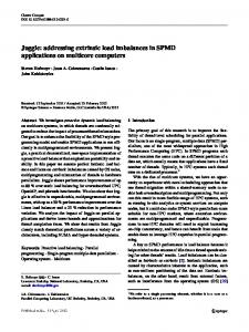
In Step 2 of Algorithm 1, we create an invariance-preserving abstraction of each hybrid subsystem identified in Step 1. Since the hybrid subsystems do not contain any discrete human inputs, standard reachability tools can be used to find invariant sets within each subsystem. Hybrid reachability analysis and controller synthesis provides us with a mathematical guarantee of invariance to within the limits of the hybrid model, through the generation of 1) the invariant set of states, (Q, Wi ) ⊆ Ci contained within the constraint set C i , and 2) a control law which ensures that trajectories which reach the boundary of the invariant set will not be allowed to exit the invariant set (Figure 2). For the reachability computations in Problem 1, any tool can be used which can compute the backwards-reachable invariant set for each hybrid subsystem. This 10

25 vmax

20

v [m/s]

Intersection

15

W(t)

1a 10

W(t) Invariant set at time t

5

Constraint set C = W0 X

0 −120

Figure 2: Constraints on the state-space X are encapsulated in the constraint set C = W 0 . Applying the reachability computation for t seconds, we obtain the invariant set W(t) = φ(C). Trajectories whose initial conditions are contained within W(t) will remain within C for t seconds.

−100

−80

−60

x [m]

−40

−20

0

20

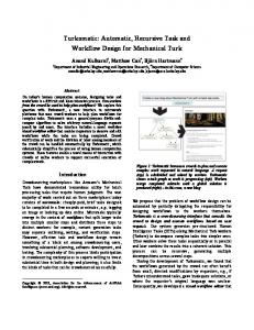
brake Figure 3: Invariant region Wyellow in Hcar in [x, v].

flexibility allows for selection of the hybrid reachability tool most appropriate for the particular system at hand [42, 43, 44, 45, 46, 47]. We use a tool based on level-set methods [26, 27] that computes not only the reachable set, but also the control law necessary to enforce invariance along the boundary of the reachable set. This tool accommodates hybrid systems with general nonlinear continuous dynamics, continuous inputs and disturbances, and discrete inputs and disturbances. Definition 9 An invariant set W ⊆ X has the property that all trajectories with initial state x0 ∈ W are invariant with respect to W. Definition 10 Given a hybrid system H i with Σh = {∅} (no discrete human input), and a constraint set Ci = (Qi , (Wi )0 ), define φ : Qi × (Wi )0 → Qi × (Wi )0 as the result of computing, for t seconds, the invariant set (Qi , Wi ) by means of a backwards-reachable, over- or convergentapproximative numerical tool: φ(C i ) = (Qi , Wi ) ⊆ Ci . Yellow Interval Example:

We compute the invariant sets for each of the constraint sets

brake brake accel in [x, v]: (Qgreen , W) = φ(Cgreen ), (Qbrake yellow , B) = φ(Cyellow ), and (Qyellow , A) = φ(Cyellow ). In each

computed invariant set, we denote the discrete and continuous components as set of pairs of (mode, continuous set): W = {(qgreen , W(qgreen )), (qyellow , W(qyellow )}, for example. The reachability combrake , the putation reveals that W(qgreen ) = W(qyellow ) = Xgreen . In the braking subsystem Hyellow brake ) = B(q brake ) = B(q brake ) = {1a}, the invariant region in each of the three modes is: B(q yellow react red accel , the invariant set A(q accel ) shaded region shown in Figure 3. In the acceleration subsystem H yellow yellow

11

25 vmax

25 vmax

20

20

4

2 2c

0 −120

1 3

10

5

Intersection

2a 10

v [m/s]

2b

v [m/s]

15

Intersection

15

5

−100

−80

−60

x [m]

−40

−20

0

0 −120

20

4 −100

−80

−60

x [m]

−40

−20

0

20

Figure 5: Intersection of invariant sets brake , B) and (q accel , Aaccel ). (qyellow , W), (qyellow yellow yellow

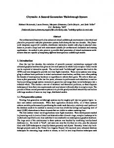
accel accel Figure 4: Invariant set A(qyellow ) ⊆ φ(Cyellow ) in [x, v].

is represented by the three shaded regions, labeled {2a, 2b, 2c} in Figure 4. The invariant set accel ) is represented by {2b, 2c}; and the invariant set A(q accel ) is represented by {2c}. A(qreact red

Proposition 1 Given a hybrid subsystem H i with constraint set Ci , all trajectories whose initial state is contained in the invariant set (Q i , Wi ) ⊆ Ci are user-invariant over time period t. Proof: Proof by contradiction; see Appendix A.1 for details. The only way in which a trajectory that begins in C i can exit Ci is through a human-initiated discrete event: a human-initiated event may transition the system into a state outside of the invariant set in the new mode, such that for (p, x) ∈ C i , R(p, x, σh ) 6⊆ Cj . Denote the complement of a continuous set Wi (p) as Wi (p). Additionally, we presume that trajectories which begin outside the invariant set in one mode (p, x) ∈ (p, W i (p)) evolve to states outside the invariant set in the next mode (q, x0 ) ∈ (q, Wi (q)) for controlled or disturbance events in the hybrid system such that (q, x0 ) = R(p, x, σ), σ ∈ Σu ∪ Σd . Yellow Interval Example: For any trajectory which begins in the shaded region of Figure 3, the car will be able to avoid a red light violation by coming to a complete stop before the intersection. For any trajectory which begins in the shaded region of Figure 4, the car will be able to pass completely through the intersection before the red light occurs. In both cases, computed control laws to enforce invariance must be applied along the boundaries of the shaded sets. ˆ from Definition 11 Given a set of k sets K = {W 1 , · · · , Wk }, Wi ⊆ X , define a map ψ : K → Q the set of k regions in the continuous state-space to the discrete state-space, based on a partition of the continuous domain X . The partition divides X into 2 k disjoint regions {W1 ∩W2 ∩· · ·∩Wk , W1 ∩ 12

W2 ∩· · ·∩Wk , W1 ∩W2 ∩· · ·∩Wk , · · · , W1 ∩W2 ∩· · · Wk ⊆ X } according to the intersection of the sets. Define the set of discrete modes, correspondingly: {w 1 w2 · · · wk , w 1 w2 · · · wk , w1 w 2 · · · wk , · · · , w 1 w2 · · · wk }, so that, for example: ψ

ˆ x ∈ (W1 ∩ W2 ∩ · · · ∩ Wk ) → w1 w ¯ 2 · · · wk 3 Q

(3)

ˆ = ψ(K). The labeling convention of the discrete modes reflects the partiand more generally, Q tioning of the continuous state-space. Definition 11 therefore defines a discrete state-space in which the system being in a particular discrete state corresponds precisely to the continuous state being in the corresponding cell of the state-space partition, according to equation (3). Yellow Interval Example:

4

Consider the intersection of three invariant sets, K yellow =

brake ), A(q accel )}, representing the mode from which a user-initiated transition {W(qyellow ), B(qyellow yellow

is possible, and the two resulting modes. Since W(q yellow ) = Xgreen , we construct the intersection of the remaining two sets, producing 2 2 = 4 disjoint regions in Xgreen . In Figure 5, brake ) ∩ A(q accel ); region {2} represents B(q brake ) ∩ A(q accel ); region region {1} represents B(qyellow yellow yellow yellow brake ) ∩ A(q accel ); and region {4} represents B(q brake ) ∩ A(q accel ). We ab{3} represents B(qyellow yellow yellow yellow

stract these four regions to the discrete modes: wb 1 a1 , wb1 a1 , wb1 a1 , and wb1 a1 , respectively. Let ˆ yellow = {wb1 a1 , wb1 a1 , wb1 a1 , wb1 a1 }, where Q ˆ yellow = ψ(Kyellow ). The result is a set of discrete Q modes which represent the intersection of a set of continuous invariant sets. ˆ Wi ) which selects, for Wi ∈ K, certain modes in Q ˆ = ψ(K), Definition 12 Define a map Sel(Q, created from a partition as defined in Definition 11: 4 ˆ Wi )) = ˆ = ψ(K) for which x ∈ Wi } Sel(Q, {p ∈ Q

(4)

ˆ which represent continuous states for which x ∈ W i . The result is modes in Q Yellow Interval Example: Using the map previously defined, consider the case in which the ˆ yellow which represent driver should brake to a safe stop. We want to select the discrete modes in Q ˆ yellow , B(q brake )) = {wb1 a1 , wb1 a1 }. We now the continuous states from which this is possible: Sel( Q yellow have a discrete representation of the hybrid states (q yellow , x) from which a safe braking maneuver is possible. These definitions are key in creating a discrete abstraction of a hybrid mode. However, beyond constructing the modes of the discrete abstraction (as above), we must also construct the discrete transition relation in a way which mimics the behavior of the original hybrid system. Both of these 13

points are addressed in the following algorithm. In the first step, discrete modes are constructed according to the partition defined in Definition 11. The remaining steps define the discrete transition relation for 1) controlled or disturbance events, 2) human-initiated events, and 3) internal transitions which arise from the continuous dynamics of the original hybrid systems. Algorithm 2 Given a hybrid subsystem H i of the hybrid human-automation system H, a conˆ i as follows: straint set Ci , and an invariant set (Qi , Wi ) = φ(Ci ), create a discrete event system G 1. For each mode p ∈ Qi , uniquely map the continuous state-space (partitioned into 2 K cells, where K = kInd(HumanReach(p))k is the number of distinct modes possible after any humanˆ p corresponding to the hybrid initiated transition from mode p) to a set of discrete states Q state (p, x): ˆ p = ψ({Wi (p), Wk (HumanReach(p))}), k ∈ Ind(HumanReach(p)) Q

(5)

Here, since Hi has no discrete human input, the only states p ∈ Q i for which HumanReach(p) 6= ∅ are the “exit” modes from Qi . ˆ i (ˆ ˆ p , corresponding to the hybrid subsystem transition 2. Define the relation R p, σ) for each pˆ ∈ Q q = Ri (p, x, σ), for p, q ∈ Qi , x ∈ X , σ ∈ Σi (i.e. for those controlled or disturbance transitions 4

to modes within the hybrid subsystem H p ). For ease of notation, denote L = Wi (p) the 4 4 ˆ invariant set Wi in mode p, M = Wi (q) the invariant set Wi in mode q, Pˆ = Q p the set of 4 ˆ ˆ= discrete modes which represent the hybrid state (p, x), and Q Qq the set of discrete modes which represent the hybrid state (q, x).   Sel(Q, ˆ M) for pˆ ∈ Sel(Pˆ , L) ˆ i (ˆ R p, σ) ∈  Sel(Q, ˆ M) for pˆ ∈ Sel(Pˆ , L)

(6)

Because the reachability analysis of Section 2 ensures that for controlled and disturbance events in the hybrid system Hi , trajectories that begin in the invariant set in mode p evolve to the ˆ i is defined invariant set in the following mode q, in Step 2, the discrete transition relation R to reflect this behavior for controlled and disturbance events. See Figure 6 for clarification. ˆ i (ˆ ˆ p , corresponding to any hybrid subsystem tran3. Define the relation R p, σh ) for each pˆ ∈ Q sitions to modes q ∈ HumanReach(p) 6= ∅, for p ∈ Q i , q ∈ Qk , k ∈ Ind(HumanReach(p)), (i.e. for those human-initiated transitions to modes in other hybrid subsystems). For ease of

14

4

notation, denote N = Wk (q) the invariant set Wk in mode q.   Sel(Q, ˆ N ) for pˆ ∈ Sel(Pˆ , N ) ˆ p, σh ) ∈ R(ˆ  Sel(Q, ˆ N ) for pˆ ∈ Sel(Pˆ , N )

(7)

ˆ i is defined such that for human-initiated events, In Step 3, the discrete transition relation R trajectories which begin in the invariant set φ(C i ) in mode p may or may not evolve to the invariant set in the following mode q. This reflects the user’s prerogative to initiate a transition—whether or not the system will be in the invariant set in the next mode depends on the region of the state-space from which the user enacts the switch. See Figure 7 for clarification. ˆ p, αq ) and R(ˆ ˆ q , βq ) for pˆ, qˆ ∈ Q ˆ p , corresponding to movement of the 4. Define the relations R(ˆ continuous state in one mode with respect to the boundary of the invariant set in the next mode q ∈ HumanReach(p) 6= 0, for p ∈ Qi , q ∈ Qk , k ∈ Ind(HumanReach(p)) (i.e. internal transitions not corresponding directly to any discrete transition in H p ). See Figure 7 for clarification. ˆ i (ˆ R p, αq ) = qˆ, with pˆ ∈ Sel(Pˆ , N ) and qˆ ∈ Sel(Pˆ , N ) ˆ i (ˆ R q , βq ) = pˆ,

(8)

ˆ i is defined such that for internal events, it reflects the The discrete transition relation R original continuous dynamics that govern the movement between cells of the partition defined in Definition 11. The controlled event α k occurs when the continuous state exits the region α

k in which a transition to mode q would be invariance-preserving: x ∈ W k (q) −→ x ∈ Wk (q).

Conversely, the controlled event β k occurs when the continuous state enters the region in β

k x ∈ Wk (q). which a transition to mode q would invariance-preserving: x ∈ W k (q) −→

ˆ ˆ i = (Q ˆ i, Σ ˆ i, R ˆ i ), with Q ˆi = S Q ˆ ˆ ˆ The result is G p p , Σi = Σi , and (Qi )0 = Qp , p = (Qi )0 . ˆ i reflects, by construction, the evolution of hybrid system trajectories The discrete event system G with respect to the hybrid invariant sets. ˆ i is invariance-preserving for trajectories whose initial Proposition 2 The discrete event system G ˆ inv )0 = Sel(Wi (p), Q ˆ p ), p = (Qi )0 . states are contained in (Q i

Proof: Proof by induction; see Appendix A.2 for details.

15

αq

ln

βq

ln σh

σh αq

x˙ = fp (x, u) x∈L γ

x˙ = fq (x, u) x∈M Hybrid

l

x˙ = fp (x, u) x∈L σh

l

γ

γ

m

x˙ = fq (x, u) x∈N

m Discrete

Hybrid

βq

ln

σh

σh

n

n Discrete

Figure 7: Discrete abstraction of a two-mode hybrid automaton with human-initiated discrete input σh . The hybrid modes belong to different hybrid subsystems Hi and Hk , therefore p ∈ Qi and q ∈ Qk . The invariant sets are φ(Ci ) = {(p, L)} and φ(Ck ) = {(q, N )}. In the corresponding discrete abstraction, Pˆ = ˆ = {n, n}. {ln, ln, ln, ln} and Q

Figure 6: Discrete abstraction of two-mode hybrid automaton with one controlled discrete input γ. Both hybrid modes belong to the same hybrid subsystem Hi , therefore p, q ∈ Qi . The invariant set is φ(Ci ) = {(p, L), (q, M)}. In the corresponding disˆ = {m, m}. crete abstraction, Pˆ = {l, l} and Q

Yellow Interval Example:

ln

Consider subsystem H green . With no user-controlled transi-

tions HumanReach(qgreen ) = {∅}, the state-space for p = qgreen is partitioned into 21 regions: ˆ green = {W(qgreen ), W(qgreen )}. The abstraction of these two continuous regions is the modes Q ˆ yellow = {wb1 a1 , wb1 a1 , wb1 a1 , wb1 a1 }. {w, w}. Previously we constructed the discrete modes Q Since the transition δ from qgreen to qyellow is a disturbance event, we follow Step 2 of Algorithm 2 to determine the transition function in the discrete abstraction. According to Equation (6) ˆ green , W(qgreen )) and Q ˆ yellow = Sel(Q ˆ green , W(qyellow ), the transition relation is since w = Sel(Q ˆ R(w, δ) ∈ {wb1 a1 , wb1 a1 , wb1 a1 , wb1 a1 }. Now consider mode qyellow . Two transitions are possible, both human-initiated events. If brakbrake ; if acceleration is chosen, the hybrid ing is applied, the hybrid system switches into mode q yellow accel . In the discrete abstraction, these two modes are represented system switches into mode qyellow

by {b1 , b1 } and {a1 , a1 }, respectively, based on reachability analysis performed earlier. Following ˆ brake , B(q brake )) is in the Equation(7) of Algorithm 2, since we know that the mode wa 1 b1 ∈ Sel(Q region of the state-space that

yellow yellow brake is “safe” in the next mode, q yellow , the corresponding relation in the ˆ green (wb1 a1 , σbrake ) ∈ Sel(Q ˆ brake , B(q brake )), which simplifies to as R yellow yellow

discrete abstraction is defined ˆ green (wb1 a1 , σbrake ) = b1 . Similarly, we can find that R ˆ green (wb1 a1 , σbrake ) = b1 . A total of eight R such transitions are defined for the two user-initiated transitions (σ brake and σaccel ) possible from ˆ yellow . The result is depicted in Figure 8. Additionally, internal transieach of the four modes in Q ˆ green (wb1 a1 , αyellow ) = wb1 a1 corresponds tions are shown graphically in Figure 8. The transition R brake to the continuous state evolving from a region in which braking would be a safe course of action,

16

to one where it would not be safe. brake . No user-initiated transitions are Lastly, consider one of the remaining hybrid modes: q yellow ˆ brake = {b1 , b1 }. We again look possible, so we abstract this hybrid mode to 2 1 discrete modes, Q yellow

to Equation (6) of Algorithm 2 to determine the appropriate transition relation in the discrete ˆ brake (b1 , t ≥ τ ) = b2 , R ˆ brake (b1 , t ≥ τ ) = b2 , where Q ˆ brake abstraction: R react = {b2 , b2 }. The discrete ˆ brake = {b3 , b3 }, abstraction of the other modes in Hbrake and Haccel proceeds similarly, with Q red

ˆ accel ˆ accel ˆ accel = {a1 , a1 }, Q Q react = {a2 , a2 }, and Qred = {a3 , a3 }, and similarly defined transition relations yellow in the discrete abstraction, as shown in Figure 8.

3.3

ˆi Step 3: Connecting systems G

The third step of Algorithm 1 is to combine the N abstractions G i into a single discrete event ˆ = (Q, ˆ Σ, ˆ R). ˆ system G S ˆ ˆ = S Q ˆ ˆ ˆ qi , σ) = R ˆ i (ˆ ˆ i , qˆ ∈ Q ˆ i with Definition 13 We define Q q , σ), σ ∈ Σ i i, Σ = i Σi , and R(ˆ

i ∈ Ind(Qentry ).

ˆ car of the hybrid Yellow Interval Example: The invariance-preserving discrete abstraction G system Hcar (Figure 1) is shown graphically in Figure 8. ˆ = (Q, ˆ Σ, ˆ R) ˆ with initial modes Q ˆ 0 , constructed acProposition 3 The discrete event system G cording to the three-step procedure in Algorithm 1 from the hybrid system H = (Q, X , R, f, Σ, U) with constraint set C ∈ Q × X , is an invariance-preserving abstraction of H. Proof: Proof by contradiction; see Appendix A.3 for details.

3.4

Using the Discrete Abstraction

ˆ using existing An advisory system can then be deduced from the invariance-preserving abstraction G discrete reduction techniques, not covered here. See [48, 49, 50, 51] for information on reduction of finite-state machines, [52, 53, 54, 55, 56] for computational techniques to accomplish discrete-state reduction, and [17, 18] for application of discrete-state reduction to the problem of interface design. Using these techniques, we can design an interface, or advisory system, which will maintain the ˆ invariance-preserving properties of the abstraction G. In some situations, an interface may already exist, and may be designed by different people than those who designed the safety control laws for the system. In this case, it is important to verify that the interface correctly represents the underlying, hybrid system. The authors in [12, 17] 17

δ

w0 {1, 2, 3, 4}

δ

σaccel

brake βyellow

δ

αaccel yellow

wb1 a1 {3} ˆ green G

δ

wb1 a1 {1}

accel βyellow

σbrake

σaccel

σbrake

αbrake yellow

brake βyellow

αbrake yellow

αaccel yellow

wb1 a1 {2}

σaccel

a1

ˆ accel G

accel βyellow

σbrake

a1

b1

{2a, 2b, 2c}

{2a, 2b, 2c}

t≥τ

t≥τ

a2 {2b, 2c} t≥∆ a3 {2c}

wb1 a1 {4}

σaccel

a2 {2b, 2c}

{1a} t≥τ

ˆ brake G

t≥∆

b2 {1a} t≥∆

a3 {2c}

σbrake

b1 {1a} t≥τ

b2 {1a} t≥∆

b3

b3

{1a}

{1a}

ˆ car is the invariance-preserving abstraction of H car . In each mode Figure 8: Discrete event system G of the abstraction, the name of the discrete mode is listed in the top line. Listed below are the continuous regions the discrete mode corresponds to, as shown in Figures 5, 3, and 4 as appropriate.

developed a method to formally verify that one discrete system (such as an interface) adequately represents another discrete system (such as a “truth” model of a system). Using these methods, the existing interface can be verified against the invariance-preserving discrete abstraction developed here, according to the method in [12, 17]. (We demonstrated this on the autoland example in [15].) The same authors have used techniques for state reduction of deterministic, incompletelyspecified finite state machines, as a tool for interface design [18]. Given a finite state machine which represents a “truth” model of the actual system, and an output function defined for every state, the resultant reduced model, created through state reduction, represents the interface for the original finite state machine. This technique can be extended for the types of nondeterministic systems particular to the abstraction technique presented here, which may contain far more information than the user needs in order to accurately interact with the system. Yellow Interval Example: An interface for the yellow interval advisory system, constructed ˆ car through discrete state-reduction techniques, is shown in Figure 9. We associate the modes of G in Figure 8 to five advisories:

18

Slow to Stop

Unsafe Accelerate or Brake

Accelerate Continue Driving

Figure 9: Interface indications for the dashboard device, as determined from Figures 4, 3, 8. “Continue Driving”

{w0 , a3 }

“Slow to Stop”

{wb1 a1 , b1 , b2 , b3 }

“Accelerate”

{wb1 a1 , a1 , a2 }

“Accelerate or Brake”

{wb1 a1 }

“Unsafe”

{wb1 a1 , b1 , b2 , b3 , a1 , a2 , a3 }

The advisory system provides the reduced set of control instructions to guide the user successfully in navigating the intersection, avoiding a red light violation. The process of interface design through discrete state reduction is closely related to the topic of discrete observability: this relationship is investigated in [57].

4

Application: Automatic Landing of a Large Civil Jet Aircraft

Autoland systems are complex, safety-critical systems, subject to stringent certification criteria [58]. Modeling the aircraft’s behavior, which incorporates logic from the autopilot as well as inherently complicated aircraft dynamics, results in a high-dimensional hybrid system with many continuous and discrete states. Naturally, only a subset of this information is displayed to the pilot. We want to design a cockpit interface which provides the pilot with enough information so that the pilot can safely land or safely go-around. In previous work [15, 59] we introduced a model of an autoland system for a large civil jet aircraft which made many simplifying assumptions regarding the pilot’s input. This work demonstrated the use of a hybrid reachability tool [27, 26] to aid in the problem of user-interface verification. We now introduce a more realistic model of the autoland scenario, and demonstrate the general method developed in this article to create an invariance-preserving abstraction. The new model incorporates the multitude of options a pilot has at his disposal in the event of an aborted landing, known as a go-around. The autoland example is derived from publicly available aerodynamic data and actual flight management systems onboard a commercial jet aircraft. During a typical autoland, the pilot and the autopilot share control over the aircraft. The pilot

19

σTOGA σF

Hflare

Flare

Toga−F30−1

Toga−F20−1

x˙ = f3 (x, u)

x˙ = f3 (x, u)

x˙ = f1 (x, u)

(1)

Htoga σUP

γ1

(2)

Htoga σUP

γ2

γ2

σF Rollout

x˙ = 0

Toga−F30−1

Toga−F30−2

Toga−F20−1

Toga−F20−2

x˙ = f6 (x, u)

x˙ = f3 (x, u)

x˙ = f4 (x, u)

x˙ = f1 (x, u)

σF γ2

γ2

σUP

(3) Htoga

σF

σUP

(4) Htoga

Toga−F30−2

Toga−F20−2

x˙ = f6 (x, u)

x˙ = f4 (x, u)

γ3

Altitude

x˙ = f1 (x, u)

Figure 10: Autoland/go-around automaton H autoland . The mode labels refer to the particular combination of mode-logic (i.e. desired trajectory the aircraft autopilot is tracking) as well as the dynamics of the particular mode. The first part of the TO/GA maneuver (Toga-Fxx-1) occurs with input T = Tmax , the second part of the TO/GA maneuver (Toga-Fxx-2) occurs with input T ∈ [Tmin , Tmax ]. The automatic transition γ1 occurs when h = 0, γ2 occurs when h˙ ≥ 0, and γ3 occurs when h ≥ halt . controls the aircraft’s flaps setting and landing gear, which affect the aircraft’s aerodynamics. The flaps can be set at Flaps-20, Flaps-25, or Flaps-30, in increasing deflections; the landing gear can be either up or down. The autopilot controls the thrust and angle of attack in order to guide the aircraft to a smooth touchdown with an appropriate descent rate—this is known as a “flare” maneuver. However, if for any reason the pilot or air traffic controller deems the landing unacceptable (debris on the runway, a potential conflict with another aircraft, or severe wind shear near the runway, for example), the pilot must initiate a go-around maneuver. The pilot initiates a go-around maneuver at any time before the aircraft touches down, by toggling the “TO/GA” (Take-Off/GoAround) lever. We therefore model the decision to go-around as a human-initiated event, σ TOGA . We model the nonlinear longitudinal dynamics of a large civil jet aircraft by x˙ = f i (x, u), in which the state x = [V, γ, h] ∈ R3 includes the aircraft’s speed V , flightpath angle γ, and altitude

20

Dynamics x˙ = f1 (x, u) x˙ = f2 (x, u) x˙ = f3 (x, u) x˙ = f4 (x, u) x˙ = f5 (x, u) x˙ = f6 (x, u)

C L0 0.4225 0.7043 0.8212 0.4225 0.7043 0.8212

C D0 0.024847 0.025151 0.025455 0.019704 0.020009 0.020313

K 0.04831 0.04831 0.04831 0.04589 0.04589 0.04589

Flaps Setting Flaps-20 Flaps-25 Flaps-30 Flaps-20 Flaps-25 Flaps-30

Landing Gear Down Down Down Up Up Up

Table 1: Aerodynamic constants for autoland modes. Mode Flare Toga-F30-1 Toga-F30-2 Toga-F20-1 Toga-F20-2 Altitude

V [m/s] [55.57, 87.46] [55.57, 87.46] [55.57, 87.46] [63.79, 97.74] [63.79, 97.74] [63.79, 97.74]

γ [degrees] [−6.0◦ , 0.0◦ ] [−6.0◦ , 0.0◦ ] [0.0◦ , 15.7◦ ] [−6.0◦ , 0.0◦ ] [0.0◦ , 13.3◦ ] [−0.7◦ , 0.7◦ ]

α [degrees] [−9◦ , 15◦ ] [−9◦ , 15◦ ] [−9◦ , 15◦ ] [−8◦ , 12◦ ] [−8◦ , 12◦ ] [−8◦ , 12◦ ]

T [N] 0 Tmax [0, Tmax ] Tmax [0, Tmax ] [0, Tmax ]

Table 2: State bounds for autoland modes of H autoland . h (see [60, 44]): 

mV˙





−D(α, V ) + T cos α − mg sin γ

    mV γ˙  =  L(α, V ) + T sin α − mg cos γ    ˙h V sin γ

   

(9)

We assume the control input is u = [T, α], with aircraft thrust T and angle of attack α. The aircraft has mass m = 190000 kg, pitch HumanReach = α + γ, and gravitational acceleration is g = 9.81 m/s2 . The aircraft’s lift L(α, V ) =

1 2 2 ρV SCL (α)

and drag D(α, V ) =

1 2 2 ρV SCD (α)

depend on air density ρ = 1.225 kg/m3 , wing surface area S = 427.80 m2 , and the coefficients of lift and drag, CL (α) = CL0 + CLα α and CD (α) = CD0 + KCL2 (α). The constants CL0 , CD0 , and K were determined for the particular combinations of flap settings and landing gear in an autoland/go-around scenario [60, 61, 62, 63, 64] (Table 1). C Lα = 5.105 in all modes. The initial state is the Flare mode (Figure 10), in which the flaps are at Flaps-30 and the thrust is fixed at idle. During a normal automatic landing, upon touchdown, the aircraft switches to Rollout mode. We model this event through γ 1 , which occurs when h = 0. We do not model the dynamics of the aircraft as it rolls along the runway. If a go-around is required, the pilot immediately changes the flaps to Flaps-20 and the autothrottle forces the thrust to Tmax . When the aircraft obtains a positive rate of climb, the pilot raises the landing gear, and the autothrottle allows T ∈ [0, T max ]. The user-controlled transition σF occurs when the pilot selects Flaps-20, and the automatic transition γ 2 occurs when h˙ ≥ 0. The aircraft continues to climb to the missed approach altitude, h alt , then automatically switches 21

Subsystem Hflare (i) Htoga

V [m/s] [50, 100] [50, 100]

γ [degrees] [-8, 17] [-8, 17]

h [m] [-5, 20] [-5, 20]

Table 3: Computational domain for autoland hybrid subsystems. into an altitude-holding mode, Altitude. We model this event as an automatic transition γ 3 which occurs when h ≥ halt . While standard procedure calls for a flap change simultaneously when the go-around is initiated, the pilot may complete the flap change after toggling the TO/GA lever. While standard procedure indicates a strict order of events, in practice the pilot has more flexibility. For example, the pilot may raise the landing gear before or after obtaining a positive rate of climb. After initiating a goaround, three changes must occur, but can occur in any order: 1) the pilot changes the flaps from Flaps-30 to Flaps-20 (σF ), 2) the pilot raises the landing gear (σ UP ), and 3) the aircraft obtains a positive rate of climb (γ2 ). State and input bounds due to constraints arising from aircraft aerodynamics and desired aircraft behavior, are summarized in Table 2 [64, 65]. Bounds on γ and T are determined by the desired maneuver [66, 67], with Tmax = 686700 N. Additionally, at touchdown, HumanReach ∈ [0◦ , 12.9◦ ] to prevent a tail strike, and h˙ ≥ −1.829 m/s to prevent damage to the landing gear. These constraints, in addition to those listed in Table 2, form the constraint set C autoland .

4.1

Reachability Analysis of Hybrid Subsystems

We separate the hybrid model Hautoland into five hybrid subsystems with no human-initiated events, as shown in Figure 10. We perform standard reachability analysis on each system using the level-set based tool [27, 26]. Computationally, automatic transitions are smoothly accomplished by modeling the change in dynamics across the switching surface as another nonlinearity in the dynamics. (i)

Additionally, we assume in Htoga that if the aircraft exits the top of the computational domain (h = 20 m) without exceeding its flight envelope, it is capable of safely achieving Altitude mode. The computational domain is indicated in Table 3. Invariant sets are computed with a level-set based reachability tool [27]. While coarse computations can be accomplished under an hour, computations on a finer grid (n = 100) such as those shown in Figures 11, 12, and 13 can take as long as a day. Figure 11 depicts the constraint set (Wflare )0 (shown as the wireframe box) as well as the invariant set W flare (solid). Figure 12 (4)

(4)

depicts the constraint set (Wtoga )0 (wireframe box), as well as the invariant set W toga (solid). The (2)

(4)

computed invariant set Wtoga is indistinguishable from Wtoga since the dynamics x˙ = f1 (x, u) differ

22

(2)

Figure 12:

Constraint set (Wtoga )0 (wire(2)

frame box) and invariant set Wtoga (solid), which are computationally indistinguishable (4) from the constraint set (Wtoga )0 and invari-

Figure 11: Constraint set (Wflare )0 (wireframe box) and invariant set Wflare (solid).

(4)

ant set (Wtoga ), respectively. from x˙ = f4 (x, u) only slightly, in the drag term C D0 . (See Figure 10 and Table 1). Figure 13 (1)

(1)

depicts the constraint set (Wtoga )0 (wireframe box), as well as the invariant set W toga (solid). The (1)

(3)

computed invariant set Wtoga is indistinguishable from Wtoga since the dynamics x˙ = f3 (x, u) and x˙ = f6 (x, u) also differ only slightly, in C D0 . The intersections of these sets must be computed for the pilot to be able to safely control the aircraft. For example, for the pilot to safely switch from Toga-F30-1 or Toga-F30-2 to Toga-F20-1 or Toga-F20-2, respectively, by enacting σ F , the pilot must have information at his disposal regarding (3)

(4)

(1)

(3)

(2)

(4)

the intersection of Wtoga and Wtoga . The intersections of Wtoga and Wtoga ; of Wtoga and Wtoga ; of (1)

(2)

(3)

(1)

Wtoga , Wtoga , and Wtoga ; and of Wflare and Wtoga must be computed. (3)

(4)

The intersection of Wtoga and Wtoga in Figure 14 is the set of states from which the aircraft can (3)

(4)

(3)

safely remain in Htoga and from which the aircraft is safe to switch to H toga . States in Wtoga which (3)

are outside of this intersection are states from which the aircraft can safely remain in H toga , but (4)

will become unsafe if the pilot switches the aircraft to H toga (by raising the flaps from Flaps-30 to (1)

Flaps-20). Similarly, the intersection of W flare and Wtoga in Figure 15 is the set of states from which the aircraft can safely land, and alternatively, from which the aircraft can safely switch into the first Toga mode. The analysis shows that there are regions from which a safe landing is possible, (1)

but a safe go-around is not: for x ∈ / (W flare ∩ Wtoga ) in Flare mode, the aircraft will become unsafe when the pilot initiates a go-around by enacting σ TOGA . This region is necessary for the aircraft to be able to complete a landing, however is problematic in the event of a go-around. The region in Flare from which a safe go-around is possible is considerably larger than the result in [15], shown in Figure 16: expanding the system to account for all user options results in an increased safe region

23

20

h (m)

15 10 100 5

95 90

0

85

15

80 75

10 70

5

65

0 −5 γ (degrees)

Figure 13:

60 55

V (m/s)

(3)

Figure 14: The invariant sets Wtoga (dark

(1)

Constraint set (Wtoga )0 (wire-

(4)

mesh (blue)), Wtoga (light mesh (green)), and their intersection (solid (red)). The intersection represents the set of continuous states in (3) Wtoga from which the pilot can safely change the flaps (σF ).

(1)

frame box) and invariant set Wtoga (solid), which are computationally indistinguishable (3) from the constraint set (Wtoga )0 and invari(3)

ant set Wtoga , respectively.

h (m)

20

10

0 15

100 90 10

80 5

γ (degrees)

70 0

−5

60

V (m/s)

Figure 16: In a simplified version of H autoland [15], σTOGA and σF are assumed to be concurrent. This results in a significantly reduced region in Flare from which a safe go-around is possible.

(1)

Figure 15: The intersection Wflare ∩ Wtoga (light solid (cyan)) represents the set of continuous states in Flare in which the pilot can safely enact the transition σTOGA .

24

γ2 (1) Wtoga (1) Wtoga

Wflare ∩ γ1 β1 α1

σTOGA

(1)

Wflare ∩ (Wtoga )c γ1 σTOGA

∩

(2) Wtoga

α2

∩

β2

(3) Wtoga

γ2

σF β3

σUP

α3

(1) Wtoga

σUP

β3 (1) (2) (3) Wtoga ∩ (Wtoga )c ∩ Wtoga α3 σF σUP γ2

(3)

(4)

Wtoga ∩ Wtoga

β4 α4

γ2

Rollout Wflare

γ2 (2)

(3)

(2) Wtoga

∩ Wtoga ∩ (Wtoga )c σF α2 β2

(1)

(2)

γ2

(3)

(4)

Wtoga ∩ (Wtoga )c γ2

σF

Unsafe

(2)

(3)

Wtoga ∩ (Wtoga )c ∩ (Wtoga )c

(4)

∩ Wtoga σUP α4 β4

σUP , σF

(4)

Wtoga ∩ (Wtoga )c σUP γ2

(4)

Wtoga γ2

γ3

Altitude Wtoga

ˆ autoland for autoland/go-around maneuver. Figure 17: Reduced version of discrete event system G of operation, since the pilot can allow the aircraft to gain sufficient speed in Toga-F30-1 before changing to Flaps-20.

4.2

Invariance-Preserving Discrete Abstraction

Using the reachability computations, we can now create an invariance-preserving discrete abstraction of Hautoland . In most commercial aircraft, the low-level control is performed by the autopilot, which has authority over small control surface movement. The details of the low-level control are hidden from the pilot, who anticipates system behavior by understanding the behavior of each autopilot mode. We therefore assume an automated controller enforces u ∈ u ∗ (x) along the boundary of the controllable sets, but leave it to the pilot to enforce any discrete switches necessary to maintain safety. By doing so, we mimic the supervisory role pilots have in highly automated aircraft, including the prerogative not to enforce a recommended switch. In previous work [15], we used the discrete composition method of Heymann and Degani [17, 18] ˆ autoland , to determine whether or not a given interface adequately and unambiguously represents G the invariance-preserving abstraction of H autoland . The hybrid model and discrete interface in [15] were both simplified systems with a relatively small number of discrete modes. In general, more complex systems (such as in Figure 10) will result in discrete systems with a much higher number of discrete modes. The mode explosion which will result from the abstraction of Figure 10 is necessary to determine the interaction of the user’s actions and maintenance of the aircraft within its flight envelope; it also motivates the use of a method, as in [17, 18], for the verification and design of 25

To/Ga F20

Flare

σF

To/Ga

LG

F20

σUP

σTOGA

σUP

To/Ga Flare

σUP

F20

LG

LG

To/Ga LG

σF

σUP To/Ga

To/Ga F20

σF

LG

σUP , σF

LG

σUP

To/Ga

σTOGA To/Ga

σF

To/Ga

To/Ga

F20

F20

σF

Rollout

Unsafe

Altitude

ˆ interface for autoland/go-around maneuver H autoland , based on reFigure 18: Proposed interface G ˆ duced version of Gautoland (Figure 17). The pilot’s presumed and recommended actions are indicated in each mode. Events which will transition the system to unsafety are struck through. interfaces too large to be accurately studied in an ad-hoc way.

4.3

Results

ˆ autoland has 111 states. With the information contained in the abstracted The discrete abstraction G ˆ autoland , it is possible to determine what information the pilot needs in order to steer the model G ˆ autoland using discrete state reduction techniques aircraft to safe regions of operation. We reduce G (Figure 17), and propose an interface for H autoland by relabeling the modes of this reduced automaˆ interface , is shown in Figure 18. ton to indicate possible actions to the pilot. The result, G We validated the use of the invariance-preserving abstraction through tests in in an actual commercial aircraft flight simulator. Using the abstraction method as a tool for user-interface verification, we successfully predicted problematic behaviors in human-automation interaction.

5

Conclusions

Human-automation systems are ubiquitous, from common consumer devices (an indoor thermostat) to extremely complex, specialized systems (modern aircraft autopilots). As the use of humanautomation systems inevitably grows, verification of how users interact and supervise such systems becomes crucial. This is especially true when the applications involve safety-critical, expensive, or high-risk systems, but is also applicable to simpler, less-critical systems which can cause pointless 26

frustration. While some systems can be reasoned through in an ad-hoc way, systems which have nontrivial continuous dynamics or many modes require a methodical approach. We presented a method for the synthesis of an invariance-preserving abstraction of a hybrid human-automation system. The method presented here involves three steps: 1) separation of the hybrid system into hybrid subsystems with no discrete human inputs, 2) abstraction of each hybrid subsystem into a discrete system on the basis of information procured through hybrid reachability analysis and controller synthesis of each hybrid subsystem, and 3) connection of each of the resultant discrete subsystems into one discrete event system which is an invariance-preserving abstraction of the original hybrid system. The key contribution of this work is a systematic way to create an abstraction of hybrid systems based on a hybrid reachability result: the resultant discrete system is one for which existing interface analysis, verification, and design techniques can be implemented. The resulting discrete event system preserves information regarding the invariance of the underlying hybrid system and the potential effect of the human’s input on maintaining invariance. Applying discrete state reduction techniques to this invariance-preserving abstraction results in a reduced discrete event system (interface) with which the human can effectively interact. The advantage of using this technique is that interfaces designed through this method will contain information about the invariance of the underlying hybrid system – this information would not otherwise have been incorporated through standard discrete event system modeling and analysis techniques. In safety-critical systems, such as civil jet aircraft automation, information about the effect of the human’s actions in system invariance is vital for safe operation. In autoland/go-around scenario, this information results in a interface which provides the minimal information necessary for the pilot to safely complete a go-around maneuver. The two examples presented, an add-on dashboard device for yellow interval guidance and an aircraft autopilot, served to demonstrate the abstraction algorithm and its application to a wide range of problems.

6

Acknowledgments

We acknowledge Asaf Degani and Michael Heymann for their contributions to the interface analysis and verification methods which inspired this work. We also thank David Austin, Randall Mumaw, and Charles Hynes for their help regarding the aircraft autoland scenario.

References [1] C. Billings, Aviation Automation: The Search for a Human-Centered Approach. Hillsdale, NJ: Erlbaum, 1997.

27

[2] E. Wiener and R. Curry, “Flight-deck automation: promises and problems,” NASA Technical Memorandum 81206, NASA Ames Research Center, Moffett Field, CA, June 1980. [3] R. Parasuraman, T. Sheridan, and C. Wickens, “A model for types and levels of human interaction with automation,” IEEE Transactions on Systems, Man, and Cybernetics Part A: Systems and Humans, vol. 30, May 2000. [4] N. Sarter, D. Woods, and C. Billings, “Automation surprises,” in Handbook of Human Factors and Ergonomics, pp. 1295–1327, NY: John Wiley and Sons, Inc., 1999. [5] E. Palmer, “Oops, it didn’t arm - a case study of two automation surprises,” in 8th International Symposium on Aviation Psychology, (Columbus, Ohio), 1995. [6] N. Leveson and E. Palmer, “Designing automation to reduce operator errors,” in In the Proceedings of the IEEE Conference on Systems, Man, and Cybernetics, (Orlando, FL), pp. 1144–1150, 1997. [7] A. Degani, M. Shafto, and A. Kirlik, “Modes in human-machine systems: Constructs, representation, and classification,” International Journal of Aviation Psychology, vol. 9, no. 2, pp. 125–138, 1999. [8] K. Abbott, S. Slotte, and D. Stimson, “The interfaces between flightcrews and modern flight deck systems,” Human Factors Team Report, Federal Aviation Administration, June 1996. [9] C. Hynes, G. Hardy, and L. Sherry, “Synthesis from design requirements of a hybrid system for transport aircraft longitudinal control.” Preprint, NASA Ames Research Center, Technical Publication, 2001. [10] J. Rushby, “Using model checking to help discover mode confusions and other automation surprises,” in Proceedings of the Workshop on Human Error, Safety, and System Development (HESSD), (Belgium), June 1999. [11] R. Butler, S. Miller, J. Potts, and V. Carreno, “A formal methods approach to the analysis of mode confusion,” in Proceedings of the AIAA/IEEE Digital Avionics Systems Conference, pp. C41/1–C41/8, 1998. [12] A. Degani, M. Heymann, G. Meyer, and M. Shafto, “Some formal aspects of human-automation interaction,” NASA Technical Memorandum 209600, NASA Ames Research Center, Moffett Field, CA, April 2000. [13] N. Leveson, L. Pinnel, S. Sandys, S. Koga, and J. Reese, “Analyzing software specifications for mode confusion potential,” in Proceedings of a Workshop on Human Error and System Development (C. Johnson, ed.), pp. 132– 146, Glasgow, Scotland: Glasgow Accident Analysis Group, March 1997. [14] S. Vakil, A. Midkiff, T. Vaneck, and R. J. Hansman, “Mode awareness in advanced autoflight systems,” in Proceedings of the 6th IFAC/IFIP/IFORS/IEA Symposium on Analysis, Design, and Evaluation of Man-Machine Systems, (Cambridge, MA), 1995. [15] M. Oishi, I. Mitchell, A. Bayen, C. Tomlin, and A. Degani, “Hybrid verification of an interface for an automatic landing,” in Proceedings of the IEEE Conference on Decision and Control, (Las Vegas, NV), pp. 1607–1613, December 2002. [16] J. Crow, D. Javaux, and J. Rushby, “Models and mechanized methods that integrate human factors into automation design,” in International Conference on Human-Computer Interaction in Aeronautics, (Toulouse, France), September 2000. [17] A. Degani and M. Heymann, “Formal verification of human-automation interaction,” Human Factors, vol. 44, no. 1, pp. 28–43, 2002. [18] M. Heymann and A. Degani, “On abstractions and simplifications in the design of human-automation interfaces,” NASA Technical Memorandum 211397, NASA Ames Research Center, Moffett Field, CA, 2002.

28

[19] A. Chutinan and B. H. Krogh, “Verification of infinite-state dynamics systems using approximate quotient transition systems,” IEEE Transactions on Automatic Control, vol. 46, no. 9, pp. 1401–1410, 2001. [20] G. Frehse, “PHAVer: Algorithmic verification of hybrid systems past HyTech.,” in Hybrid Systems: Computation and Control (M. Morari and L. Thiele, eds.), LNCS 34143, pp. 258–273, Springer Verlag, 2005. [21] E. Asarin, T. Dang, and A. Girard, “Reachability analysis of nonlinear systems using conservative approximation,” in Hybrid Systems: Computation and Control (O. Maler and A. Pneuli, eds.), LNCS 2623, pp. 20–35, Springer Verlag, March 2003. [22] A. B. Kurzhanski and P. Varaiya, “Ellipsoidal techniques for hybrid dynamics: the reachability problem,” in New Directions and Applications in Control Theory (W. Dayawansa, A. Lindquist, and Y. Zhou, eds.), Lecture Notes in Control and Information Sciences 321, pp. 193–205, Springer Verlag, 2005. [23] M. Kvasnica, P. Grieder, M. Baotic, and M. Morari, “Multi-parametric toolbox (MPT),” in Hybrid Systems: Computation and Control (R. Alur and G. Pappas, eds.), LNCS 2993, pp. 448–462, Springer Verlag, March 2004. [24] C. Tomlin, J. Lygeros, and S. Sastry, “A game theoretic approach to controller design for hybrid systems,” Proceedings of the IEEE, vol. 88, no. 7, pp. 949–970, 2000. [25] I. Mitchell, Application of Level Set Methods to Control and Reachability Problems in Continuous and Hybrid Systems. PhD thesis, Department of Scientific Computing and Computational Mathematics, Stanford University, Stanford, CA, August 2002. [26] I. Mitchell, A. Bayen, and C. Tomlin, “Validating a Hamilton-Jacobi approximation to hybrid system reachable sets,” in Hybrid Systems: Computation and Control (M. D. Benedetto and A. Sangiovanni-Vincentelli, eds.), LNCS 2034, pp. 418–432, Springer Verlag, March 2001. [27] I. Mitchell, A Toolbox of Level-Set Methods. University of British Columbia, version 1.1 beta ed., March 2005. http://www.cs.ubc.ca/ mitchell/ToolboxLS/index.html. [28] M. Oishi, C. Tomlin, V. Gopal, and D. Godbole, “Addressing multiobjective control: Safety and performance through constrained optimization,” in Hybrid Systems: Computation and Control (M. Di Benedetto and A. Sangiovanni-Vincentelli, eds.), LNCS 2034, pp. 459–472, Springer Verlag, March 2001. [29] A. Bhatia and E. Frazzoli, “Incremental search methods for reachability analysis of continuous and hybrid systems,” in Hybrid Systems: Computation and Control (R. Alur and G. Pappas, eds.), Lecture Notes in Computer Science 2993, pp. 142–156, Philadelphia, PA: Springer Verlag, 2004. [30] A. Tiwari and G. Khanna, “Nonlinear systems: Approximating reach sets,” in Hybrid Systems: Computation and Control (R. Alur and G. Pappas, eds.), Lecture Notes in Computer Science 2993, pp. 142–156, Philadelphia, PA: Springer Verlag, 2004. [31] R. Alur, F. Ivancic, and T. Dang, “Progress on reachability analysis of hybrid systems using predicate abstraction,” in Hybrid Systems: Computation and Control (F. Wiedijk, O. Maler, and A. Pneuli, eds.), Lecture Notes in Computer Science 2623, pp. 4–19, Prague, The Czech Republic: Springer Verlag, 2003. [32] T. J. Koo and S. Sastry, “Bisimulation based hierarchical system architecture for single-agent multi-modal systems,” in Hybrid Systems: Computation and Control (C. Tomlin and M. Greenstreet, eds.), Lecture Notes in Computer Science 2623, pp. 281–293, Stanford, California: Springer Verlag, 2002. [33] P. Tabuada, G. Pappas, and P. Lima, “Composing abstractions of hybrid systems,” in Hybrid Systems: Computation and Control (C. Tomlin and M. Greenstreet, eds.), Lecture Notes in Computer Science 2623, pp. 436–450, Stanford, California: Springer Verlag, 2002.

29

[34] G. Pappas and S. Sastry, “Towards continuous abstractions of dynamical and control systems,” in Hybrid Systems IV (P. Antsaklis, W. Kohn, A. Nerode, and S. Sastry, eds.), Lecture Notes in Computer Science 1273, pp. 329–341, New York: Springer Verlag, 1997. [35] A. Puri and P. Varaiya, “Verification of hybrid systems using abstractions,” in Hybrid Systems II, no. 999 in LNCS, Springer Verlag, 1995. [36] A. Crawford, “Driver judgment and error during the amber period at traffic lights,” Ergonomics, vol. 5, pp. 513– 532, October 1962. [37] C. Liu, R. Herman, and D. Gazis, “A review of the yellow interval dilemma,” Transportation Research A, vol. 30, no. 5, pp. 333–348, 1996. [38] D. Gazis, R. Herman, and A. Maradudin, “The problem of the amber signal light in traffic flow,” Operations Research, vol. 8, pp. 112–132, January-February 1960. [39] S. Hedlund and A. Rantzer, “Optimal control of hybrid systems,” in Proceedings of the IEEE Conference on Decision and Control, (Phoenix, AZ), pp. 3972–3977, 1999. [40] ITE Technical Council Task Force 4TF-1, “Determining vehicle signal change and clearance intervals,” tech. rep., Institute of Transportation Engineers, Washington, D.C., August 1994. [41] W. Stimpson, P. Zador, and P. Tarnoff, “The influence of the time duration of yellow traffic signals on driver response,” ITE Journal, pp. 22–29, November 1980. [42] A. Chutinan and B. Krogh, “Computational techniques for hybrid system verification,” IEEE Transactions on Automatic Control, vol. 48, pp. 64–75, January 2003. [43] F. Torrisi and A. Bemporad, “HYSDEL—a tool for generating computational hybrid models for analysis and synthesis problems,” IEEE Transactions on Control Systems Technology, vol. 12, pp. 235–249, March 2004. [44] C. Tomlin, I. Mitchell, A. Bayen, and M. Oishi, “Computational techniques for the verification of hybrid systems,” Proceedings of the IEEE, vol. 91, no. 7, pp. 986–1001, 2003. [45] E. Asarin, T. Dang, and O. Maler, “d/dt: a verification tool for hybrid systems,” in Proceedings of the IEEE Conference on Decision and Control, (Orlando, FL), pp. 2893–2898, 2001. [46] T. Henzinger, P. Ho, and H. Wong-Toi, “A user guide to HYTECH,” in TACAS 95: Tools and Algorithms for the Construction and Analysis of Systems (E. Brinksma, W. Cleaveland, K. Larsen, T. Margaria, and B. Steffen, eds.), LNCS 1019, pp. 41–71, Springer-Verlag, 1995. [47] S. Prajna, A. Papachristodoulou, P. Seiler, and P. A. Parrilo, SOSTOOLS: Sum of squares optimization toolbox for MATLAB, 2004. [48] Z. Kohavi, Switching and Finite Automata Theory. New York: McGraw-Hill, 1978. [49] M. Paull and S. Unger, “Minimizing the number of states in incompletely specified sequential switching functions,” IRE Transactions on Electronic Computers, pp. 356–367, September 1959. [50] S. Ginsburg, “A technique for the reduction of a given machine to a minimal-state machine,” IRE Transactions on Electronic Computers, pp. 346–355, September 1959. [51] A. Grasselli and F. Luccio, “A method for minimizing the number of internal states in incompletely specified sequential networks,” IEEE Transactions on Electronic Computers, pp. 350–359, June 1965.

30

[52] T. Kam, T. Villa, R. Brayton, and A. Sangiovanni-Vincentelli, “Implicit computation of compatible sets for state minimization of ISFSM’s,” IEEE Transactions on Computer-Aided Design of Integrated Circuits and Systems, vol. 16, pp. 657–676, July 1997. [53] T. Kam, T. Villa, R. Brayton, and A. Sangiovanni-Vincentelli, “Theory and algorithms for state minimization of nondeterministic FSM’s,” IEEE Transactions on Computer-Aided Design of Integrated Circuits and Systems, vol. 16, pp. 1311–1322, November 1997. [54] J. Rho, G. Hachtel, F. Somenzi, and R. Jacoby, “Exact and heuristic algorithms for the minimization of incompletely specified state machines,” IEEE Transactions on Computer-Aided Design of Integrated Circuits and Systems, vol. 13, pp. 167–177, February 1994. [55] R. Puri and J. Gu, “An efficient algorithm to search for minimal closed covers in sequential machines,” IEEE Transactions on Computer-Aided Design of Integrated Circuits and Systems, vol. 6, pp. 737–745, June 1993. [56] J. Pena and A. Oliveira, “A new algorithm for exact reduction of incompletely specified finite state machines,” IEEE Transactions on Computer-Aided Design of Integrated Circuits and Systems, vol. 18, pp. 1619–1632, November 1999. [57] M. Oishi, I. Hwang, and C. Tomlin, “Immediate observability of discrete event systems with application to user-interface design,” in Proceedings of the IEEE Conference on Decision and Control, December 2003. [58] Federal Aviation Administration, “Criteria for approval of Category III weather minima for takeoff, landing, and rollout,” Advisory Circular 120-28D, U.S. Department of Transportation, July 1999. [59] M. Oishi, A. Degani, and C. Tomlin, “Verification of hybrid systems: Application to user-interfaces,” NASA Technical Memorandum 212803, NASA Ames Research Center, Moffett Field, CA, December 2003. [60] A. Bayen and C. Tomlin, “Nonlinear hybrid automaton model for aircraft landing,” SUDAAR 737, Dept. of Aeronautics and Astronautics, Stanford University, Stanford, CA, 2001. [61] S. Rogers, K. Roth, H. Cao, J. Slotnick, M. Whitlock, S. Nash, and M. Baker, “Computation of viscous flow for a Boeing 777 aircraft in landing configuration,” in AIAA Conference Proceedings, no. 2000-4221, October 1992. [62] J. Roskam and C.-T. Lan, Airplane Aerodynamics and Performance. Lawrence, Kansas: Design, Analysis, and Research Corporation, 1997. [63] A. Flaig and R. Hilbig, “High-lift design for large civil aircraft,” in AGARD Conference Proceedings 515, (France), October 1992. [64] L. Jenkinson, P. Simpkin, and D. Rhodes, Civil Jet Aircraft Design. Reston, VA: American Institute of Aeronautics and Astronautics, Inc., 1999. http://www.bh.com/companions/aerodata. [65] I. Kroo, Aircraft Design: Synthesis and Analysis. Stanford, CA: Desktop Aeronautics, 2001. Pre-release Version 0.99, http://adg.stanford.edu/aa241/AircraftDesign.html. [66] C. Hynes, August 2001. Personal communication. [67] T. Lambregts, “Automatic flight control: Concepts and methods.” FAA National Resource Specialist, Advanced Controls, 1995.

31

A

Appendix

A.1 Proof:

Proposition 1 Proof by contradiction. Assume there exists a trajectory with initial state (q 0 , x0 ) ∈

φ(Ci ) = (Qi , Wi ) which is not user-invariant. From Definition 3, this means that either a) (q 0 , x0 ) ∈ / Ci , or b) the trajectory may exit Ci under disturbance or controlled inputs. Since φ(C i ) ⊆ Ci , we know (q0 , x0 ) ∈ Ci which contradicts the first point (a). In addition, since all trajectories which begin in φ(Ci ), will by construction (Definition 10), remain in C i under controlled and disturbance inputs, this contradicts the second point (b).

A.2 Proof:

Proposition 2 ˆ inv )0 . By Proof by induction: 1) Begin with the k = 0 mode in the initial set q 0 ∈ (Q i

definition, the initial set contains only modes corresponding to hybrid states (q 0 , x) ∈ Wi within the invariant set. 2) Consider a generic state q k resultant from a string of k events. a) For any controlled or disturbance input σ for which R i (qk+1 , x, σ) = (qk , x), implementing the control law arising from the reachability calculation assures that (q k , x) ∈ Wi −→ (qk+1 , x) ∈ Wi , and equation (6) assures that this is reflected in the abstracted system G i , as well. According to the discrete ˆ 0 , σ) ∈ ˆ q ) implies that qk+1 ∈ R(q transition function formed in equation (6), q k ∈ Sel(Wi (qk ), Q k

ˆ q ), so that the set of discrete modes corresponding to (q k+1 , x) are contained Sel(Wi (qk+1 ), Q k+1 within the discrete representation of W i . b) For any human input σh such that R(qk , x, σh ) = (qk+1 , x), the hybrid state may transition to a state outside of the invariant set (q k+1 , x) ∈ {Wj , Wj }, depending from which regions of the hybrid state space the human enacts σ h , and equation (7) reflects this same phenomenon in the abstracted system G i as well. Similarly, in the abstracted ˆ q ), Sel(Wj (qk+1 ), Q ˆ q ), qk ∈ {Sel(Wi (qk+1 ), Q ˆ q )}, as system Gi , although qk ∈ Sel(Wi (qk ), Q k+1 k k+1 indicated in equation (7): discrete trajectories are allowed to transition into discrete states which correspond to the complement of the invariant set. From the two above points, we can conclude that trajectories beginning from Q inv will remain i in discrete modes corresponding to the hybrid region W i for any event strings consisting only of controlled or disturbance inputs. For any discrete human input to a state outside of H i , the resultant discrete state will not necessarily correspond to a hybrid state within W j . Thus Gi with initial mode accepts only invariant or user-invariant trajectories, and is therefore invariance-preserving. Qinv i

32

A.3

Proposition 3

ˆ accepts trajectories which are not user-invariant. Proof: Proof by contradiction: Assume that G Then there exists a trajectory with initial state q ∈ Q 0 which is not invariant and not user-invariant. S Therefore this trajectory must enter a discrete state corresponding to W, where W = i Wi ⊆ C,

Wi = φ(Ci ) for each subsystem Hi , i ∈ {1, ..., n}, through either a controlled or disturbance discrete input.

ˆ i is an invariance-preserving abstraction From Proposition 2, we know that each subsystem G of its corresponding hybrid subsystem H i for trajectories whose initial states are contained within ˆ inv )0 . From Definition 2, this means that only invariant or user-invariant trajectories are accepted (Q i

ˆ i . This contradicts the existence of the trajectory assumed above, which is neither invariant by G nor user-invariant. ˆ i to modes In addition, the only transitions possible between subsystems (i.e. from modes in G ˆ j ) are discrete human inputs. Trajectories corresponding to hybrid states in the invariant in G set Wi can transition into modes corresponding to hybrid states outside the invariant set W j , as allowed by user-invariant trajectories. Therefore all trajectories whose state may transition from one subsystem to another subsystem are user-invariant. This contradicts the existence of the trajectory assumed above, which is neither invariant nor user-invariant.

33