Application to Wind Speed

University of Hadj Lakhdar, Batna

Ministère de l’Enseignement Supérieur et de la Recherche Scientifique A Thesis Proposal Submitted in Partial Fulfillment of the Requirements for the Université Hadj Lakhdar, Batna Degree of Faculté de Technologie Département de Génie Electrique

Doctor of Science in Electronics Thèse Présentée pour obtenir le grade de Docteur en Sciences Spécialité: Electronique

Advanced Methods for the Processing and Analysis of Multidimensional Signals: Application to Wind Speed Par

Hassen BOUZGOU BOUZGOU Hassen

Ingénieur d’état et Magister en électronique de l’université de Hadj Lakhdar

Soutenu publiquement le :

/

Committee members:

/

Devant le jury composé de:

Mr Ahmed LOUCHENE

Mr Ahmed LOUCHENE Mr Nabil BENOUDJIT Mr NabilMr BENOUDJIT Lamir SAIDI Mr LamirMr SAIDI Kamel KARA Khaled MELKEMI Mr KamelMrKARA Mr MELKEMI Noureddine GOLÉA Mr Khaled Mr Noureddine GOLÉA

MC (A)

M.C. Professeur Professor MC (A) M.C. MC (A) Professeur M.C. Professeur Professor Professor

U. Batna

2010-2011

January 2012 1

Président

U. Batna President Rapporteur U. Batna Thesis Advisor U. Batna Examinateur U. Batna U. Blida ExaminateurExaminer U. Biskra ExaminateurExaminer U. Blida U. Oum El Bouaghi ExaminateurExaminer U. Biskra U. Oum El Bouaghi Examiner U. Batna

i

ii

To my family: My mother, my wife and my son Mohammed Aboubakr

ACKNOWLEDGEMENTS

I thank ALLAH the most merciful who has given me life, health, and countless blessings. He has provided me with the strength to go through with this experience for the past 5 years and I would like to praise Him and thank Him. My endless thanks and deep appreciations go to my supervisor Prof. Nabil BENOUDJIT, for his good supervision on this research and his support throughout the last two cycles of my studies (M.Sc and Dr.Sc), his valuable guidance, technical and editorial advices, his debates and constructive criticism have been of importance to me. I would like also to thank my thesis committee members: Dr Ahmed LOUCHENE, Dr Lamir SAIDI, Dr Kamel KARA, Prof. Khaled MELKEMI and Prof. Noureddine GOLÉA. Thanks also go to the many people who have helped me with suggestions and advices during the course of this work. Hassen

iii

‫‪iv‬‬

‫ﻣﻠﺨﺺ‬

‫ﻣﻦ ﻗﺪﻣﺎء اﻟﻤﺼﺮﻳﻴﻦ إﻟﻰ ﻳﻮﻣﻨﺎ هﺬا‪ ،‬آﺎﻧﺖ اﻟﺮﻳﺎح ﺑﺎﺳﺘﻤﺮار ﺷﺮﻳﻜﺎ ﻃﺒﻴﻌﻴﺎ ﻓﻌﺎﻻ ﻟﻤﺠﺘﻤﻌﺎﺗﻨﺎ‪ .‬ﻓﻔﻲ اﻟﻮﻗﺖ‬ ‫اﻟﺤﺎﺿﺮ‪ ،‬ﺑﺪﻻ ﻣﻦ ﻃﺤﻦ اﻟﺤﺒﻮب وﺿﺦ اﻟﻤﻴﺎﻩ‪ ،‬ﻳﻤﻜﻨﻨﺎ ﺗﺴﺨﻴﺮ اﻟﺮﻳﺎح ﻹﻧﺘﺎج اﻟﻜﻬﺮﺑﺎء‪.‬‬ ‫ﻏﺎﻟﺒﺎ ﻣﺎ ﺗﻌﺘﺒﺮ اﻟﺮﻳﺎح واﺣﺪة ﻣﻦ أآﺜﺮ ﻣﻌﺎﻳﻴﺮ اﻷرﺻﺎد اﻟﺠﻮﻳﺔ ﺗﻌﻘﻴﺪا ﻟﻠﺘﻨﺒﺆ‪ ،‬وهﺬا ﻧﺘﻴﺠﺔ ﻟﻠﺘﻔﺎﻋﻼت اﻟﻤﺮآﺒﺔ‬ ‫ﻋﻠﻰ ﻧﻄﺎق واﺳﻊ ﺑﻴﻦ اﻟﻈﻮاهﺮ اﻟﻄﺒﻴﻌﻴﺔ ﻣﺜﻞ اﺧﺘﻼﻓﺎت اﻟﻀﻐﻂ ودرﺟﺔ اﻟﺤﺮارة‪ ،‬دوران اﻷرض‪،‬‬ ‫واﻟﺨﺼﺎﺋﺺ اﻟﻤﺤﻠﻴﺔ ﻟﺴﻄﺢ اﻷرض‪.‬‬ ‫ﺗﻘﻨﻴﺔ اﻟﺘﻨﺒﺆ ﻋﻤﻞ ﻳﻌﺘﻤﺪ أﺳﺎﺳﺎ ﻋﻠﻰ اﻟﻤﻌﻠﻮﻣﺎت اﻟﻤﺘﺎﺣﺔ واﻟﻨﻄﺎق اﻟﺰﻣﻨﻲ ﻟﻠﺘﻨﺒﺆ )اﻷﻓﻖ(‪ ،‬وﺑﺎﻟﺘﺎﻟﻲ ﺗﻄﺒﻴﻘﺎﺗﻬﺎ‪.‬‬ ‫ﻓﻬﺪف أﻓﺎق اﻟﺘﻨﺒﺆ ﻟﻔﺘﺮات ﺗﺘﺮاوح ﺑﻴﻦ ﺑﻀﻊ ﺛﻮان إﻟﻰ ﺑﻀﻊ دﻗﺎﺋﻖ هﻮ اﻟﺴﻴﻄﺮة ﻋﻠﻰ ﻧﻈﻢ ﺗﺤﻮﻳﻞ ﻃﺎﻗﺔ‬ ‫اﻟﺮﻳﺎح‪ ،‬وﻓﻲ ﺳﺎﻋﺎت اﻟﻬﺪف ﻣﻨﻬﺎ هﻮ ﺟﺪوﻟﺔ ﻧﻈﻢ اﻟﻄﺎﻗﺔ‪ ،‬ﻓﻲ ﺣﻴﻦ أن اﻟﺘﻮﻗﻌﺎت ﻓﻲ ﻧﻄﺎق ﻣﻦ اﻷﻳﺎم ﺗﺮﺗﺒﻂ‬ ‫ﻣﻊ ﺻﻴﺎﻧﺔ وﺗﺨﻄﻴﻂ اﻟﻤﻮارد‪.‬‬ ‫ﻓﻲ هﺬﻩ اﻷﻃﺮوﺣﺔ ﻳﻘﺘﺮح اﻟﺘﻌﺎﻣﻞ ﻣﻊ ﺗﻨﺒﺆ ﺳﺮﻋﺔ اﻟﺮﻳﺎح ﻋﻦ ﻃﺮﻳﻖ ﻣﻨﻬﺠﻴﺘﻴﻦ ﻣﺨﺘﻠﻔﺘﻴﻦ وﻣﺴﺘﻘﻠﺘﻴﻦ ‪:‬‬ ‫ﻓﻲ اﻷوﻟﻰ‪ ،‬اﻟﻨﻈﺎم اﻟﻤﻘﺘﺮح ﻳﺴﻌﻰ إﻟﻰ اﻟﻌﺜﻮر ﻋﻠﻰ أﻓﻀﻞ أداء ﻟﻠﺘﻨﺒﺆ ﺑﻴﻦ ﻣﺠﻤﻮﻋﺔ ﻣﻦ ﺧﻮارزﻣﻴﺎت اﻟﺘﻨﺒﺆ‪،‬‬ ‫وﻳﺘﻢ ذﻟﻚ ﺑﺎﺳﺘﺨﺪام ﻧﻈﺎم ﺟﺪﻳﺪ‪ .‬ﺣﻴﺚ ﻳﺘﻢ اﻟﺠﻤﻊ ﺑﻴﻦ اﻟﻨﻮاﺗﺞ اﻟﺘﻲ ﻗﺪﻣﺘﻬﺎ أﺑﻨﻴﺔ اﻟﺘﻨﺒﺆ اﻟﻤﻔﺮدة ﻋﻦ ﻃﺮﻳﻖ ﺛﻼﺛﺔ‬ ‫أﺳﺎﻟﻴﺐ ﻟﻼﻧﺼﻬﺎر ﻣﻦ أﺟﻞ ﺗﺤﻘﻴﻖ ﺗﻨﺒﺆ ﻧﻬﺎﺋﻲ ﻟﺴﺮﻋﺔ اﻟﺮﻳﺎح ﺑﻜﻔﺎءة ﻣﺘﻔﻮﻗﺔ ﺑﺎﻟﻤﻘﺎرﻧﺔ ﻣﻊ ﻣﺎ ﻳﻤﻜﻦ ﺗﺤﻘﻴﻘﻪ ﻣﻦ‬ ‫ﺧﻼل ﺗﻘﻨﻴﺎت اﻟﺘﻨﺒﺆ اﻟﻤﻔﺮدة‪.‬‬ ‫ﻓﻲ اﻟﺜﺎﻧﻴﺔ‪ ،‬ﺗﺘﻢ ﺻﻴﺎﻏﺔ ﻣﺸﻜﻠﺔ اﻟﺘﻨﺒﺆ ﺑﺴﺮﻋﺔ اﻟﺮﻳﺎح ﻓﻲ إﻃﺎر اﻟﺴﻼﺳﻞ اﻟﺰﻣﻨﻴﺔ‪ .‬وﻗﺪ ﺗﻢ اﻟﺘﺤﻘﻴﻖ ﻓﻲ ﻋﺪة‬ ‫ﺗﻘﻨﻴﺎت ﻟﻠﻌﺜﻮر ﻋﻠﻰ اﻟﻌﺪد اﻷﻣﺜﻞ ﻣﻦ اﻟﻘﻴﻢ اﻟﺴﺎﺑﻘﺔ ﻟﺴﺮﻋﺔ اﻟﺮﻳﺎح ﻣﻦ أﺟﻞ اﻟﺤﺼﻮل ﻋﻠﻰ أﻓﻀﻞ ﺗﻨﺒﺆ‪.‬‬ ‫ﻓﻲ اﻟﻤﺮﺣﻠﺔ اﻟﺘﺠﺮﻳﺒﻴﺔ ‪ ،‬ﺗﺘﻢ اﻟﻤﺼﺎدﻗﺔ ﻋﻠﻰ اﻟﻤﻨﻬﺠﻴﺘﻴﻦ ﻋﻦ ﻃﺮﻳﻖ ﻣﺠﻤﻮﻋﺎت ﺑﻴﺎﻧﺎت ﺣﻘﻴﻘﻴﺔ‪.‬‬ ‫اﻟﻜﻠﻤﺎت اﻟﻤﻔﺘﺎﺣﻴﺔ‪ :‬اﻟﻄﺎﻗﺔ اﻟﻤﺘﺠﺪدة؛ ﺗﻨﺒﺆ ﺳﺮﻋﺔ اﻟﺮﻳﺎح؛ ﻧﻤﻮذج ﺛﺎﺑﺖ؛ ﻧﻤﻮذج ﺳﻠﺴﻠﺔ زﻣﻨﻴﺔ؛ ﻣﺠﻤﻮﻋﺔ‬ ‫اﻟﺘﻌﻠﻢ؛ ﺟﻤﻊ اﻟﺘﻨﺒﺆات‪ ،‬اﺧﺘﻴﺎر اﻟﻤﺘﻐﻴﺮات؛ إﺳﻘﺎط اﻟﻤﺘﻐﻴﺮات؛ اﻟﺘﻌﻠﻢ اﻵﻟﻲ‪ ،‬اﻟﺸﺒﻜﺎت اﻟﻌﺼﺒﻴﺔ؛ ﺁﻻت ﻧﺎﻗﻼت‬ ‫اﻟﺪﻋﻢ؛ إﺣﺼﺎﺋﻴﺔ اﻻﻧﺤﺪار‪.‬‬

ABSTRACT

From the ancient Egyptians to today’s modern wind farms, the wind has constantly been a natural partner in propelling our societies forward. Nowadays, instead of grinding grain and pumping water, we can harness the wind to produce electricity. The wind is often considered as one of the most complicated meteorological parameters to predict. This is a consequence of the composite interactions between large scale of natural forcing phenomena such as pressure, temperature differences, earth rotation, and local characteristics of the earth surface. The predicting technique employed depends essentially on the available information and the time scale in question (horizon), and thus its application. For horizon periods ranging from few seconds up to minutes, the predicting goal is the control of wind energy conversion systems. Wind predictions in the horizon range of hours target the problem of scheduling in a power system, whereas predictions in the range of days are related with maintenance and resource planning. In this dissertation it is proposed to deal with the prediction of wind speed by two different and independent methodologies: In the first one, the proposed static system seeks to find the best prediction performance among a set of different predicting algorithms, this is done by using a new approach, where the outputs yielded by the different single prediction architectures are combined by three fusion methods in order to achieve a final prediction of the wind speed with a superior efficiency compared to what can be achieved by the single prediction techniques. In the second one, the wind speed prediction problem is formulated in the framework of time series. Several variable selection techniques were investigated to find the optimal number of historical wind speed values in order to get

v

vi the best prediction performance. In the experimental phase, the validation of the two methodologies is carried out on real data sets. Keywords: Renewable energy; Wind speed prediction; Static model; Time series model; Ensemble learning; Combining predictions; Variable selection; Variables projection; Machine learning; Neural networks; Support vector machines; Statistical regression.

RESUMÉ

De l’Egypte ancienne aux fermes éolienne moderne d’aujourd’hui, le vent a toujours été un partenaire naturel de propulsion vers l’avant dans nos sociétés. Aujourd’hui, au lieu de moudre le grain et pomper l’eau, nous pouvons exploiter le vent pour généré de l’électricité. Le vent est souvent considéré comme l’un des paramètres météorologiques les plus complexes à prévoir. Ceci est une conséquence des interactions à grande échelle entre les phénomènes de forces naturels tels que la pression, les changements de température, la rotation de la terre, et les caractéristiques locales de la surface de la terre. Les techniques employées de prévision reposent essentiellement sur les informations disponibles et l’échelle de temps en question (horizon de prédiction), et donc son application. Pour des périodes allant de quelques secondes à quelques minutes, l’objectif de prévision est le contrôle des systèmes de conversion éolienne. Les prévisions dans quelques heures visent l’ordonnancement dans un système d’alimentation, tandis que les prévisions de l’ordre du jour sont liées à la maintenance et la planification des ressources. Dans cette thèse, nous proposons de traiter la prédiction de la vitesse du vent par deux méthodes différentes et indépendantes: Pour la première, le système statique proposé cherche à obtenir la meilleure performance de prédiction possible d’un ensemble de différents algorithmes de prédiction, cela se fait en utilisant une nouvelle approche, les sorties produites par les différentes architectures de prédiction Individuelle sont combinées par trois méthodes de fusion afin d’obtenir une prédiction finale de la vitesse du vent avec une efficacité supérieure par rapport à ce qui peut être obtenue par les approches de prédiction Individuelles. Dans la deuxième, le problème de prédiction de vitesse du vent est formulé vii

viii dans le cadre des séries temporelles. Plusieurs techniques de sélection de variables ont été étudiées pour trouver le nombre optimal de précédentes valeurs de vitesse du vent afin d’obtenir une meilleure prédiction. Dans la phase expérimentatale, la validation des deux méthodes est réalisée sur des données réelles. Mots-clés: Energie renouvelable; Prédiction de la vitesse du vent; Modèle statique; Modèle de séries temporelles; Apprentissage d’ensembles; Combinaison des prédictions; Sélection des variables; Projection des variables; Apprentissage machine; Réseaux de neurones; Machines à vecteurs de support; Régression statistique.

CONTENTS

1 Introduction 1.1 Context and objectives . . . . . . 1.2 Objectives of this thesis . . . . . . 1.3 Structure of the dissertation . . . 1.4 Contributions of the dissertation

. . . .

. . . .

. . . .

. . . .

. . . .

. . . .

. . . .

2 Overview of Wind Energy 2.1 Introduction . . . . . . . . . . . . . . . . . . . 2.2 The different types of renewable energies . . 2.3 Wind as renewable energy . . . . . . . . . . . 2.4 The nature of the wind . . . . . . . . . . . . . 2.5 Geographical variations in the wind resource 2.6 Long-term wind speed variations . . . . . . . 2.7 Annual and seasonal variations . . . . . . . . 2.8 Synoptic and diurnal variations . . . . . . . . 2.9 Components of wind energy systems . . . . . 2.9.1 Modern wind turbine design . . . . . . 2.10 Historical utilization of wind power . . . . . 2.11 Conclusion . . . . . . . . . . . . . . . . . . . . 3 Wind Forecasting: Literature Review 3.1 Introduction . . . . . . . . . . . . . . . 3.2 Time-scale classification . . . . . . . . 3.3 Synopsis of wind forecasting methods 3.3.1 Persistence method . . . . . . . ix

. . . .

. . . .

. . . .

. . . .

. . . . . . . . . . . . . . . . . . . .

. . . . . . . . . . . . . . . . . . . .

. . . . . . . . . . . . . . . . . . . .

. . . . . . . . . . . . . . . . . . . .

. . . . . . . . . . . . . . . . . . . .

. . . . . . . . . . . . . . . . . . . .

. . . . . . . . . . . . . . . . . . . .

. . . . . . . . . . . . . . . . . . . .

. . . . . . . . . . . . . . . . . . . .

. . . . . . . . . . . . . . . . . . . .

. . . . . . . . . . . . . . . . . . . .

. . . .

1 1 3 4 5

. . . . . . . . . . . .

6 7 7 8 9 10 12 12 14 15 17 17 19

. . . .

20 21 21 21 22

x 3.3.2

Physical approach . . . . . . . . . . . . . . . . . 3.3.2.1 Numeric Weather Prediction (NWP): 3.3.3 Statistical approach . . . . . . . . . . . . . . . . 3.3.4 Hybrid approach . . . . . . . . . . . . . . . . . 3.4 Wind speed against wind power . . . . . . . . . . . . . 3.5 Review of wind forecasting techniques . . . . . . . . . 3.5.1 Very-short term forecasting . . . . . . . . . . . 3.5.2 Short term forecasting . . . . . . . . . . . . . . 3.5.3 Medium term forecasting . . . . . . . . . . . . 3.5.4 Long term forecasting . . . . . . . . . . . . . . 3.6 Conclusion . . . . . . . . . . . . . . . . . . . . . . . . . 4 Static Wind Speed Prediction 4.1 Introduction . . . . . . . . . . . . . . . . . . . . 4.2 Problem formulation . . . . . . . . . . . . . . . 4.3 Prediction process . . . . . . . . . . . . . . . . 4.3.1 Multiple linear regression . . . . . . . . 4.3.2 Multi-layer perceptron neural networks 4.3.3 Radial Basis Functions neural networks 4.3.4 Support vector machines . . . . . . . . . 4.4 Fusion process . . . . . . . . . . . . . . . . . . . 4.4.1 Average Strategy(AS) . . . . . . . . . . . 4.4.2 Weighted Strategy (WS) . . . . . . . . . 4.4.3 Non-linear Strategy (NLS) . . . . . . . . 4.5 Experimental assessment of the MAS . . . . . . 4.5.1 Data description . . . . . . . . . . . . . . 4.5.2 Single models learning . . . . . . . . . . 4.5.2.1 MLR learning . . . . . . . . . . 4.5.2.2 RBF learning . . . . . . . . . . 4.5.2.3 MLP learning . . . . . . . . . . 4.5.2.4 SVM learning . . . . . . . . . . 4.5.3 Experimental results . . . . . . . . . . . 4.5.4 Hypothesis testing of the MAS . . . . . . 4.6 Conclusion . . . . . . . . . . . . . . . . . . . . .

. . . . . . . . . . . . . . . . . . . . .

. . . . . . . . . . . . . . . . . . . . .

5 Time Series Wind Speed Prediction 5.1 Introduction . . . . . . . . . . . . . . . . . . . . . . 5.2 Definitions and problem formulation . . . . . . . . 5.3 Selection procedure . . . . . . . . . . . . . . . . . . 5.3.1 Projection-based dimensionality reduction 5.3.1.1 Principal component regression . 5.3.1.2 Partial least squares regression . .

. . . . . . . . . . . . . . . . . . . . . . . . . . .

. . . . . . . . . . . . . . . . . . . . . . . . . . .

. . . . . . . . . . . . . . . . . . . . . . . . . . . . . . . . . . . . . .

. . . . . . . . . . . . . . . . . . . . . . . . . . . . . . . . . . . . . .

. . . . . . . . . . . . . . . . . . . . . . . . . . . . . . . . . . . . . .

. . . . . . . . . . . . . . . . . . . . . . . . . . . . . . . . . . . . . .

. . . . . . . . . . . . . . . . . . . . . . . . . . . . . . . . . . . . . .

. . . . . . . . . . . . . . . . . . . . . . . . . . . . . . . . . . . . . .

. . . . . . . . . . .

22 22 24 25 25 26 26 27 29 31 33

. . . . . . . . . . . . . . . . . . . . .

34 35 36 36 37 37 38 39 41 41 41 42 42 42 44 45 45 46 46 47 52 54

. . . . . .

55 55 56 57 57 57 59

xi 5.3.2

Selection-based dimensionality reduction 5.3.2.1 Stepwise backward selection . . 5.3.2.2 Sampling selection . . . . . . . . 5.3.2.3 Grouping selection . . . . . . . . 5.3.2.4 Sequential forward selection . . 5.4 Experimental results . . . . . . . . . . . . . . . . 5.4.1 Description of data used . . . . . . . . . . 5.4.2 Data set repartition . . . . . . . . . . . . . 5.4.2.1 Training set . . . . . . . . . . . . 5.4.2.2 Validation set . . . . . . . . . . . 5.4.2.3 Test set . . . . . . . . . . . . . . . 5.4.3 Simulations results . . . . . . . . . . . . . 5.4.3.1 Connecticut data set . . . . . . . 5.4.3.2 Colorado data set . . . . . . . . . 5.5 Conclusion . . . . . . . . . . . . . . . . . . . . . .

. . . . . . . . . . . . . . .

. . . . . . . . . . . . . . .

. . . . . . . . . . . . . . .

. . . . . . . . . . . . . . .

. . . . . . . . . . . . . . .

. . . . . . . . . . . . . . .

. . . . . . . . . . . . . . .

. . . . . . . . . . . . . . .

. . . . . . . . . . . . . . .

. . . . . . . . . . . . . . .

60 60 61 61 62 62 62 64 64 65 65 68 68 71 74

6 Conclusion 75 6.1 Contributions and final remarks . . . . . . . . . . . . . . . . . . . . 75 6.2 Perspectives and future work . . . . . . . . . . . . . . . . . . . . . . 76 A Hypothesis testing 78 A.1 Kolmogorov-Smirnov test . . . . . . . . . . . . . . . . . . . . . . . 79 A.2 Paired t-test . . . . . . . . . . . . . . . . . . . . . . . . . . . . . . . 79 A.3 Fisher sign test . . . . . . . . . . . . . . . . . . . . . . . . . . . . . . 79 B Principal component analysis

81

Bibliography

98

LIST OF FIGURES

2.1 Wind spectrum of Brookhaven farm based on work by Van Der Hoven (1957) . . . . . . . . . . . . . . . . . . . . . . . . . . . . . . 2.2 Example of Weibull Distributions . . . . . . . . . . . . . . . . . . 2.3 The Factor Γ (1 + 1/k) . . . . . . . . . . . . . . . . . . . . . . . . . 2.4 Components of a wind energy system . . . . . . . . . . . . . . . . 2.5 HAWT rotor configurations . . . . . . . . . . . . . . . . . . . . .

. . . . .

10 13 14 16 17

4.1 4.2 4.3 4.4 4.5 4.6 4.7 4.8 4.9 4.10 4.11 4.12

Architecture of the proposed system . . . . . . . . . . . . . . . . . Architecture of a multilayer perceptron neural network . . . . . . Architecture of a Radial Basis Function Neural Network . . . . . . Example of linear SVM regression with -tube. . . . . . . . . . . . Map showing the regions under study. . . . . . . . . . . . . . . . . Measured and predicted values of wind speed by MLR model . . . Measured and predicted values of wind speed by MLP model . . . Measured and predicted values of wind speed by RBF model . . . Measured and predicted values of wind speed by SVM-Lin model Measured and predicted values of wind speed by SVM-Pol model Measured and predicted values of wind speed by SVM-Rbf model Measured and predicted values of wind speed by MAS models . .

36 38 39 40 43 48 49 49 50 50 51 51

5.1 5.2 5.3 5.4 5.5

General block diagram of the proposed system . . . . . . . . . . Backward selection . . . . . . . . . . . . . . . . . . . . . . . . . . Sampling selection . . . . . . . . . . . . . . . . . . . . . . . . . . Grouping selection . . . . . . . . . . . . . . . . . . . . . . . . . . Typical evolution of the performances of training and validation

57 60 61 61 62

xii

. . . . .

LIST OF FIGURES 5.6 5.7 5.8 5.9 5.10 5.11 5.12 5.13 5.14

Wind speed curve for Connecticut site . . . . . . . . . . . . . . . . Wind speed curve for Colorado site . . . . . . . . . . . . . . . . . . Repartition of training, validation and test sets . . . . . . . . . . . 3D Repartition of the training, validation and test sets for Colorado data set . . . . . . . . . . . . . . . . . . . . . . . . . . . . . . 3D Repartition of the training, validation and test sets for Connecticut data set . . . . . . . . . . . . . . . . . . . . . . . . . . . . . (a-f) Validation curves of the linear predictor for Connecticut data set . . . . . . . . . . . . . . . . . . . . . . . . . . . . . . . . . . . . . (a-f) Validation curves of the non-linear predictor for Connecticut data set . . . . . . . . . . . . . . . . . . . . . . . . . . . . . . . . . . (a-f) Validation curves of the linear predictor for Colorado data set (a-f) Validation curves of the non-linear predictor for Colorado data set . . . . . . . . . . . . . . . . . . . . . . . . . . . . . . . . . .

xiii 63 64 65 66 67 69 70 72 73

B.1 Principal components line of best fit . . . . . . . . . . . . . . . . . 82 B.2 Eigenvalue spectrum . . . . . . . . . . . . . . . . . . . . . . . . . . 87

LIST OF TABLES

2.1 Renewable energy sources and the associated technologies and applications . . . . . . . . . . . . . . . . . . . . . . . . . . . . . . .

8

3.1 The applications of specific time horizon with respect to the function of electricity systems. . . . . . . . . . . . . . . . . . . . . . . . 22 3.2 Basic wind speed and power forecasting methods . . . . . . . . . . 23 4.1 4.2 4.3 4.4

Summary of meteorological data for 7 locations in Algeria . . . . Summary of tuning parameters. . . . . . . . . . . . . . . . . . . . Results achieved on the test set by different models. . . . . . . . Evaluation of NMSE for the MAS. The results are averaged over 22 runs. Mean, SD, Min, Max indicate the mean value, standard deviation, minimum and maximum value, respectively. . . . . . 4.5 t-test values comparing the best performing predictor to the MAS formed by the three fusion strategies. The values were calculated based on 22 independent experiments. . . . . . . . . . . . . . . .

. 43 . 47 . 47

. 53

. 53

5.1 Summary of geographical characteristics for the two locations. . . 63 5.2 Results achieved on the Connecticut dataset by different models . 68 5.3 Results achieved on the Colorado dataset by different models . . . 71

xiv

CHAPTER

1 INTRODUCTION

Contents

1.1

1.1 Context and objectives . . . . . . . . . . . . . . . . . . . . . . .

1

1.2 Objectives of this thesis . . . . . . . . . . . . . . . . . . . . . .

3

1.3 Structure of the dissertation . . . . . . . . . . . . . . . . . . .

4

1.4 Contributions of the dissertation . . . . . . . . . . . . . . . . .

5

Context and objectives

Renewable energy plays a crucial role in modern society. Power sources obtain their energy from existing flows of energy, from developing natural processes, such as sunshine, wind, flowing water, biological processes, and geothermal heat flows. A common definition of renewable energy sources is that renewable energy is captured from an energy resource that is replaced rapidly by a natural process such as power generated from the wind or from the sun [1]. At present, the most promising and feasible alternative energy sources include wind power, solar power [2, 3], and hydroelectric power. Other renewable sources include geothermal and ocean energies, as well as biomass and ethanol as renewable fuels. Despite a range of energy sources that exists, the way we use energy (the final product), is in general for one of three needs:

1

CHAPTER 1. INTRODUCTION

2

• Production of electricity; • Generation of heat; • Energy power for transport. Renewable energy can be used to generate electricity, produce heat and transport goods and people. Increasingly, governments around the world are turning to renewable energy to end our dependence on fossil fuels. One of the most auspicious alternative energy technologies of the future is wind energy. Throughout recent years, the amount of energy produced by winddriven turbines has increased exponentially thanks to significant breakthroughs in turbine technologies, making wind power economically compatible with conventional sources of energy. Wind energy is a dirt-free and renewable supply of power. The exploit of windmills to produce energy has been utilized as early as 5000 before Christ (B.C.) [4], but the development of wind energy to produce electricity was sparked by the industrialization. The new windmills, also known as wind turbines, appeared in Denmark as early as 1890. The popularity of wind energy however has always depended on the price of fossil fuels. For example, after World War II, when oil prices were low, there was hardly any interest in wind power. However, when the oil prices increased dramatically in the 1970s, there has been a worldwide interest in the development of commercial use of electrical wind turbines. Nowadays, the wind-generated electricity is very close in cost to the power from conventional energy sources in some locations. Often, the implementation of a wind energy generation systems requires defining the proper site where to put the wind turbines. Therefore, the prediction of wind speed/power is needed. It is often considered as one of the most difficult meteorological parameters to forecast. This is essentially due to the composite interactions between large scale of natural forcing phenomena such as pressure,temperature differences, earth rotation, and local characteristics of the surface. A good prediction of wind speed could be an efficient way to overcome many challenges. For instance, when it comes to competitive electricity markets, accurate wind prediction is always interesting for a variety of reasons. Firstly, appropriate incentives of attractive market price are offered on energy imbalance charges based on market price. Secondly, a correct prediction can improve the development of well-functioning hour-ahead or day-ahead markets [5].


3

Predicting models can be classified broadly into two classes: With respect to their time-scale, we distinguish four predicting horizons [6]: 1. Very short term: from seconds to 30 minutes ahead; 2. Short-term: 30 minutes to 6 hours ahead; 3. Medium-term: 6 hours to 1 day ahead; 4. Long-term: 1 day to 1 week or more ahead. According to the prediction technique in use, four models categories: 1. Physical models [7, 8]; 2. Spatial correlation models [9–11]; 3. Conventional statistical models [12–17]; 4. Artificial intelligence and new models [18–29]. Increased prediction accuracy of wind speed to be produced at future time periods is often bounded by two issues, the prediction technique employed and the input parameters involved. Given this, we can draw two important challenges facing researchers working on: • In the first issue, the choice of the best prediction model for a particular prediction problem among a set of techniques could be addressed. • In the seconde issue, where the prediction horizon is directly related to the projected/selected past wind speed variables, the choice of the past wind speed series is critical for the prediction model effectiveness, in particular when dealing with time series data.

1.2

Objectives of this thesis

The goal of this thesis is twofold: First, the proposed long-term static1 system for wind speed prediction seeks to find the best prediction performance among a set of different predicting algorithms, this is done by using a new approach inspired from the ensemble 1 The

series.

word static refers to data that are not organized in a chronological manner like time


4

learning theory [30], where the outputs yielded by the different single prediction architectures are combined by three fusion models in order to give a final prediction of the wind speed with a superior efficiency compared to what can be achieved by the single prediction approaches. The experimental assessment of the proposed approach will be carried out by real data acquired from seven locations in Algeria, covering the major directions of the Algerian territory. Second, the wind speed prediction problem is formulated in the framework of time series. The proposed very short term model tries to predict future time series values 10 min ahead by a function that approximates its values according to historical wind vectors. The choice of the historical wind vectors is addressed in the framework of dimensionality reduction concept; two main families of dimensionality reduction techniques were investigated to find the optimal input wind speed variables in order to obtain the best prediction performance. In the experimental phase, the validation of the methodology is carried out on two real data sets from United States (US).

1.3

Structure of the dissertation

The first chapter 1 introduces the thesis by defining the main constituents related to it, emphasizes the importance of the prediction of wind speed and provides some key-lines serving to understand the context of the proposed approaches and finishing by giving an overview of this dissertation and the main contributions. The next chapter 2 gives a large overview of the wind nature and the physical background associated to it. The third chapter 3 gives a state-of-the-art summary of the main prediction techniques found in the literature of wind speed community and provides the basic background for understanding these techniques. The two proposed approaches used all over this dissertation are given in the fourth 4 and the fifth 5 chapters along with the obtained results and discussions. Finally, Chapter 6 reviews the main contributions of this dissertation and proposes guidelines for future works.

1.4

Contributions of the dissertation

The main contributions of the thesis are: 1. With respect to prediction model choice: A combination approach based on the fusion of the outputs of different prediction techniques. Several predictions categories (statistical, neural and kernel) were employed in the Multiple Architecture System (MAS) [31]. 2. With respect to time series model inputs: new methodologies are investigated in this thesis for selecting the optimal inputs for a wind speed time series model, broadly classified into two dimensionality reduction-based techniques (projection and selection).

CHAPTER

2 OVERVIEW OF WIND ENERGY

Contents 2.1 Introduction . . . . . . . . . . . . . . . . . . . . . . . . . . . . .

7

2.2 The different types of renewable energies

. . . . . . . . . . .

7

2.3 Wind as renewable energy . . . . . . . . . . . . . . . . . . . . .

8

2.4 The nature of the wind . . . . . . . . . . . . . . . . . . . . . . .

9

2.5 Geographical variations in the wind resource . . . . . . . . .

10

2.6 Long-term wind speed variations . . . . . . . . . . . . . . . . .

12

2.7 Annual and seasonal variations . . . . . . . . . . . . . . . . . .

12

2.8 Synoptic and diurnal variations . . . . . . . . . . . . . . . . .

14

2.9 Components of wind energy systems . . . . . . . . . . . . . .

15

2.9.1

Modern wind turbine design . . . . . . . . . . . . . . . .

17

2.10 Historical utilization of wind power . . . . . . . . . . . . . .

17

2.11 Conclusion . . . . . . . . . . . . . . . . . . . . . . . . . . . . .

19

6

CHAPTER 2. OVERVIEW OF WIND ENERGY

2.1

7

Introduction

Until the industrial revolution, renewable energy sources were practically the only forms of energy used by human beings; burning wood (biomass) and making use of windmills, watermills and sailing ships. But during the last two centuries, modern society has become increasingly more dependent on fossil fuels: oil, coal and natural gas. One characteristic of fossil fuels is that, they form so slowly in comparison with the rate of their use; they are considered finite or limited resources. Furthermore, the burning of fossil fuels creates greenhouse gases and other pollutants. Greenhouse gases are believed to be responsible for creation heat in the atmosphere, heat that would normally be radiated back into space. This effect is being attached to changes in the Earth’s climate. Renewable energy generally produces few or no greenhouse gases. The exception, however, is biomass. The carbon dioxide emitted is balanced by the amount of carbon absorbed from the atmosphere while the organic material is produced. If biomass is being used sustainably, there are no net carbon emissions over the time frame of a cycle of biomass production. Biomass is in general considered to be carbon neutral [1]. Using renewable energy can present many benefits, including: • Making use of secure, local and replenishable resources; • Reducing reliance on non-renewable energy; • Serving to keep the air clean; • Helping to reduce the production of carbon dioxide and other greenhouse gases; • Creating new jobs in renewable energy industries. In this chapter, a large overview on wind energy is given. Starting from presenting the different renewable energies and emphasizing the importance of the wind power in this context, next, the physical nature of the wind and its variations are presented. A small wind power system is then illustrated with a modern wind turbine configuration. Finally, the history of wind generation and utilization are provided in the last section.

2.2

The different types of renewable energies

The most common types of renewable energy and the technologies used to extract the energy from the source are shown in the table 2.1 below .


8

Table 2.1: Renewable energy sources and the associated technologies and applications Energy source Technology / Application Solar 1. Photovoltaic (PV) cells to produce electricity 2. Solar thermal system for heating water Wind 1. Wind turbine: single turbines or a number of turbines in a wind farm 2. Conventional windmill to pump water Water Hydro electric, wave and tidal systems to produce electricity Biomass Direct combustion of gas produced from biomass, or biogas, to generate electricity and/or heat e.g. wood stoves or larger commercial operations Geothermal Using the temperature of the earth to produce electricity and/or heat, e.g. ground source heat pumps

2.3

Wind as renewable energy

Wind energy is one of the most auspicious alternative energy technologies of the future. Throughout recent years, the amount of energy produced by winddriven turbines has increased exponentially thanks to significant breakthroughs in turbine technologies, making wind power economically compatible with conventional sources of energy. Wind energy is a dirt-free and renewable supply of power. The exploit of windmills to produce energy has been utilized as early as 5000 B.C., but the development of wind energy to produce electricity was sparked by the industrialization. The new windmills, also known as wind turbines, appeared in Denmark as early as 1890. The popularity of wind energy however has always depended on the price of fossil fuels. For example, after World War II, when oil prices were low, there was scarcely any interest in wind power. However, when the oil prices increased spectacularly in the 1970s, there was a worldwide interest in the development and commercial use of electrical wind turbines. Today, the wind-generated electricity is very close in cost to the power from conventional energy sources in a number of places [4, 32].


2.4

9

The nature of the wind

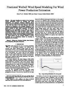
The energy available in the wind varies as the cube of the wind speed, thus, an understanding of the nature of the wind resource is important to all aspects of wind energy exploitation, from the identification of appropriate sites and predictions of the economic viability of wind farm projects through to the design of wind turbines themselves, and understanding their effect on electrical energy distribution networks and consumers. From the point of view of wind energy, the most prominent characteristic of the wind resource is its variability. The wind is highly variable, both geographically and temporally. Moreover, this variability persists over a very wide range of scales, together in space and time. The importance of this is amplified by the cubic relationship to available energy. On a large scale, spatial variability explains the fact that there are several different climatic regions in the world, some much windier than others. These regions are mainly governed by the latitude, which have an effect on the quantity of insolation. In the same climatic region, there is a lot of variation on a smaller scale, principally determined by physical geography - the proportion of sea and land, the size of land masses, and the presence of mountains or plains for instance. The type of vegetation may also have an important influence through its effects on the absorption or reflection of solar radiation, affecting surface temperatures, and on humidity. In the local scale, the topography has the most important effect on the wind nature. More wind could be found on the tops of mountains and hills than in the lee of high ground or in sheltered valleys, for instance. In addition, wind velocities are considerably decreased by obstacles such as buildings or trees. For a given location, temporal changeability on a large scale indicates that the amount of wind may vary from one year to the next, with even larger scale variations over periods of decades or more. These long-term variations are not well understood, and may make it difficult to have correct predictions of the economic viability of particular wind-farm projects. In time-scales less than a year, seasonal wind variations are much more predictable, even if there are large variations on smaller time-scales still, which could be logically understood, are often not easy to predict more than a few days ahead. These "synoptic" variations are associated with the passage of weather systems. Depending on location, there may also be significant variations with the time of day (diurnal variations) which usually can be predictable. On these time-scales, the predictability of the wind is important for integrating large amounts of wind energy into the electrical energy network, to let the other generating plant supplying the network to be organized suitably [32].

10

CHAPTER 2. OVERVIEW OF WIND ENERGY 12

THE WIND RESOURCE

5.0 4.5

Synoptic peak

Spectrum, f.S(f)

4.0 3.5 Turbulent peak

3.0 2.5 Diurnal peak

2.0 1.5 1.0 0.5 0.0

10 days 4 days

24 h 10 h

2 h 1 hr 30 min 10 min 3 min 1 min 30 s

10 s 5 s

Frequency, log (f)

Figure 2.1

Wind Spectrum Farm Brookhaven Based on Work by van der Hoven (1957)

Figure 2.1: Wind spectrum of Brookhaven farm based on work by Van Der Hoventime (1957) of day (diurnal variations) which again are usually fairly predictable. On these time-scales, the predictability of the wind is important for integrating large amounts of wind power into the electricity network, to allow the other generating plant Onsupplying time-scales of minutes down to seconds or less, wind-speed variations the network to be organized appropriately. On turbulence still shorter time-scales minutes down to seconds or less, wind-speed known as can have aofvery considerable effect on the design and pervariations known as turbulence can have a very significant effect on the design and formance of the wind turbine, as well as on the quality of power supplied to the performance of the individual wind turbines, as well as on the quality of power network and its consequence consumers. delivered to the network and on its effect on consumers. der Hoven (1957) a wind-speed spectrum spectrum from longand shortVan derVan Hoven (1957) [33]constructed built a wind-speed from longand short term records at Brookhaven, New York, showing clear peaks corresponding to the term records at Brookhaven, New York, showing clear peaks corresponding to synoptic, diurnal and turbulent effects referred to above (Figure 2.1). Of particular the synoptic, diurnal and turbulent effects referred to above (Figure 2.1) [32]. interest is the so-called ‘spectral gap’ occurring between the diurnal and turbulent peaks, showing that the synoptic and diurnal variations can be treated as quite the Particularly interesting is the so-called "spectral gap" taking place between distinct from the higher-frequency fluctuations of turbulence. There is very littlevariadiurnal and turbulent peaks, illustrating that the synoptic and diurnal energy in the spectrum in the region between 2 h and 10 min.

tions can be considered as quite dissimilar from the higher-frequency fluctuations of turbulence. There is very little energy in the spectrum in the region between and 10 min. Variation in the Wind Resource 2.22 hGeographical

Ultimately the winds are driven almost entirely by the sun’s energy, causing differential surface heating. The heating is most intense on land masses closer to the equator, and obviously the greatest heating occurs in the daytime, which means that the region of greatest heating moves around the earth’s surface as it spins on its axis. Warm air rises and circulates in the atmosphere to sink back to the surface in cooler areas. The resulting motion of the air is influenced by causing coriolis forces due to The winds arelarge-scale driven almost wholly bystrongly the sun’s energy, differences on the earth’s rotation. The result is a large-scale global circulation pattern. Certain surface temperatures. The heating is most intense on land masses nearer to the

2.5

Geographical variations in the wind resource

equator, and evidently the maximum temperatures occur in the daytime, which indicates that the hottest region moves around the earth’s surface as it spins on its axis. Warm air climbs and circulates in the atmosphere to descend back to the surface in cooler areas. The resulting large-scale movement of the air is


11

strongly influenced by coriolis forces 1 caused by the earth’s rotation. The result is a large-scale global circulation pattern. Certain identifiable features of this are well known such as the trade winds2 . The earth’s surface non-uniformity, with its topography of oceans and land masses, ensures that this global circulation pattern is disturbed by smaller-scale variations on continental scales. These variations act together in a very composite and nonlinear manner to produce a slightly chaotic result, which is the origin of the day-to-day prediction difficulty of the weather in some particular places. It is clear that, underlying tendencies are the main reason of clear climatic differences between regions. These differences are adjusted by additional local thermal and topographical effects. Increased wind speed in local regions is due mainly to hills and mountains. This is in part a consequence of altitude - the earth’s boundary layer means that wind speed usually increases with altitude above land, and hill tops and mountain peaks may "project" into the higher wind-speed layers. It is also to a certain extent the effect of the acceleration of the wind flow over and around hills and mountains, and funnelling through passes or along valleys aligned with the flow. Similarly, topography may produce areas of reduced wind speed, such as sheltered valleys, areas in the lee of a mountain ridge or where the flow patterns result in stagnation points. Considerable local variations can be a result of thermal effects. Coastal areas are often windy for the reason of differential temperatures between sea and land. Though the sea is warmer than the land, surface air flows from the land to the sea developing a local circulation, with warm air growing from the sea and cool air sinking over the land. After the land is warmer the pattern reverses. The land will heat up and cool down more rapidly than the sea surface, and so this pattern of land and sea breezes tends to reverse over a 24 h cycle. These properties were important in the early development of wind energy in California, where an oceanic current transports cold water to the coast, near desert regions which heat up powerfully by day. An intervening mountain range funnels the resulting air flow through its passes, generating locally very strong and reliable winds (which are well linked with peaks in the local electricity demand caused by air-conditioning loads). Differences in altitude may also cause thermal effects. Therefore, cold air from high mountains can go down to the plains below, causing quite strong and highly stratified "downslope" winds [32]. 1 An

apparent force that as a result of the earth’s rotation deflects moving objects (as projectiles or air currents) to the right in the northern hemisphere and to the left in the southern hemisphere. 2 any wind that blows in one regular course, or continually in the same direction.

12


2.6

Long-term wind speed variations

It is confirmed that the wind speed at any particular place may be subject to very slow long-term variations. Though the availability of precise historical records is a limitation, careful analysis has demonstrated clear trends. Clearly these may be related to long-term temperature variations for which there is sufficient historical evidence. There is also much debate at the present time about the probable effects of global warming, caused by human activity, on climate, and this will certainly affect wind climates in the coming decades. Despite these long-term tendencies, there may be considerable changes in windiness at a certain location from year to year. These changes have various causes. For instance, they may be due to global climate phenomena such as el nino 3 , changes in airborne particles coming from volcanic eruptions, and sunspot activity. These changes affect considerably the effectiveness of predicting the energy output of a wind farm at a particular location during its expected lifetime [32].

2.7

Annual and seasonal variations

Despite the fact that year-to-year variation in annual mean wind speeds stays difficult to predict, wind speed variations during the year can be well described in terms of a probability distribution. It has been found that the Weibull distribution can give a good illustration of the mean hourly variation of wind speed for the period of a year at several typical locations. It is represented by the following form [32] U F(U ) = 1 − exp − c

k !

(2.1)

where F(U ) is the fraction of time where the hourly mean wind speed exceeds U . It is described by two parameters, a "scale parameter" c and a "shape parameter" k which express the variability about the mean. c is connected to the annual mean wind speed U via the next relationship 1 U = cΓ 1 + (2.2) k where Γ is the complete gamma function. This can be derived by consideration of the probability density function 3 An

invasion of warm water into the surface of the Pacific Ocean off the coast of Peru and Ecuador every four to seven years that causes changes in local and regional climate, associated with a positive anomaly.

13


k ! dF(U ) U k−1 U = k k exp − f (U ) = dU c c

(2.3)

while the mean wind speed is given by Z∞ U= U f (U )dU

(2.4)

0

A special case of the Weibull distribution is the Rayleigh distribution, with ANNUAL ANDis SEASONAL VARIATIONS k = 2, which in fact a reasonably typical value for many locations. In this case,15 √ the factor (1 + 1/k) has the value π/2 = 0.8862. A superior value of k, such pffiffiffi as 2.5 or 3,has point a site where variation of hourly ˆ(1 þ 1=k) thetovalue ð=2 ¼ the 0:8862. A higher valuemean of k, wind such speed as 2.5 with or 3, indicates site themean variation of hourly speed aboutwind the annual referenceato thewhere annual is small, whichmean is the wind case of the trade belts mean is small, as is sometimes the case in the trade wind belts for instance. A lower for example. An inferior value of k, such as 1.5 or 1.2, indicates larger variability value k, mean. such asSome 1.5 or 1.2, indicates greater variability about A few aboutofthe examples are represented in Figure 2.2 the [32].mean. The value examples are shown in Figure 2.2. The value of ˆ(1 þ 1=k) varies little, between of (1 + 1/k) varies little, between about 1.0 and 0.885 see Figure 2.3 [32]. about 1.0 and 0.885 see (Figure 2.3). k=

1.25

1.5

2.0

2.5

3.0

Probability density

0.15

0.1

0.05

0 0

5

10

15

20

25

Wind speed (m/s)

Figure 2.2 Example Weibull Distributions

Figure 2.2: Example of Weibull Distributions 1.00

The Weibull distribution of hourly mean wind speeds during the year is visibly 0.98the consequence of a significant amount of random variation. Nevertheless, there exists also a strong underlying seasonal component to these variations, as a 0.96 result of the changes in insolation during the year driven by the incline of the axis of rotation. 0.94

0.92

0.90

0 0

5

10

15

20

25

14

CHAPTER 2. OVERVIEW OF WINDWind ENERGY speed (m/s) Figure 2.2 Example Weibull Distributions 1.00

0.98

0.96

0.94

0.92

0.90

0.88 1.0

1.2

1.4

1.6

1.8

Figure 2.3

2.0 2.2 Shape factor, k

2.4

2.6

2.8

3.0

The Factor ˆ(1 þ 1=k)

Figure 2.3: The Factor Γ (1 + 1/k) Therefore, in moderate latitudes, the months of winter have a tendency to be considerably windier than the months of summer. There may also be a tendency for powerful winds or gales to develop during spring and autumn equinox’s times 4 . Tropical regions also know seasonal phenomena such as tropical storms and monsoons5 which have an impact on the wind climate. Certainly the extreme winds coupled with tropical storms may considerably influence the design of wind turbines intended to subsist in these sites. Even if a Weibull distribution represents a good illustration of the wind regime at many locations, it is not always true. for instance, some sites presenting clearly diverse wind climates in summer and winter can be characterized better by a double-peaked ’bi-Weibull’ distribution, with dissimilar scale factors and shape factors in the two seasons, i.e. [32],   !  !   U k1   U k2   + (1 − F1 ) exp −  F(U ) = F1 exp −  c  c1  2

2.8

(2.5)

Synoptic and diurnal variations

Wind speed variations are to some extent more random on shorter time-scales than the seasonal changes, and more difficult to predict. On the other hand 4 The

time or date (twice each year, about 22 September and 20 March) at which the sun crosses the celestial equator, when day and night are of equal length. 5 The monsoon is the season in Southern Asia when there is a lot of very heavy rain.


15

these variations enclose definite patterns. The frequency signal of these variations generally peaks at about 4 days or so. These are called synoptic variations, which are linked with large-scale weather patterns such as regions of low and high pressure and associated weather fronts as they move across the earth’s surface. Coriolis forces provoke a circular movement of the air when moving from high- to low-pressure regions. These coherent large-scale atmospheric circulation patterns may normally take a few days to pass over a given point, even if they may occasionally "stick" in one position for longer before moving on or dissipating in the end. In the frequency spectrum of higher frequencies, many locations will demonstrate different diurnal peak at a frequency of 24 h, which is usually caused by local thermal effects. Strong heating in the daytime can cause large convection cells in the atmosphere, which die down at night [32].

2.9

Components of wind energy systems

A wind turbine is a core device of a wind energy system; it converts the wind power into electricity energy. This is contrary to a "windmill", which is a machine that converts the wind’s power into mechanical power. The same as electricity generators, wind turbines are linked to some electrical network. These networks comprise battery charging circuits, housing scale power systems, isolated or island networks, and large utility grids. In terms of total numbers, the most commonly found wind turbines are in fact quite small - on the order of 10 kW or less. In terms of total generating capacity, the turbines that constitute the majority of the capacity are usually quite large - in the range of 500 kW to 2 MW. These big turbines are employed mainly in large utility grids, principally in Europe and the United States. A representative modern wind turbine, linked to a utility network, is shown in Figure 2.4. These basic components consist of [34]: • A rotor: which is a set of blades with aerodynamic surfaces. When the wind touches the blades, the rotor turns, and hence the generator or alternator in the turbine turn and generate electricity; • A gearbox: which matches the rotor speed to the generator/alternator speed; • An enclosure, or nacelle, used to protect the gearbox, generator and other turbine components from the elements; • A tailvane or yaw system, which lines up the turbine with the wind.

16


Gearbox

Rotor with blades

Generator Alternator

Tailvan

Circuit Breaker

DC to AC Inverter

Nacelle

Optional System Equipment

Battery Disconnect Switch

Batteries

Turbine Disconnect Switch Tower

Figure 2.4: Components of a wind energy system To understand how wind turbines are employed, it is helpful to concisely consider a number of the elementary facts underlying their operation. In present wind turbines, the actual conversion process utilizes the basic aerodynamic force of lift to create a net positive torque on a rotating shaft, resulting first in the creation of mechanical power and after that in its transformation to electricity in a generator. Wind turbines, dissimilar from the other generators, can generate energy only in response to the wind that is directly available. It is impossible to store the wind and exploit it a later time. The output of a wind turbine is therefore naturally fluctuating and non-dispatchable. Any system to which a wind turbine is linked must somehow take into account this variability. In the large networks, the wind turbine helps to decrease the entire electrical load and consequently results in a decrease in either the number of usual generators or in the fuel used of the running generators. In the small networks, we may find energy storage, backup generators, and some specific control systems. Other interesting property is that the wind is not transportable: it can just be converted where it is blowing. Nowadays, the possibility of transmission electrical energy by means of power lines compensates for wind’s incapability to be transported [35].

17


2.9.1

Modern wind turbine design

At present, the most common design of wind turbine is the horizontal axis wind turbine (HAWT). Where, the rotation axis is parallel to the ground. HAWT rotors are generally classified according to the rotor orientation (upwind or downwind of the tower), hub design (rigid or teetering), rotor control (pitch vs. stall), number of blades (generally two or thee blades), and how they are aligned with the wind (free yaw or active yaw). Figure 2.5 illustrates the upwind and downwind configurations [34]. Wind Direction

Upwind

Wind Direction

Downwind

Figure 2.5: HAWT rotor configurations

2.10

Historical utilization of wind power

For many centuries, the wind has been utilized to power sailing ships. A lot of countries owed their prosperity to their sailing skill. The New World was discovered via wind powered ships. In fact, wind was almost the single source of power for ships until Watt invented the steam engine in the 18th Century [34]. On land, wind turbines date back many centuries. In the seventeenth century B.C, the Babylonian emperor Hammurabi have been planned to utilize wind turbines for irrigation. Hero of Alexandria, who lived in the third century B.C., has given a description to a four sails wind turbine with simple horizontal axis which was used to blow an organ. The Persians were using wind turbines widely by the middle of the seventh century. There was a vertical axis machine with a number of sails mounted radially [4].


18

These former devices were certainly basic and mechanically ineffective; however they served their purpose well for a long time. They were made from local resources by cheap labour. Maintenance was possibly a difficulty which served to keep many people at work. Their size was probably dictated by the accessible materials. A need for additional power was satisfied by constructing further wind turbines rather than larger ones. There are several smaller countries of the world today which can usefully utilize such low technology machines due to the large amounts of cheap, inexperienced labour available. Such countries often have difficulty obtaining the foreign exchange needed to acquire high technology equipments, and then have complexity maintaining them. The former English wind turbine date to 1191. The first corn-grinding wind turbine was constructed in Holland in 1439. There were a few technological improvements throughout the centuries, and by 1600 the most widespread wind turbine was the tower mill. The word mill refers to the action of milling or grinding grain. This application was so usual that all wind turbines were often called windmills even when they pumped water or carried out some other operation. The tower mill had a fixed supporting tower with a rotating cap holding the wind rotor. The tower was generally built of brick in a cylindrical form, and sometimes was built of wood, with polygonal cross section. In one manner, the cap had a support or tail extending out and down to land level. The tower was surrounded by a circle of posts where the support touched the soil. The miller have to check the direction of the dominant wind and turn the cap and rotor into the wind with a winch connected between the tail and one of the posts. The tail is then attached to a post to maintain the rotor in the right direction. This operation would be repeated after the wind direction changed. Protection from high winds was implemented by turning the rotor out of the wind or taking out the canvas wrapping the rotor latticework. The development of the rotor form perhaps took a long time to complete. It is worth noting that the rotors on the majority of the Dutch mills are twisted and tapered to get a maximum efficiency. The rotors at the moment on the tower mills possibly do not get reference from the original structure of the tower, but still reveal a high quality aerodynamic engineering of an earlier period. In the mid-1700’s, Dutch colonist bring this kind of wind turbine to America. A number were constructed, but not the same number which was in Europe. Then in the mid-1800’s, a need expressed for a small wind turbine to pump water. The American West was being colonized and there were wide zones of good grazing lands with no surface water but with generous ground water just a few

meters beneath the ground. In such conditions, a typical wind turbine was constructed, named the American Multi-bladed wind turbine. It had high starting torque and satisfactory efficiency, and fulfilled the wanted water pumping purpose very well. If there is no wind activity for several days, the pump would be activated by hand. Because this is a rationally good wind regime, hand pumping was relatively rare to happen. Between 1880 and 1930, an approximate 6.5 million units were constructed in the United States by several companies, a lot of are still working satisfactorily. By supplying water for livestock, these machines played an important role in settling the American West [4].

2.11

Conclusion

As wind power is a renewable energy, it is considered as a better option in preference to the conventional energy resources like fossil fuels. In this chapter, it is introduced the most important principles and concepts related to the wind energy, its nature, origin and the main constituents related to a good understanding of its characteristics. To comprehend how to convert the wind into electrical power, a brief introduction to wind turbine technology is provided. Finally the historical use of wind energy is reported in the last section.

CHAPTER

3 WIND FORECASTING: LITERATURE REVIEW


21

3.2 Time-scale classification . . . . . . . . . . . . . . . . . . . . . .

21

3.3 Synopsis of wind forecasting methods . . . . . . . . . . . . . .

21

3.3.1

Persistence method . . . . . . . . . . . . . . . . . . . . .

22

3.3.2

Physical approach . . . . . . . . . . . . . . . . . . . . . .

22

3.3.3

Statistical approach . . . . . . . . . . . . . . . . . . . . .

24

3.3.4

Hybrid approach . . . . . . . . . . . . . . . . . . . . . .

25

3.4 Wind speed against wind power . . . . . . . . . . . . . . . . .

25

3.5 Review of wind forecasting techniques . . . . . . . . . . . . .

26

3.6

3.5.1

Very-short term forecasting . . . . . . . . . . . . . . . .

26

3.5.2

Short term forecasting . . . . . . . . . . . . . . . . . . .

27

3.5.3

Medium term forecasting . . . . . . . . . . . . . . . . .

29

3.5.4

Long term forecasting . . . . . . . . . . . . . . . . . . .

31

Conclusion . . . . . . . . . . . . . . . . . . . . . . . . . . . . .

33

20

CHAPTER 3. WIND FORECASTING: LITERATURE REVIEW

3.1

21

Introduction

Improved wind-forecasting is considered as an efficient means to overcome many of the energy market’s difficulties. For instance, regarding competitive electricity markets, precise wind forecast is always appealing for a variety of reasons. Firstly, appropriate incentives of attractive market price are offered on energy imbalance charges based on market price. Secondly, a correct forecast can help to develop well-functioning hour-ahead or day-ahead markets [5, 8]. Many of the stated topics are further discussed in [36–39]. A probabilistic method for estimating energy expenses associated with prediction errors for wind generators is discussed in [36] where case studies demonstrate that error prediction costs can attain up to 10% of the entire revenues from selling wind power. A short term probabilistic forecast of wind power is discussed in [37] where it is presented a method for optimal bidding strategy derived from uncertainty information of forecasts. Some good reviews on wind speed prediction and power generation could be found in the literature [40–42]. In this chapter, a large overview of wind prediction techniques is provided with respect to both: i) prediction technique category and ii) prediction time horizon. Covering the majority of wind speed techniques found in the literature.

3.2

Time-scale classification

Time-scale classification of wind forecasting methods is vague. However, as shown in Table 3.1 [6], wind forecasting can be classified into four categories: • Very short-term forecasting: From few seconds to 30 minutes ahead; • Short-term forecasting: From 30 minutes to 6 hours ahead; • Medium-term forecasting: From 6 hours to 1 day ahead; • Long-term forecasting: From 1 day to 1 week ahead.

3.3

Synopsis of wind forecasting methods

A general summary of wind forecasting methods is reported in Table 3.2 [6]. The majority of wind forecasting techniques developed and presented in literature use one of the followings:


22

Table 3.1: The applications of specific time horizon with respect to the function of electricity systems. Time horizon Range Applications Very short term Few seconds to - Electricity market clearing 30 minutes ahead - Regulation actions Short-term 30 minutes to - Economic load dispatch planning 6 hours ahead - Load increment/decrement decisions Medium-term 6 hours to - Generator online/offline decisions 1 day ahead - Operational security in day-ahead electricity market Long-term 1 day to 1 week - Unit commitment decisions or more ahead - Reserve requirement decisions - Maintenance scheduling to obtain optimal operating cost

3.3.1

Persistence method

This method is also called "Naïve Predictor". It is supposed that the wind speed at time t + ∆t will be equal as it was at time t. Incredibly, it is more accurate for very-short to short term forecasts than the majority of the physical and statistical methods. It is still used by industry for very-short term forecasts [5], [43]. For this reason, any developed forecasting method have to, first, be compared against the traditional persistence method to verify how much it can improve over this technique [44].

3.3.2

Physical approach

Physical systems use parameterizations derived from an entire physical description of the atmosphere. Generally, wind speed provided by the weather agency on a coarse grid is transformed to the onsite conditions at the wind farm site [45].

3.3.2.1

Numeric Weather Prediction (NWP):

This method is classified as a physical approach to wind forecasting. NWP models work by solving complex mathematical models that utilize weather data such temperature, pressure, surface roughness and obstacles. NWPs are operated on supercomputers since they require lots of computations. Usually, NWPs are run 1 or 2 times a day because of the complexity to gain information in short-time and the related high costs. This limits its effectiveness to medium to long-term


23

Table 3.2: Basic wind speed and power forecasting methods Forecasting Method Persistence Method/ Naïve Predictor

Subclass –

Examples P (t + k) = P (t)

Physical Approach

Numeric Weather Predictor (NWP)

Statistical Approaches

Artificial Neural

- Global Forecasting System - MM5 - Prediktor - HIRLAM, etc. - Feed-forward - Recurrent

Networks

- Multilayer Perceptron

(ANN)

- Radial Basis Function - ADALINE, etc - ARX - ARMA - ARIMA - Grey Predictors - Linear Predictions - Exponential Smoothing, etc. - Spatial Correlation

Timeseries models

Novel Techniques

–

- Fuzzy Logic - Wavelet Transform

Hybrid Structures

–

- Ensemble Predictions - Entropy based training, etc. NWP+ANN - ANN + Fuzzy logic = ANFIS - Spatial Correlation + ANN - NWP+time series

Remarks - Benchmark approach - Very accurate for very short and short term - Use of meteorological data such as wind speed and direction, pressure, temperature, humidity, terrain structure etc. - Proved better for long term. - Proved better for short-term - Their hybrid structures practical for medium to long term forecasts - generally, outperform time series models

- Proved better for short-term - Some very good Time series models replace ANN structures.

- Spatial correlation is good for short term. - Entropy based training of model improves the model performance. - non-Gaussian error pdf improves the model accuracy - ANFIS more accurate for veryshort term forecast. -NWP + ANN models are very accurate for medium and longterm forecasts.


24

forecasts (> 6 h ahead). These methods present a better precise predictions when weather conditions are stable [43, 46].

3.3.3

Statistical approach

The statistical approach is based on learning a model with historical experimental data and uses difference between the actual and the predicted wind speed values to adjust model parameters [43, 45]. It is straightforward to model, inexpensive, and provides timely predictions. It is not based on any predefined analytical model and rather it is based on patterns. The error minimization is achieved by fitting the patterns to the historical data. Sub-classification of this approach is: Time-series based models, and artificial neural network (ANN) based methods. Auto-Regressive models (AR) are the most popular kind in the time-series based approach to predict future values of wind speed or power. A number of varieties are autoregressive models, moving average model (MA), autoregressive moving average model (ARMA) [12], autoregressive integrated moving average model (ARIMA) [13, 14]. The Neural Networks are trained using past data taken over a long timeframe to learn the relationship between input data and output wind-speeds. In general, ANNs have an input layer where historical data are fed for learning, one or more hidden layer(s) and an output layer providing prediction values [18,19]. (They include: Multi-Layer Perceptrons (MLP) [20, 21], Radial Basis Functions Networks [22](RBFN) and Recurrent Neural Networks (RNN) [23, 24]), Fuzzy Logic [25], and Support Vector Machines (SVM) [26, 27]. In general, ANNs perform better than time-series models for approximately all time-scales, even if this is not necessarily general. For instance, s-ARIMA (Seasonal ARIMA) and Adaline ANN models are applied to predict wind speed in Mexico and are compared with each other [47]. The results confirm that sARIMA fit better the actual pattern. Likewise in [48], the single exponential smoothing model is applied for forecasting. The later follows very well the actual trend with a good values of error adjustment coefficient. The Comparison with the Adaline ANN demonstrates that exponential smoothing model reveals better sensitivity to the tuning and prediction of the wind speed. However, when the number of the input training vectors is increased for the given ANN model, its performance gets improved.


3.3.4

25

Hybrid approach

In general, combination of diverse methods such as combining statistical and physical models or mixing short term and medium-term models, and so on, is called a hybrid approach. For example, radiative transfer and ANN approaches are combined with Special Sensor Microwave/Imager (SSM/I) to obtain the wind speeds and direction of ocean surface in [49]. Results illustrate that combination of ANN can significantly improve the effect of these data in NWPs than just using SSM/I. Among the recent techniques is the model derived from the spatial correlation of wind speeds, where a spatial relation between wind speeds at different locations is considered. The historical wind time-series of a considered site and its neighbouring sites are used to forecast the future wind speed value, generally by ANNs or adaptive neuro-fuzzy networks [25, 50]. This is due to the fact that changes in wind speed time-series remote stations will be observed at local station with some time delay.

3.4

Wind speed against wind power

Power production of a wind turbine is directly related to the wind speed, which varies with time and depends on regional weather conditions and type of landscape. Relationship between wind speed v(m/s) through swept area A(m2 ) of wind turbine and wind energy per unit time or wind power P (W ) is [32] 1 P = ρAv 3 (3.1) 2 where ρ is the density of air (kg/m3 ), which is based on pressure and temperature of air. From this relationship, it is clear that the relationship between wind speed and power is nonlinear, essentially cubic. Accordingly, any error incurred in wind speed forecast will cause a large cubic error in wind power. Additionally, for the complete wind farm, this relation is more complex because different turbines in the farm use various wind directions and speeds to get optimal power output of wind farm. Hence, small error in wind speed forecast can produce a large error in wind power forecast. To convert wind speed into power, it is recommended to use the producer’s power curve for each wind turbine independently and combine the results; as in [51–54]. But this will not give an optimal result. Thus, as illustrated in [5], the improved approach is to use a power curve


26

formed using recorded wind speed values at the location. This is able to improve Root Mean Squared Error (RMSE) of forecast by about 20% compared to when manufacturer’s power curve used.

3.5

Review of wind forecasting techniques

Based on the timescales, this present section is divided into four parts. For each timescale, different forecasting techniques reported recently in the literature are discussed in brief as below.

3.5.1

Very-short term forecasting

Only a few papers are presented for very-short term forecasting timeframe. A case study from Tasmania, Australia for very short-term (2.5 minutes ahead) forecasting using "Adaptive Neuro-Fuzzy Interface System" (ANFIS) to forecast wind vectors is proposed in [43], it is reported that wind direction could have great impact to obtain a better forecasting precision over very-short term timescale. To build the model, dataset containing 21 months time series in steps of 2.5 minutes is used, wind speed and direction are projected into two vectors ’u’ and ’v’. The results confirm that ANFIS gave less than 4% mean absolute percentage error (MAPE) while that for persistence is about 30% in deciding either ’u’ or ’v’. It is also recommend developing very-short term forecast models for time duration a little longer, since several deregulated markets are cleared every 5 minutes and settlements are done each 30 minutes. This is described in [8] for the timeframe of 5 to 15 minutes. Tests are done with actual wind speed data of 30s resolution from a wind farm. It is recommended, to develop a system that forecasts for 30 min timeframe for future research, and to consider the conditions like non-uniform wind speeds in a single park. A combination method based on ’linear prediction model’ of ARMA with ’filtering’ of wind waveforms for wind speed forecasting is reported in [17]. A linear combination of actual and past samples is given as output. Wind speed signal is passed by a low pass filter of the wind turbine mechanical system, since the spectrum of a signal with small frequency components exposes better short term prediction, Prediction results of 1s and 5s ahead are reported in [55].


3.5.2

27

Short term forecasting

The majority of research on wind forecasting has been done in this time scale. Short-term forecasting of 1-h ahead is discussed in [56] where the authors propose an AR model of 6th order based on Bayesian approach. Comparison with persistence model indicates efficiency of method although lower order AR models fail to give satisfactory accuracy. ARMA with historical data for 6-h advance predictions is reported in [44]. The reported approach outperforms persistence by 7% in the first hour and 18% in the sixth hour. The test results of the model for 10-min ahead timescale provide poor performance illustrating that the capability of ARMA models changes when applied to different time periods. Using a case-study of a Mexican wind farm, a hybrid model combining nine different statistical forecasting methods is investigated in [55]. The final prediction is achieved by an aggregated single model using adaptive linear combination of alternative methods, where the weight of every model is derived from its actual forecast performance. Results demonstrate that final forecast of power is almost identical to its real values. Auto Regressive Model with External Inputs (ARX) and ANN models versus persistence method for the forecasting horizons of 1, 3, 6 and 12 hours are compared in [57]. Tests show that persistence is better than ARX for horizons lesser than 13 hours; whereas ANN model outperforms persistence model. In [23], RNNs are employed for scheduling autonomous wind-diesel system for a horizon of 2 hours. Three diverse ANN architectures are assessed with RMSE criterion. All the architectures outperform the persistence model. A Mexican case study using ANN to the hourly prediction of time series is discussed in [58]. For each month of year, a model is developed. Four dissimilar ANN architectures are assessed. The simplest architecture with two layers, two input neurons and one output neuron proved to be the best with 0.0016 Mean Square Error (MSE) and 0.0399 Mean Absolute Error (MAE) values. Examples of [23] and [58] clarify that the choice of an appropriate ANN architecture necessitates careful examination and depends on the problem description. Under the framework of kernel-machines, a Gaussian Process (GP) with Bayesian estimation for predicting lower and upper limits and average of wind speed 1-hour horizon is presented in [59]. Historical wind speed data in addition to other meteorological features are tested with GP and evaluated against RBFN and MLP ANN models. GP experimental results show an improvement of 27% of average error and 13% of maximum error.


28

Spatial correlations for 15-min to 3-hour ahead speed forecasting using ANNs for predicting the relation between recorded data at 1 reference and 2 remote sites are employed in [50]. Inputs are 1 to 5-min wind speed averages from remote sites. Using two cases of long and short spatial distances, results show that forecasting effectiveness was enhanced by 28% against the persistence, suggesting that data from neighbouring sites are always valuable. A further application of spatial correlation method using Takagi-SugenoKang (TSK) fuzzy interface model for 2-hour ahead forecasting is proposed in [25]. Inputs are wind speeds given by "upwind station". The model training was carried out by means of genetic algorithm. Case results of ’flat terrain’ presents an improvement of 29% over naïve predictor, while in the case of "complex terrain", the model proved non successful because of the non-correlation between local and remote sites. In [18], three different architectures of ANNs specifically BP, adaptive linear element, and RBFN for 1-hour ahead wind speed prediction are discussed, the error assessment is done with three different error criteria MAE, RMSE and MAPE. Experimental tests were carried out by varying the number of wind features given to the ANN input with diverse learning rates. For each ANN model, experimental results show that different optimal architectures were found for each different site and error criterion; i.e., none of ANNs outperform others universally. This recommends that the configuration of ANN model to be utilized, number of model inputs and learning rates have to be carefully chosen. A universal evaluation criteria and robust method are required for combining predictions from different models. A novel approach called Mycielski was introduced in [60]. Where, next value in the current random process is the longest repeating data chain that has been recorded in the historical data sequence. The methodology validation was carried out on three Turkish case studies; presenting a maximum RMSE of only 1.5%. The model proved robust; therefore the authors recommend the model to be employed for forecasting in any region. In [61], first, data were pre-processed to extract properties such standard deviation, average and slope prior to providing it to either ANN or fuzzy logic. This diminishes the fuzzy rule base or ANN size and make more fast the learning process. For the presented approach, RMSE and coefficient of determination (COD) used as evaluation criteria gave less computational time, less RMSE and more COD.


29

A new 1-hour ahead forecasting method derived from Grey model (GM) is proposed in [62], where the original time series data are transformed into a new series with less noise and randomness. Next, a differential equation is formed with a coefficients computed by means of least square method. Predicted values of new series are computed with these coefficients, and actual forecasted values of original series are restored using inverse operation. However, it presents overshoots and therefore, to reduce them, alpha GM is proposed in [63], it is based on weighting factors for calculating differential equation coefficients. However, it has poor time-series tracking feature. To this end, two new models "Improved GM" and "Averaged GM" have been proposed. Improved GM generates two shifted-prediction models from the normal GM. Next, the two models are combined to make final improved GM based on their weights. In averaged GM, the weights are the same for both models (i.e., 0.5 for each one). Experimental results with MAE and RMSE error criteria show that all models outperform the standard persistence model. Additionally, average GM has a general superiority over all GMs and naïve predictor. A hybrid approach is presented in [51]. It uses wavelet technique to decompose the original time-series data into a number of subseries. Next, an improved ARIMA method is applied to forecast the future values in each subseries. Results of subseries are then combined and compared with standard time-series model and BP ANN with MAE, MSE and MAPE criteria. The proposed method offers enhanced results (less error) compared to others for 3-step, 5-step and 10-step ahead prediction respectively. It is concluded that, a better accuracy is achieved for smaller forecasting steps and vice versa. In [52], it is proposed an "augmented complex statistics" based linear sequential least mean square algorithm (ACLMS), for instantaneous modelling of wind speed and direction in the complex numbers domain. The prediction of wind power is done by finite impulse response (FIR) filter. Results are assessed against "standard complex filter" for wind data sampled with a small interval over 1-, 3- and 6-hour intervals with MAE and COD criteria, it presents an important improvement for ACLMS algorithm.

3.5.3

Medium term forecasting

The majority of methods proposed for this time-scale are based on ANN techniques, physical weather models, and hybrid models combining these models or some recent techniques. In [64], wavelet transform is used to decompose the original signal and divide data into several subsets with different frequency components. The coefficients of decomposed waveforms are estimated by a pre-


30

diction technique, which are then reconstructed to obtain the original samples together with forecast of next 24 hours. Experimental assessment with MSE shows that only one or two out of four different daubechies wavelets do better than persistence method. A case-study by means of Feedforward Neural Networks (FNN) trained using Levenberg-Marquardt (LM) algorithm is proposed in [65] for 1 to 24-hour ahead forecasts. Optimal number of neurons was obtained experimentally by an error method. A MAPE improvement of 12% for FNN compared to persistence method with a computational time of 5s only. A hybrid approach for 1 to 48-hour ahead forecasts is presented in [52]. It offers preliminary forecast based on NWPs using RBFN. The evaluation of the quality of forecast was accomplished by calculating the errors between the estimated and actual values of power and direction. The "poor" NWPs were enhanced by fuzzy rules to get better predictions. Results comparison is based on MAE and RMSE in opposition to naïve predictor and ’just’ NWP method; presenting a significant improvement for both (up to 46%). Also, a comparison of the proposed model with the state of the art statistical model, with NWPs’ and online-prediction data as input is proposed in [66]. Results show that hybrid approach of [52] outperforms the state-of-the-art method. A special case of ARIMA process is proposed in [67]. f-ARIMA model parameters were computed using "exact maximum likelihood" optimized according to the Akaike’s Information Criterion, which evaluates the accuracy versus the complexity of the model. Results with COD, Daily Mean Error (DME), and variance presented a very high COD (95%) and very low DME and variance in comparison with the standard persistence and ARIMA models. Projection from wind speed to wind power forecasts also presents accurate results for 24 to 48hour ahead. In [68], it is proposed to evaluate the performance of a regional NWP, called Eta model. Eta forecasts 12 to 36-hour ahead wind speed forecasts are evaluated against wind recorded at nearest surface station at the elevation of 10 m in Sweden. The results present a high COD (0.8), and low MAE and RMSE. Consequently, Eta model is recommended for wind energy prediction. A two-stage hybrid model is proposed in [69]. A "Bayesian clustering by dynamics" classifies the input training dataset into a number of subsets with similar properties in unsupervised mode. A ’support vector regression’ learns the training data in each subset in a supervised manner. Past wind generation behaviour is extrapolated by finding hidden recurring trends, structural


31

changes etc. using RQA analysis for 1 to 48-hour ahead forecasts. Based on RMSE and MAE error criteria, the proposed methodology outperforms the persistent model for all predictions by around 40%. In [70], the standard hypothesis of Gaussian distribution of wind power forecast error is discussed by analyzing the errors against persistence for 1 to 24-hour ahead forecast, demonstrating that their kurtosis varies from 3 to 10, corresponding to Beta probability distribution function (pdf); whereas that of Gaussian distribution is equal to 3. To confirm this, forecast results are arranged into several power bins and pdf within each bin is roughly the Beta pdf. Results for a 24-hour ahead forecast show that Beta pdf fits in a perfect manner the actual data. A case-study for sizing an "Energy Storage System" shows that the presented model performs very well for loss values larger than 2%.

3.5.4

Long term forecasting

As mentioned earlier, long-term forecasting is very important in restructured electricity markets and its applications. A new kind of physical method for the estimation of wind power generation for 1-to-10 days ahead forecast by means of "weather ensemble predictions" (WEP) is proposed in [71]. The model is calibrated and smoothened to suitably predict the uncertainty in weather conditions. Comparison of results over a period of week with classical time series methods (ARMA based models) shows that WEP presents more precise predictions. In [72], numerical wind speed and direction forecasts are fed as input to three RNNs for timescale prediction of 72-hour ahead. The results comparison of two FNNs and the naïve predictor based on MAE and RMSE criteria, show that RNNs outperform persistence by around 50% and follow the real power curve more narrowly than FNNs. It is remarked that the prediction accuracy improves when additional "nodes" are added. Method of [72] is very exhaustive and time-consuming. Thus, it is necessary for RNN to forecast in smaller times and without involving excessively meteorological data or complications. This is presented in reference [73] by using RNN for wind speed forecasts of each month independently. RNN is trained by 1 year data at only one site. Results indicate that, RNNs presents more accurate results than FNNs for some hours to 1 day-ahead forecasts. Fifth generation mesoscale (MM5) model using meteorological data from a global NWP is proposed in [74]. Ensemble models are developed in order to obtain mean hourly wind speed predictions at Spanish wind farm. These in ad-


32

dition to wind direction and temperature are fed to ANN to obtain wind speed forecasts of 48-hour ahead for each wind turbine. The results assessment is done with MAE and MSE error criteria. In addition, a statistical analysis is carried out in order to prove the superiority of the proposed methodology over the standard ANN approach. Curves of predicted and actual wind speeds illustrate that hybrid system follows the actual wind series very narrowly. In [53], two hybrid systems of MM5 and ANNs are combined in such a manner that ANNs work as transfer functions between NWP wind speed and direction forecasts and corresponding electric power generation; the last measured values of wind power are used to get forecast in the first hours. A system known as FORECAS uses single MLP; while SGP system uses combination of Kalman filter, ARMA model and several ANN models, all optimized with fuzzy system. Simulation results show that FORECAS and SGP present fairly accurate predictions of the wind power with an improvement of 48% on average over persistence model. Several FNN architectures such as 1 or 2 hidden layers, varying number of neurons (5 to 15) and different learning algorithms like "scaled conjugate gradient" and LM for predicting the mean monthly wind speed of 28 sites in Nigeria are explored in [21]. The input variables were latitude, longitude, altitude, and month of year. The optimal architecture was obtained by two hidden layers with 15 neurons for each layer using LM algorithm. The model assessment gave 8.9% of MAPE, and 93.8% COD. The developed model is used to monitor and forecast wind speed at locations with no monitoring stations. For non-Gaussian error distribution, error criteria derived from minimizing information content or entropy such as MEE (minimum error entropy), MCC (maximum correntropy) or MEEF (MEE with fiducial points) instead of minimizing its variance (MSE criterion) are more appropriate to train the forecast models, as proposed in [75]. To confirm this, tests based on MCC and MEEF criteria against MSE criterion were performed on FNNs with one hidden layer containing nine neurons for 3 days-ahead forecasts with half hour sampling. FNNs inputs were wind speed and direction. In the case of offline training, ANNs trained with MEEF and MCC presented a Normalized MAE improvement of 1.5% when compared with ANNs trained according to MSE criterion. For online training, this was approximately 1.15%. The average difference between online and offline trained MEEF was 1.56%. Further improvements can be obtained if this approach is integrated into some more advanced wind power prediction techniques.

3.6

Conclusion

This chapter presented a literature review on forecasting of wind speed and generated power with regard to different time scales. With the intention to provide the reader with a broad understanding of the state of the art methods used in wind speed prediction, numerous forecasting models, which have their own descriptions, were discussed and presented. A number of them are good at short-term prediction whereas others perform better in long-term prediction; some are simple and broadly used while other complex ones have more accurate results. Recently, with the progress of artificial intelligence and mathematical tools, several new methods were suggested. Many of them are more outstanding than the conventional methods and have good development prospect. The most important focus was to give emphasis to the variety of diverse forecasting methods available.

CHAPTER

4 STATIC WIND SPEED PREDICTION


35

4.2 Problem formulation . . . . . . . . . . . . . . . . . . . . . . . .

36

4.3

Prediction process . . . . . . . . . . . . . . . . . . . . . . . . .

36

4.3.1

Multiple linear regression . . . . . . . . . . . . . . . . .

37

4.3.2

Multi-layer perceptron neural networks . . . . . . . . .

37

4.3.3

Radial Basis Functions neural networks . . . . . . . . .

38

4.3.4

Support vector machines . . . . . . . . . . . . . . . . . .

39

4.4 Fusion process . . . . . . . . . . . . . . . . . . . . . . . . . . . .

41

4.4.1

Average Strategy(AS) . . . . . . . . . . . . . . . . . . . .

41

4.4.2

Weighted Strategy (WS) . . . . . . . . . . . . . . . . . .

41

4.4.3

Non-linear Strategy (NLS) . . . . . . . . . . . . . . . . .

42

4.5 Experimental assessment of the MAS . . . . . . . . . . . . . .

42

4.6

4.5.1

Data description . . . . . . . . . . . . . . . . . . . . . . .

42

4.5.2

Single models learning . . . . . . . . . . . . . . . . . . .

44

4.5.3

Experimental results . . . . . . . . . . . . . . . . . . . .

47

4.5.4

Hypothesis testing of the MAS . . . . . . . . . . . . . . .

52

Conclusion . . . . . . . . . . . . . . . . . . . . . . . . . . . . .

54

34

CHAPTER 4. STATIC WIND SPEED PREDICTION

4.1

35

Introduction

A sustainable energy supply, both in the short and the long-term, is needed for promoting both economic development and people’s quality of life, as well as protecting the environment. In this context, wind may be one of the most significant renewable energy sources for the next few decades [32]. New wind power projects have proven that wind energy not only is cost competitive, but also offers additional benefits to the economy and the environment. The development of wind energy carries the economic benefits of creating jobs and new businesses while supporting local economies and reducing reliance on imported energy [76]. Along with the fast growth of wind power generation and the increasing integration of wind power into energy systems, effective techniques and methods of wind speed prediction are becoming more and more important and immediately needed for the characterization and prediction of wind resource as well as for the integration of wind power into energy systems. The MAS proposes to exploit the peculiarities of different prediction algorithms (MLR, ANN and SVM) by means of a Multiple Architecture System [31]. The MAS relies on the idea to fuse the estimates obtained by an ensemble of different prediction techniques, in order to exploit synergistically predictors with different characteristics. If the ensemble is suitably designed, the MAS can result in more accurate and reliable final prediction than those provided by the single prediction algorithms [77]. Note that the proposed approach takes origin from combining classifiers [78], and closely related to the ensemble learning theory [30]. In this chapter, we present the two building stages of the MAS. The first stage consists in training different regression methods for the Input data. For this reason, we will explore both linear (Multiple Linear Regression (MLR) and Linear Support vector Machines) as well as non-linear regression algorithms (the Multi-layer Perceptron Networks, Radial Basis Functions Neural network, Gaussian SVM and Polynomial SVM). In the second stage, the estimates yielded by the ensemble of linear and non-linear predictors are combined in order to make a final estimate of the wind speed. Three combination (fusion) strategies are investigated. The first linear fusion strategy is based on a simple average operation, while the second one carries out a weighted averaging after determining the weights to be assigned to each predictor. The non-linear fusion is accomplished by means of an ANN method. The experimental assessment of the MAS was carried out on the basis of real data set. Finally, a statistical analysis of the MAS based on hypothesis testing is presented.

36


4.2

Problem formulation

Let us consider a set of training samples xi = (i = 1, ..., N ) represented in the ddimensional variable space T ):        f1 (x1 ) f2 (x1 ) ... fT (x1 )   β1   y1   f (x ) f (x ) ... f (x )   β   y   1 2 2 2 T 2    2   2  ¯ β¯ = Y¯ .. ..  ×  ..  =  ..  ⇔ F.  .. . .   .   .   . . . .       yT βT f1 (xN ) f2 (xN ) ... fT (xN )

(4.16)

An interesting property of WS is that, if proper values of the reliability factors are used, the combination of the predictions obtained from the different single predictors is less sensitive to their respective bias and variance than in the AS strategy.

4.4.3

Non-linear Strategy (NLS)

The non-linear strategy can be useful when the outputs of the predictors have a complex relationship that cannot be captured by a simple linear model. Note, that all non-linear predictors presented in this work can be used for this strategy. Accordingly, an MLP network was chosen for such a purpose (see Subsection 4.3.2).

4.5 4.5.1

Experimental assessment of the MAS Data description

There are 7 locations in Algeria where mean daily values of meteorological parameters were measured and recorded. These measured parameters include mean, maximum and minimum values of temperature and mean wind speed. Daily values of wind speed recorded for a period of 10 years (between 1995 - 2004) were used for all 7 locations [101]. Table 4.1 shows names, latitude, longitude, altitude and number of records for each location. As seen from Figure 4.5, these stations cover the four directions of Algeria, from east to west and from north to south, including the central area.


Table 4.1: Location Adrar Annaba Batna Bechar Chlef Oran Tamanrasset

43

Summary of meteorological data for 7 locations in Algeria Latitude (deg) Longitude (deg) Altitude (m) No. of Records 27.88 -0.28 263 3653 36.83 7.81 4 3653 35.75 6.18 1052 3653 31.5 -2.23 773 3653 36.21 1.33 143 3378 35.63 -0.6 90 3653 22.8 5.46 1377 3653

Figure 4.5: Map showing the regions under study.


4.5.2

44

Single models learning

The available data cover a period of 10 years between 1995 and 2004. In our experiments, the total number of available samples is equal to 24450. The samples are defined in eight-dimensional variable space. Our goal is to construct a model for automatic wind speed prediction. The MAS requires the definition of an ensemble of different prediction algorithms. A first condition to suitably design the ensemble and thus to increase the likelihood of obtaining a better prediction accuracy, is that the single predictors are not characterized by poor prediction accuracies. Another condition is the diversity in the ensemble so that to ensure that the errors incurred by the single predictors are as uncorrelated as possible [102]. In our case, the diversity will be achieved by applying different prediction techniques to the input data. Before building the MAS, the samples are subdivided into learning (training and, validation) and test sets. In order to calculate the predictive ability of a model, we need to set aside some data which is not used in learning phase. This set is known as a test set. Approximately one-third (1/3) of the data are to be randomly assigned to the test set (8150 days). The rest will belong to the learning set, i.e., the set of data used for building models. The learning set itself will be divided into a training set and a validation set. The first set is used to obtain the parameters for nonlinear predictors (MLP, RBF and SVM) (12000 days); the second set is used to choose their optimal parameters (4300 days). The model selection adopted throughout this paper is referred as a hold-out method [90]. After building the different models composing the MAS, their performance on the data set has to be evaluated. Different error criteria have been proposed and used in the literature, but no single error criterion has been proved to be the universal measure. This complicates the performance comparison of different wind speed models. Therefore, we need to evaluate the performance based on multiple criteria, and it is interesting to see if different criteria will give the same performance level for the models to be assessed. The error criteria considered in this paper are: mean absolute error (MAE), root mean square error (RMSE) and the normalized mean square error [103]. NT 1 X fˆ(xq ) − yq MAE = NT

(4.17)

q=1

v u u t RMSE =

NT 2 1 X fˆ(xq ) − yq NT q=1

(4.18)


N MSE =

1 NT

45

2 PNT ˆ f (x ) − y q q q=1

(4.19) var(y) where NT is the number of test samples; var(y) is the variance of the output values (which plays the role of normalizing constant) estimated on all samples (training, validation and test sets)), fˆ(xq ) is the value predicted by the model and yq is the measured value. In order to assess the efficiency of the proposed approach, different experiments were carried out on a data set. For each predictor composing the MAS, different architectures/parameters were used. The optimal parameters are achieved by minimizing the error obtained on the validation set. The optimality is expressed in term of normalized mean square error (NMSE). ˆ i ) = argmin {N MSE} E(x

(4.20)

i=1,...,NV

where NV is the number of validation set samples.

4.5.2.1

MLR learning

For the first predictor (MLR), which is based on a statistical linear model, no tuning parameters are needed. 4.5.2.2

RBF learning

For the RBFN architecture based on the Gaussian kernel, the training algorithm consists in finding the parameters λj , cj and σj such that the predicted function ˆ fits the desired function F(z) as best as possible. Since F(z) is unknown, the F(z) quality of fit is measured empirically using the set of training samples. Concisely, the training of the hidden layer, which is corresponding to the computation of the kernel parameters ( cj and σj ), is accomplished by applying the clustering algorithm k-means (with k = P ) to the set of training samples. Here, for simplicity, we will assume that all kernel functions have the same width (σ = σj ). The training of the output layer (i.e., the estimation of the λj parameter) is carried out by formulating the estimation problem as a linear system of equations solved according to the pseudoinverse technique. Different training architectures were analyzed by varying for each Gaussian kernel width σj belonging to the range [1, 500], the number of hidden neurons from 1 to 50; the minimal validation error was obtained with 12 neurons.

CHAPTER 4. STATIC WIND SPEED PREDICTION 4.5.2.3

46

MLP learning

For this kind of ANNs, Levenberg Marquardt backpropagation algorithm (LM) was used for this model. Neurons in the input layer have no transfer function. Logistic sigmoid transfer function (logsig) and linear transfer function (purelin) were used in the hidden layers and output layer of the network as an activation function, respectively. The weights of the connections between neurons are adjusted in order to achieve the desired input/output relation of the network. This procedure goes on until the difference between the output of the network and the desired output is equal to a predefined threshold error. Here, the criterion is put forward as the network output which should be closer to the value of desired output. This training procedure has to be repeated for the rest of the input-output pairs existing in the training data. Different architectures were investigated. Such architectures were obtained by varying: 1. The number hidden layers (1 or more); 2. The number of hidden neurons in each hidden layer (from 1 to 50). In this case, the optimal architecture of the MLP network composed of one hidden layer containing 5 neurons was achieved by minimizing the error obtained on the validation set.

4.5.2.4

SVM learning

Considering the SVM regression, three different kinds of SVMs were used: a linear SVM (equivalent to an SVM without kernel transformation), a nonlinear SVM with polynomial kernels (SVM-Polynomial), and a nonlinear SVM with Gaussian radial basis functions (SVM-RBF). Several experiments were carried out in order to identify empirically (on the basis of the validation samples) the best parameter(s) associated with each of the three considered types of SVM. For all SVM-based predictors, it was necessary to derive the value of the regularization parameter C, since data are not all enclosed in the -insensitive tube. By contrast with the linear SVM, the nonlinear SVMs required the determination of additional parameters, i.e., the order of the polynomial and the γ parameter (width of the Gaussian kernels) for the SVM-Polynomial and the SVM-RBF, respectively. Regarding the SVM-polynomial, on the one hand, without validation process, by rising the polynomial order we can attain more accurate prediction capabilities. On the other hand, the generalization capabilities of the predictor decrease. This becomes critical in running situations where the number of


47

training samples is very limited and a high polynomial degree is considered (large number of coefficients to predict). The parameter γ of the SVM-RBF is related to the width of the Gaussian radial basis kernels, and thus, tunes the smoothing of the predicting function. Table 4.2 summarizes the optimal tuning parameters found in our experiments.

Table 4.2: Summary of tuning parameters. Model MLP RBF SVM-Lin SVM-Pol SVM-RBf MLP(Fusion)

4.5.3

Optimal parameters 5 neurons, 1 Hidden layer 12 neurons; width=270 C =1 C =1 Order=2 C =1 , γ = 0.05 8 neurons, 1 Hidden layer

Parameter Range # Hidden layers ∈ [1,3]; # neurons ∈ [1, 50] # neurons ∈ [1, 50]; width ∈ [1, 500] C ∈ [1,10,100,200,...,1000] C ∈ [1,10,100,200,...,1000] ; Order ∈ [1, 3] C ∈ [1,10,100,200,...,1000] ; γ ∈[0.0001, 10] # Hidden layers∈ [1,3]; # neurons ∈ [1, 50]

Experimental results

For the sake of comparison, Table 4.3 shows the results on the test set obtained by the proposed approach based on the MAS along with the single-based prediction models according to the three error criteria.

Table 4.3: Results achieved on the test set by different models. NMSE MAE RMSE MLR 0.8415 1.5636 1.9961 MLP 0.6412 1.3280 1.7337 RBF 0.6856 1.3722 1.7927 SVM-Lin 0.8648 1.5347 2.0135 SVM-Pol 0.7111 1.3880 1.8258 SVM-Rbf 0.6172 1.2777 1.7010 AS 0.6564 1.3360 1.7542 MAS WS 0.6086 1.2857 1.6890 NLS 0.6079 1.2854 1.6881 As we can see, the worst-performing predictors were the linear-based ones (MLR and SVMlin), which can be explained by the fact that wind speed signal is characterized by continuous variations and thus could be not captured by a linear model. The best performing single predictor was the SVM with a Gaussian

48


kernel. This confirms that SVM could be a good alternative to the well-known neural networks methods, since it achieves a better precision and good generalization capability. From the table 4.3, It is clear that the MAS exhibited encouraging results in particular when implemented with the NL strategy. Note that the WS strategy competes seriously with the NL strategy though more simple and less computationally demanding. In the following, we present an example of prediction using the different models used in this work for 50 days. The predictions together with the real values of wind speed are shown in Figures 4.6- 4.12.

10

9

predicted by MLR Measured

8

wind speed (m/s)

7

6

5

4

3

2

1

0 1100

1105

1110

1115

1120

1125

1130

1135

1140

1145

1150

50 days from the test set

Figure 4.6: Measured and predicted values of wind speed by MLR model

49


10 predicted by MLP Measured 9

8

wind speed (m/s)

7

6

5

4

3

2

1

0 1100

1105

1110

1115

1120

1125

1130

1135

1140

1145

1150


Figure 4.7: Measured and predicted values of wind speed by MLP model

10

9

predicted by RBF Measured

8

wind speed (m/s)

7

6

5

4

3

2

1

0 1100

1105

1110

1115

1120

1125

1130

1135

1140

1145

1150


Figure 4.8: Measured and predicted values of wind speed by RBF model

50


10 predicted by SVMdot Measured 9

8

wind speed (m/s)

7

6

5

4

3

2

1

0 1100

1105

1110

1115

1120

1125

1130

1135

1140

1145

1150


Figure 4.9: Measured and predicted values of wind speed by SVM-Lin model 10 predicted by SVMpol Measured 9

8

wind speed (m/s)

7

6

5

4

3

2

1

0 1100

1105

1110

1115

1120

1125

1130

1135

1140

1145

1150


Figure 4.10: Measured and predicted values of wind speed by SVM-Pol model

51


10 predicted by SVMrbf Measured 9

8

wind speed (m/s)

7

6

5

4

3

2

1

0 1100

1105

1110

1115

1120

1125

1130

1135

1140

1145

1150


Figure 4.11: Measured and predicted values of wind speed by SVM-Rbf model 10

9

AS WS NLS Measured

8

wind speed (m/s)

7

6

5

4

3

2

1

0 1100

1105

1110

1115

1120

1125

1130

1135

1140

1145

1150


Figure 4.12: Measured and predicted values of wind speed by MAS models


4.5.4

52

Hypothesis testing of the MAS

The statistical analysis used in this work is based essentially on the paired t-test or a Fisher sign test that are applied to evaluate whether a given fusion strategy performs statistically better than the best single predictor (See appendix A) [28]. To carry out the statistical tests, the whole data set was partitioned into a set of K subsets in such a way that each model is trained in subset i and tested in subset i + 1. We have set K = 23 to obtain a set of 22 different training sets (1000 samples in each subset). To this end, first, the Kolmogorov-Smirnov (K-S) test is used to verify the normality of the data, if it is confirmed, then a t-test is used to prove the statistically better performance of the different fusion strategies. Otherwise, a non-parametric Fisher sign test is used as an alternative for the comparison. Table 4.4 shows the results, in terms of NMSE, obtained by the proposed MAS in the 22 runs conducted for the statistical analysis. Note that the MAS approach formed by the two supervised strategies (WS and NLS) proves robust and even capable of improving the prediction error of the best single predictor of the ensemble (Polynomial SVM), while AF strategy performed worse and shows more sensitive to the presence of poor predictors in the ensemble, as it is was supposedly expected. This can be confirmed by the corresponding statistical tests, shown in Table 4.5, where the comparison between the three fusion strategies and the best performing predictor is carried out. In this table we show the result of the K-S test and the t-test or the Fisher sign test in each case, at α = 0.05 level of significance. We also show the win-lost-tie (W-L-T) values in the different subsets. From the table, it is clear that the two fusion strategies WS and NLS outperform statistically the best single predictor, as confirmed by WL-T values (22-0-0 for both). As discussed above, the results show a very important aspect which approves that the MAS approach improves the effectiveness of the prediction process, mitigating the effects introduced by not-optimally designed predictors. Thus, the results obtained confirm the MAS approach as a consistent way of improving the prediction efficiency.


53

Table 4.4: Evaluation of NMSE for the MAS. The results are averaged over 22 runs. Mean, SD, Min, Max indicate the mean value, standard deviation, minimum and maximum value, respectively. NMSE MODEL MEAN S.D. MIN MAX MLP 0.8464 0.0380 0.7892 0.9139 MLP 0.7106 0.0463 0.6327 0.8018 RBF 0.7080 0.0341 0.6495 0.7827 SVM-Lin 0.8728 0.0496 0.7964 0.9751 SVM-Pol 0.6764 0.0420 0.5943 0.7567 SVM-Rbf 0.6902 0.0429 0.6155 0.7579 S. A. Fusion 0.6839 0.0363 0.6230 0.7549 W. S. Fusion 0.6576 0.0371 0.5880 0.7240 N. L. Fusion 0.6515 0.0360 0.5763 0.7181

Table 4.5: t-test values comparing the best performing predictor to the MAS formed by the three fusion strategies. The values were calculated based on 22 independent experiments. Fusion strategy vs K-S t -test Fisher test W-L-T best single model p-value p-value p-value SA 0.82 0.06 0.7892 7-15-0 WF 0.56 0.00 0.6327 22-0-0 NLF 0.17 0.00 0.6495 22-0-0

4.6

Conclusion

In this chapter, a new approach to the prediction of wind speed has been presented. Such an approach is based on a multiple architecture system composed of different prediction algorithms. Particularly, MLR-based regression, MLP neural networks, RBF neural networks and SVM regression have been used to define six different predictors to be integrated in the MAS. The validation of the proposed approach was carried out using real data recorded from seven locations in Algeria. The choice of the seven locations was dictated by the fact that the locations are covering the four directions of the Algerian territory, from north to south and from east to west. In addition to the three evaluation criteria used to evaluate the MAS, a statistical analysis was carried out using hypothesis testing. The results obtained are more than satisfactory, confirmed the effectiveness of the proposed approach. In all the experiments carried out, the three proposed fusion strategies present an improved performance with respect to the single performing predictors. Thus, it can be recommended, that the MAS could be used as a model for other prediction problems.

CHAPTER

5 TIME SERIES WIND SPEED PREDICTION

Contents

5.1

5.1 Introduction . . . . . . . . . . . . . . . . . . . . . . . . . . . . .

55

5.2 Definitions and problem formulation . . . . . . . . . . . . . .

56

5.3

Selection procedure . . . . . . . . . . . . . . . . . . . . . . . .

57

5.3.1

Projection-based dimensionality reduction . . . . . . .

57

5.3.2

Selection-based dimensionality reduction . . . . . . . .

60

5.4 Experimental results . . . . . . . . . . . . . . . . . . . . . . . .

62

5.4.1

Description of data used . . . . . . . . . . . . . . . . . .

62

5.4.2

Data set repartition . . . . . . . . . . . . . . . . . . . . .

64

5.4.3

Simulations results . . . . . . . . . . . . . . . . . . . . .

68

5.5 Conclusion . . . . . . . . . . . . . . . . . . . . . . . . . . . . . .

74

Introduction

Amongst the three main classes of techniques that have been known for very short-term wind forecasting: statistical methods, ANN methods and NWP methods; the previous two methods have revealed most promise. They have both presented improvement in performance compared to the benchmark persistence 55

CHAPTER 5. TIME SERIES WIND SPEED PREDICTION

56

model, with a remarkable loss of accuracy above a prediction horizon of several hours. The persistence model considers the present wind speed value the same as the future forecasted wind speed, offering easily accessible results for the very short-term prediction. The NWP models present an accuracy which is typically not as good as the persistence method under the timescale of only some hours. The neural networks and statistical methods are mainly intended at forecasting horizons of minutes to several hours. A number of inputs are used but for the majorities are either based on present and past measurements at a set of wind farm locations [104] or on measurements offered by weather stations mostly upstream from the current weather movement direction [50, 105, 106]. One of the principal inputs to the majority of these systems is the current wind speed (or turbine power output) at the site(s). This is one of the explanations for the comparatively accurate forecast speeds for short time frames. Nevertheless, these methods are generally too simplistic for longer timescales, giving poor results for forecasts above 5 hours ahead. In this chapter, novel methodologies are proposed for predicting wind speed series at very short term timescale. The development of the proposed approaches contains two core steps: The first step consists in applying several dimensionality reduction methods to select the past wind speed values to be fed to the next stage. For this aim, we will investigate two different families of techniques (projection and selection). In the second stage, the variables furnished by the different dimensionality reduction techniques are fed to different predictors in order to produce a global estimate of the wind speed. Two predictors are used. The first is linear and based on multiple linear regression (MLR), whereas the second one is non-linear and accomplished by means of an ANN method (RBFN). The experimental evaluation was carried out using two real data sets.

5.2

Definitions and problem formulation

The full system can be divided in tow steps: In the first step, the problem of variable space reduction can be defined in this way: given a set of candidate variables (previous wind speed values), select a subset that performs best (according to some criterion) in a prediction system. It should be noted that, input variables are similar in nature, i.e. all of them are historical wind speed values. More expressly, prior to be fed to the predictors, the original vector of wind speed series have to be transformed into a matrix X, where the columns of X are the different variables (n) and rows are observations or samples (m).

57


The goal is to find a subset of the columns of X(Y < X), containing d variables that can produce the best prediction model [107]. In the second step, as it is shown in figure 5.1, the new selected/projected variables are introduced to a regression technique in order to predict the future value of a vector containing the past wind speed series.

Input Variables X

Variable Space Reduction

Y

Regression Technique

F(Y)

Figure 5.1: General block diagram of the proposed system

5.3

Selection procedure

The goal is to predict a dependent variable Z (forecasted wind speed value) from independent variables y1 , y2 , ..., yd which are in this case the variables generated by the selection/projection approach. In the subsequent sections, a brief description of the main dimensionality reduction techniques used within this thesis will be provided. Concerning the regression techniques, the reader is referred to the previous chapter for more details.

5.3.1

Projection-based dimensionality reduction

5.3.1.1

Principal component regression

The principal component regression (PCR) method is based on the basic model of principal component analysis (PCA)(See appendix B) [108]. For PCR, the estimated scores matrix Tˆ consists of the A most dominating principal components of X. These components are linear combinations of X determined by their capability to account for variability in X. The first principal component, tˆ1 , is calculated as the linear combination of the original x-variables with the maximum possible variance. The vector defining the linear combination is scaled to have length 1 and is denoted by pˆ1 . The second component, tˆ2 , is then defined with the same manner, but under the constraint that it is uncorrelated with tˆ1 . The second direction vector is also of unit length and is represented by pˆ2 . It can be shown that this is orthogonal to pˆ1 . The process continues until the wanted number of components, A, has been extracted.


58

Theoretically, the process can continue until there is no variability left in X. If the number of samples is greater than the number of variables, the maximum number of components that may be computed is equal to the number of variables K. The matrix consisting of the A most dominating principal component scores is represented by Tˆ and the corresponding matrix of loadings is represented by Pˆ . Sometimes a subscript A is used for both Tˆ and Pˆ to indicate the number of columns, but this is avoided here. With these definitions, it can be proven that the centred matrix X can be written as X = Tˆ Pˆ t + Eˆ

(5.1)

showing that X can be estimated by a product of the A first scores and their corresponding loadings. It can also be shown that no other A-dimensional approximation gives a better fit to X, i.e. one for which the sum of squares of elements of Eˆ is smaller. The principal components can simply be calculated using the eigenvector decomposition of the cross-product matrix X t X. Since the X-matrix is centred, this matrix is identical to N − 1 times the empirical covariance matrix. The columns of the Pˆ -matrix are the unit length eigenvectors of this matrix. The scores matrix Tˆ can easily be found by regressing X onto Pˆ , giving the solution Tˆ = X Pˆ . The eigenvalues of the cross-product matrix are identical to the sums of squares of the columns of Tˆ . The A first principal component scores correspond to the A eigenvectors with the largest eigenvalues. The next step is to use the matrix Tˆ in the regression equation instead of the original variables in X. The regression model can be written as y = Tˆ q + f

(5.2)

and the regression coefficients in q are estimated by regular least squares. With A equal to its maximal value K, the equation (5.2) becomes equivalent to the full regression equation and the PCR predictor becomes equivalent to the MLR predictor. The idea behind the PCR method is to eliminate the Xdimensions with the least variability from the regression. These are the main reasons for the instability of the predictions. Hence, the principal component corresponding to the smallest eigenvalues are omitted from the regression equation. This intuitive idea is also supported by comparing theoretical formulae for the prediction ability of PCR and LS regression. These results show clearly that PCR can give substantially more stable regression coefficients and better predictions than ordinary LS regression.


59

Predicting y for new samples can be done in two equivalent ways. One possibility is to compute tˆ for each sample using the formula tˆt = xt Pˆ (centred x), and then to use this tˆ in the prediction equation yˆ = y + tˆt + qˆ corresponding to equation (5.2). The other way is to use the linear predictor yˆ = y + xt bˆ directly where the regression coefficient vector b is computed as bˆ = Pˆ qˆ

(5.3)

Note that the intercept in both cases is equal to y since the X-matrix is centred. It is worthnoting that there are other manners to select principal components for regression. Some authors recommend the use of t-tests (See appendix A). The idea behind this approach is that PCR, as defined above, selects components only according to their capacity to account for variability in X and without using information about y. One is then accepting the risk that some of the components have little relevance for predicting y. Using t-tests is one such means of testing for relevance of the components, which in some cases may guide to improvements. In other cases, the opposite can also take place.

5.3.1.2

Partial least squares regression

One of the motivations for the development of the partial least squares regression (PLS) method was to avoid the problem in PCR of choosing which components to use in the regression equation. Instead of using selected principal components in Tˆ , PLS uses factors determined by utilizing directly both X and y in the estimation. For PLS regression each component is acquired by maximising the covariance between y and all possible linear functions of X. This leads to components, which are more directly related to variability in y than are the principal components [108–115]. The direction of the first PLS component, achieved by maximising the covariance criterion, is represented by wˆ 1 . This is a unit length vector and is habitually called the first loading weight vector. The scores along this axis are calculated as tˆ1 = X wˆ 1 . All variables in X are then regressed onto tˆ1 , in order to get the loading vector pˆ1 . The regression coefficient qˆ1 is achieved in the same way by regressing y onto tˆ1 . The product of tˆ1 and pˆ1 is then subtracted from X, and tˆ1 qˆ1 is subtracted from y. The second direction is established in the same way as the first, but using the residuals after subtraction of the first component instead of the original data. The process is continued in the same way until the required number of components, A, is extracted. If N > K, the process can continue until A = K. In this case PLS is, as was PCR, equivalent to MLR.

60


Note that for PLS, the loading weights are not equal to the loadings Pˆ . For PCR, nevertheless, only one set of loadings was required. It can be shown that the PLS loading weight column vectors are orthogonal to each other, while the PLS loading vectors are not. The columns of the PLS scores matrix Tˆ are orthogonal. The matrix Pˆ and vector qˆ can therefore, as for PCR, be achieved by regressing X and y onto the final PLS scores matrix Tˆ . The regression coefficient vector used in the linear PLS predictor can be computed using the equation −1 qˆ (5.4) bˆ = Wˆ Pˆ t Wˆ where the Wˆ is the matrix of loading weights.The PLS regression method as explained here can be extended to handle several y-variables simultaneously (PLS2). The methods are very similar, the only modification is that instead of maximising the covariance between y and linear functions of x, we needs to optimise the covariance between two linear functions, one in x and the other in y.

5.3.2

Selection-based dimensionality reduction

In this phase, we make use of three simple unsupervised strategies, in which the repartition of the original variables is done by the following ways: 5.3.2.1

Stepwise backward selection

In this approach, the model is based on the stepwise backward selection of the past chronological wind speed series. The subsets are composed of an incremental number of adjacent wind series, chosen in a backward sense (with respect to the prediction horizon axe) (See figure 5.2). Therefore, the best model is determined by minimizing the error criterion between the forecasted and the measured values of wind series with respect to the third group (validation set).

Historical wind series vector

Forecasted variable Prediction horizon axe

Subset 1 Subset 2 Subset N

Figure 5.2: Backward selection

61

CHAPTER 5. TIME SERIES WIND SPEED PREDICTION 5.3.2.2

Sampling selection

In this technique, we construct our variable groups by means of sampling. For each group, a predetermined number of observations (Wind speed series), distant by a changeable sampling-step (SS)1 , will be taken from a larger population (Entire time series). The figure below 5.3 shows the block diagram of the sampling selection approach.



Subset 1 (SS=1) Subset 2 (SS=2) Subset 10 (SS=10)

Figure 5.3: Sampling selection

5.3.2.3

Grouping selection

The technique is based on the grouping of several blocks of adjacent variables ( see figure 5.4). The rational behind this approach, is to examine the impact of neighbourhood on the accuracy of the prediction procedure. Note that, all the groups contain an equal number of time series variables.



Subset 1 Subset 2 Subset N

Figure 5.4: Grouping selection 1 N.B.

The SS refers to the sampling step, changeable from 1 to 10.


62

Sequential forward selection

Sequential forward selection (SFS, or the method of set addition) is a bottomup search procedure that adds new wind series variables to a variable set consecutively until the final variable set is attained. Suppose we have a set of d1 variables, Xd1 . For each of the variables ξj not yet selected (i.e. in X − Xd1 ) the error criterion Ej = E(Xd1 + ξj ) is evaluated. The variable that gives the minimum value of Ej is selected as the one that is added to the set Xd1 . Hence, at each stage, the variable is chosen that, when added to the current set, minimises the error criterion [116]. When the best improvement makes the error criterion worse, or when the wanted number of variables is attained, the process terminates. It is therefore important to assess the error criterion on a validation set, separate from the training dataset. It should be noted that, the error on a validation dataset will increase only when the number of selected variables is larger, leading to the well-known overfitting phenomenon (see figure below 5.5) [90, 117].

Error criterion

Validation

Training

Selected features

Figure 5.5: Typical evolution of the performances of training and validation

5.4

Experimental results

5.4.1

Description of data used

Two locations in United States (U.S.), where the values of wind speed series were measured and recorded. These values of wind speed recorded for a period of 1


63

year [118] . Table 5.1 shows names, latitude, longitude and altitude for each site. In Figure 5.6 and Figure 5.7, is shown the wind speed signals recorded from the two stations. It should be noted that the wind series from the two wind turbines are recorded each 10min.

Table 5.1: Summary of geographical characteristics for the two locations. Location Latitude (deg) Longitude (deg) Altitude (m) Connecticut 41.43 72.70 202 Colorado 40.58 -103.96 1520

(10 min step)

Figure 5.6: Wind speed curve for Connecticut site


64

(10 min step)

(10 min step)

Figure 5.7: Wind speed curve for Colorado site

5.4.2

Data set repartition

Prior to build the model, the data should be subdivided in a specific manner, usually in three parts: "training", "validation" and "test" sets. All three sets have to be representative samples of the data that the model will be applied to (see figure 5.8).

5.4.2.1

Training set

The data used to construct the model or discover a predictive relationship are called the training data set. Most approaches that search through training data for empirical relationships have a tendency to overfit the data; this means that they can identify clear relationships in the training data that do not hold in general. A test set is a set of data that is independent of the training data, but that follows the same probability distribution as the training data. If a model fit to the training set also fits the test set well, minimal overfitting has taken place. If the model fits the training set much better than it fits the test set, overfitting is probably the cause. The training set is used to train or build a model. For instance, in linear regression, the training set is used to fit the linear regression model, i.e. to calculate the regression coefficients. In a neural network model,

65

CHAPTER 5. TIME SERIES WIND SPEED PREDICTION the training set is used to obtain the network weights.

5.4.2.2

Validation set

Some supervised learning algorithms require the user to determine certain control parameters. These parameters may be adjusted by optimizing performance on a subset called a validation set. For instance, when we want to choose our best neural network model amongst various models with different configurations (for example, in the case of an MLP network, different number of hidden layers and different number of neurons in each hidden layer) and test the accuracy of each of the validation sets to choose among the competing architectures.

5.4.2.3

Test set

In the final phase, we need to assess the prediction error of the learned model. After parameter adjustment and learning, the performance of the resulting function should be measured on a test set that is separate from the training and validation sets. The accuracy of the model on the test set can give a reasonable assessment of the performance of the constructed model on totally unseen (new) data.

Total Number of samples Training set

Validation set

Test set

NTR

NVL

NTST

Figure 5.8: Repartition of training, validation and test sets As it can be seen in Figures ( 5.9 and 5.10), we have divided our two datasets into three sets: training, validation and test. To ensure a good repartition of data (less correlation between wind speed vectors), the distribution of data is performed based on random sort of wind series vectors, where, one half of the whole data sets is assigned to the training set, and approximately one quarter for both validation and test sets.

66


3D Graphical Repartition of TR, VL and TST sets 6168 TR VL TST

8

6

4

PC3

2

0

−2

−4

−6 6 4 6 2

4 0

2 0

−2 −2 −4

PC2

−4 −6

−6

PC1

Figure 5.9: 3D Repartition of the training, validation and test sets for Colorado data set

67


3D Graphical Repartition of TR, VL and TST sets 7636 TR VL TST

8

6

4

PC3

2

0

−2

−4

−6 6 4 6 2

4 0

2 0

−2 −2 −4

PC2

−4 −6

−6

PC1

Figure 5.10: 3D Repartition of the training, validation and test sets for Connecticut data set


5.4.3

Simulations results

5.4.3.1

Connecticut data set

68

In the following Figures 5.11 and Figures 5.12, we present the validation curve when using the different dimensionality reduction models with linear and non linear predictors, respectively. For the sake of comparison, Table 5.2 shows the results on the Connecticut data set obtained by the proposed methodologies.

Table 5.2: Results achieved on the Connecticut dataset by different models NMSE MLR Optimal RBF Optimal Number validation validation hidden variables variables units All variables 0.0545 — 0.0458 — 43 Changing 0.0514 46 before 0.0372 36 before 50 Sampling 0.0545 1 0.0281 2 50 Grouping 0.1737 31-35 before 0.1005 06-10 before 18 PCA 0.0528 48 PC 0.0240 18 PC 50 PLS 0.0489 19 LV 0.0230 19 LV 50 FS 0.0483 43 0.0055 43 199 As shown in the tables and validation curves, in the first selection strategy (Changing), Adding more wind speed variables leads to better prediction performance, almost all the variables are maintained using the validation process (46 for MLR and 36 for RBFN). In the second selection strategy, it was found that the best sampling step was reasonably 1 for MLR predictor and 2 for RBFN predictor; this can be logically explained by the high fluctuations that characterize the wind speed signals. The uncorrelation between the input wind vectors and the forecasted wind speed value let the grouping strategy to give the worst performance for both predictors. In the projection approaches, PCA and PLS, it is obviously clear that they surpass the selection procedures, mainly caused by the fact that the whole part of the information contained in the wind series vectors is preserved. It should be noted that they give comparable accuracies for both cases (MLR and RBFN). The better performing approach was the FS approach, an improvement of around (10%) for the linear predictor and (88%) for the non-linear predictor over the basic approach with all wind vectors when using an RBFN.

69


Sampling validation error curve 1

0.9

0.9

0.8

0.8

0.7

0.7

MSE

MSE

Changing variables validation error curve 1

0.6

0.6

0.5

0.5

0.4

0.4

0.3

0.3

0.2

0

10

20

30

40

0.2

50

1

2

3

Steps before

4

5

6

7

8

9

10

Samples step

(a)

(b) PCA Validation error curve

Grouping validation error curve 0.95

1 0.9

0.9

0.7

0.85

MSE

MSE

0.8

0.8

0.6 0.5 0.4

0.75 0.3 0.7

1

2

3

4

5

6

7

8

9

0.2

10

0

Group Order

10

20

30

40

50

Principal Components

(c)

(d) FS Validation error curve

PLS Validation error curve 0.14

0.8

0.13 0.7 0.12 0.6

0.1

MSE

NMSE

0.11

0.09 0.08 0.07

0.5

0.4

0.3

0.06 0.2 0.05 0.04

0

10

20

30

40

Number of latent variables

(e)

50

0.1

0

10

20

30

40

50

Selected Variables

(f)

Figure 5.11: (a-f) Validation curves of the linear predictor for Connecticut data set

70


Changing variables validation error curve

Sampling validation error curve

0.8

0.5

0.7

0.45 0.4

0.6

MSE

MSE

0.35 0.5

0.4

0.3 0.25

0.3

0.2

0.2

0.1

0.15

0

10

20

30

40

0.1

50

1

2

3

Steps before

4

5

6

7

8

9

10

Samples step

(a)

(b) PCA Validation error curve

Grouping validation error curve 0.9

0.8

0.85 0.7 0.8 0.6

0.7

MSE

MSE

0.75

0.65 0.6 0.55

0.5

0.4

0.3

0.5 0.2 0.45 0.4

1

2

3

4

5

6

7

8

9

0.1

10

0

Group Order

10

20

30

40

50


(c)

(d)

FS Validation error curve

PLS Validation error curve

0.9

0.14 0.13

0.8

0.12 0.7 0.11

NMSE

MSE

0.6 0.5 0.4

0.1 0.09 0.08 0.07

0.3 0.06 0.2 0.1

0.05 0

5

10

15

20

25

30

Selected Variables

(e)

35

40

45

0.04

0

10

20

30

40

50


(f)

Figure 5.12: (a-f) Validation curves of the non-linear predictor for Connecticut data set


71

Colorado data set

In the following Figures 5.13 and Figures 5.14, it is shown the validation curves of the Colorado dataset. Table 5.3 reports the results on the Colorado data set obtained by the proposed methodologies, with the two different predictors.

Table 5.3: Results achieved on the Colorado dataset by different models NMSE MLR Optimal RBF Optimal Number validation validation hidden variables variables units All variables 0.0116 — 0.0096 — 50 Changing 0.0116 49 before 0.0090 22 before 47 Sampling 0.0116 1 0.0068 3 50 Grouping 0.0436 01-05 before 0.0257 01-05 before 19 PCA 0.0111 46 PC 0.0050 18 PC 49 PLS 0.0109 09 LV 0.0070 09 LV 39 FS 0.0102 41 0.0015 41 170 From the tables and validation curves of the Colorado site, it can be easily seen that, for the first selection, where the previous wind series are added iteratively. Adding more variables, which is equal to more information, can leads to better prediction accuracy, whereas, in the sampling strategy, a poor results are achieved by rising the sampling step, which is principally caused by the continuous character of the wind signals. As it was supposedly expected, the worst results are obtained with the grouping strategy, logically due to the uncorrelation between the input wind vectors and the forecasted wind speed value. Concerning the projection approaches, PCA and PLS, it is visibly clear that they outperform the selection procedures, sometimes with one order of magnitude, essentially due to the fact that, in both cases, the most part of the information contained in the wind series vectors( when projecting from the original data space into a lower-dimensional space) is preserved. The intelligent iterative selection of the best variables composing the model with respect to the error criterion, allows the FS approach to achieve the most significant accuracy, an improvement of (80%) over the basic approach with all wind vectors when using an RBFN. Note that the trend of results is almost the same for both predictors, MLR and RBFN, which indicates that the first stage (selection / projection) and the second one (Prediction) are independent from each other.

72



Grouping validation error curve

1

1

0.9 0.95 0.8 0.9

MSE

MSE

0.7 0.6

0.85

0.5 0.8 0.4 0.75 0.3 0.2

0

10

20

30

40

0.7

50

1

2

3

Steps before

4

5

(a)

0.9

0.9

0.8

0.8

0.7

0.7

0.6

0.5

0.4

0.4

0.3

0.3

3

4

5

6

7

8

9

0.2

10

0

Samples step

10

20

0.6

0.9

0.55

0.8

0.5

0.7

MSE

MSE

1

0.45

0.5

0.35

0.4

0.3

0.3

30

PLS Variables

(e)

50

0.6

0.4

20

40

FS Validation error curve

PLS Validation error curve

10

30

(d)

0.65

0

10


(c)

0.25

9

0.6

0.5

2

8

PCA Validation error curve 1

MSE

MSE


1

7

(b)

1

0.2

6

Group Order

40

50

0.2

0

10

20

30

40

50

Selected Variables

(f)

Figure 5.13: (a-f) Validation curves of the linear predictor for Colorado data set

73



Grouping validation error curve

1

0.75

0.9 0.7 0.8 0.65

MSE

MSE

0.7 0.6 0.5

0.6

0.55

0.4 0.3

0.5 0.2 0.1

0

10

20

30

40

50

0.45

1

2

3

Steps before

4

5

(a)

0.8

0.7

0.7

0.6

0.6

0.5

0.5

0.3

0.3

0.2

0.2

0.1

3

4

5

9

10

0.4

0.4

2

8

PCA Validation error curve 0.8

MSE

MSE


1

7

(b)

0.9

0.1

6

Group Order

6

7

8

9

0

10

0

10

Samples step

20

30

40

50


(c)

(d) FS Validation error curve

PLS Validation error curve 0.024

0.8

0.7

0.022

0.6

MSE

NMSE

0.02

0.018

0.5

0.4

0.016 0.3 0.014

0.012

0.2

0

10

20

30

40


(e)

Figure 5.14: data set

50

0.1

0

5

10

15

20

25

30

35

40

45

Selected Variables

(f)

(a-f) Validation curves of the non-linear predictor for Colorado

In terms of prediction algorithm, In both cases, the worst-performing predictors were logically the linear-based ones (MLR), which can be caused by the fact that wind speed signals are characterized by continuous variations and thus wind patterns could not be captured by a linear model. The best performing predictor was the non linear (RBFN). This confirms that neural networks could be a good predictor for such signals, From the tables 5.2 and 5.3, it is obvious that the FS revealed encouraging results in particular when implemented with the NL predictor. Note that the two projection methods strategies competes acutely with the FS employed with non-linear predictor though more simple and with less computational time.

5.5

Conclusion

Predicting very short-term wind speed is important in order to model an accurate forecasting system for electricity market clearing and some other regulation tasks. In the time series framework, the wind speed in a near future depends on the values of the wind speed variables in previous times. The main challenge here resides in the choice of the previous wind speed series. In this part of the thesis, numerous techniques have been investigated to face this issue, mainly classified into two categories, selection techniques and projection techniques. Two predictors, MLR (linear) and the RBFN (non-linear) have been used to predict the wind speed 10 min. in advance, with the minimum possible error. The datasets used to validate the proposed methodologies in this part are obtained from National Renewable Energy Laboratory NREL (USA). It was concluded that, even with the same wind data set, different inputs and different model structures directly influence the forecast accuracy.

CHAPTER

6 CONCLUSION

Contents

6.1

6.1 Contributions and final remarks . . . . . . . . . . . . . . . . .

75

6.2 Perspectives and future work . . . . . . . . . . . . . . . . . . .

76

Contributions and final remarks

This thesis explores the problem of the prediction of wind speed by two different and independent methodologies used to two different kinds of wind data. For the first part, the multiple architecture system was proposed; this latter has been proposed in the classification context, and later in the regression, the great success of the multiple systems, allows us to extend the application of the multiple system to solve the problem of wind speed forecasting, encountered in renewable energy and meteorology applications. Creating accurate predictors from a set of examples is extremely important for different machine learning problems. The fact that no single learning algorithm will perform well for all domains has stimulated much research in the area of combining multiple learned models. Combining predictors have been proposed to be a very effective way of improving generalization performance. Their understanding leads to new strategies, a better identification of existing strategies, and a characterization of the regions where they perform best. 75

CHAPTER 6. CONCLUSION

76

In this context, The MAS was developed to handle such kind of problems, where it is proposed to combine several predictions techniques with different categories (statistical, neural and kernel) to solve the problem of long term wind speed prediction. The experimental assessment of the static system was carried out on the basis of real dataset acquired from seven locations in Algeria. The choice of the seven locations was motivated by the fact that the locations are covering the four directions of the Algerian territory, from north to south and from east to west, and thus, providing more generalization capability to the proposed approach. The obtained results show the outstanding performance of the fusion strategies over the single individual predictors, which is confirmed by the statistical analysis of the MAS. The second part of this thesis was devoted to methodologies used to deal with data that can be considered as particular because of their characteristics (continuous time series). The proposed approaches are intended to predict in a very short term horizon. The study in chapter 5 shows that the prediction, in the context of time series, is directly connected to both the historical input values of wind speed to be fed to the predictor and the prediction technique used, In this context, different techniques were proposed to efficiently find the optimal way to select the input parameters. Broadly, they can be classified into two families: projection-based reduction and selection-based reduction. In the second step, where the selected/projected variables are fed to the predictor, two different kinds of predictors were used (linear (MLR) and non-linear (RBFN)). The experimental results based on two real data sets, acquired from two locations in U.S., show very promising, especially when using an intelligent variable selection method (FS).

6.2

Perspectives and future work

The problem of wind speed prediction have been discussed and analysed thoroughly in this thesis by two different methodologies. We mention here some future possible research directions with respect to each methodology: 1. Variables selection/projection: • The problem of variable selection remains always the major problem of the pattern recognition community, for this purpose, new algorithms of feature selection will be of a great importance to improve the accuracy and the robustness of the prediction process.

• Another way to explore could be to go further into the employ of other criteria or measures that have a well established relation, to select the optimal number of historical inputs to better argument the choice of the selected variables. • Another future issue is, to substitute the Principal Components Analysis step with a technique known as Independent Component Analysis ICA. ICA decomposes information in a way that minimizes the statistical dependence between its components. 2. Choice of the prediction technique: • Using new families of machine learning techniques such us, kernel methods and Gaussian process that have been proven effective in many research disciplines. This thesis serves as a useful synthesis and extension of the current literature in wind speed forecasting. It is hoped that future researchers will find helpful utility in the proposed methods, and find stimulating new directions based on the defined guidelines, and the outline of future works.

APPENDIX

A HYPOTHESIS TESTING

Hypothesis testing is the use of statistics to determine the probability that a given hypothesis is true. The usual process of hypothesis testing consists of four steps. 1. Formulate the null hypothesis H0 (commonly, that the observations are the result of pure chance) and the alternative hypothesis Ha (commonly, that the observations show a real effect combined with a component of chance variation). 2. Identify a test statistic that can be used to assess the truth of the null hypothesis. 3. Compute the P -value, which is the probability that a test statistic at least as significant as the one observed would be obtained assuming that the null hypothesis were true. The smaller the P -value, the stronger the evidence against the null hypothesis. 4. Compare the P -value to an acceptable significance value α (sometimes called an alpha value). If p ≤ α , that the observed effect is statistically significant, the null hypothesis is ruled out, and the alternative hypothesis is valid.

78

79

APPENDIX A. HYPOTHESIS TESTING

A.1

Kolmogorov-Smirnov test

A goodness-of-fit test for any statistical distribution. The test relies on the fact that the value of the sample cumulative density function is asymptotically normally distributed. To apply the Kolmogorov-Smirnov test, calculate the cumulative frequency (normalized by the sample size) of the observations as a function of class. Then calculate the cumulative frequency for a true distribution (most commonly, the normal distribution). Find the greatest discrepancy between the observed and expected cumulative frequencies, which is called the "D-statistic." Compare this against the critical D-statistic for that sample size. If the calculated D-statistic is greater than the critical one, then reject the null hypothesis that the distribution is of the expected form. The test is an R-estimate.

A.2

Paired t-test

Given two paired sets Xi and Yi of n measured values, the paired t-test determines whether they differ from each other in a significant way under the assumptions that the paired differences are independent and identically normally distributed. Xˆ i = Xi − X

(A.1)

Yî = Yi − Y

(A.2)

then define t by s (X − Y ) =

Pn

n(n − 1) (Xˆ i − Yî )2

(A.3)

i=1

This statistic has n − 1 degrees of freedom. A table of Student’s t-distribution confidence intervals can be used to determine the significance level at which two distributions differ.

A.3

Fisher sign test

A robust nonparametric test which is an alternative to the paired t-test. This test makes the basic assumption that there is information only in the signs of the differences between paired observations, not in their sizes. Take the paired

observations, calculate the differences, and count the number of +sn+ and −sn− , where N ≡ n+ + n− is the sample size. Calculate the binomial coefficient ! N N≡ n+

(A.4)

(A.5)

Then B/2N gives the probability of getting exactly this many +s and −s if positive and negative values are equally likely. Finally, to obtain the P -value for the test, sum all the coefficients that are ≤ B and divide by 2N .

APPENDIX

B PRINCIPAL COMPONENT ANALYSIS

Principal components analysis (PCA) takes origin from the work of [119]. The underlying principle of principal components analysis is to derive new variables (with a decreasing order of significance) that are linear combinations of the original variables and are uncorrelated. Geometrically, principal components analysis can be seen as a rotation of the axes of the original coordinate system to a new set of orthogonal axes that are ordered in terms of the quantity of variation of the original data they represent. One of the rationales for applying a principal components analysis is to derive a smaller group of underlying variables that describe the data. For this aim, it is desired that the first few components will comprise the majority of the variation in the original data. A low dimension representation may help the user for many reasons. Although the data can be possibly represented by a few variables, it is more difficult to provide an interpretation to these new variables. Principal components analysis is a variable-directed technique. It makes no hypothesis about the existence of grouping patterns inside the data. Thus, it is considered as an unsupervised feature extraction approach. Principal components analysis can be expressed mathematically with several manners but let us close the eyes to the mathematics for the moment and keep on with a geometrical derivation. We must momentarily limit our imagination to two dimensions, but on the other hand we have to define the most of stan81

82

APPENDIX B. PRINCIPAL COMPONENT ANALYSIS

dard terminology and consider some of the problems of a principal components analysis. y 1 0.8 0.6 0.4 0.2

0.2

0.6

0.8

1

1.2

1.4

1.6

x

Figure B.1: Principal components line of best fit In Figure B.1 are plotted a number of points, with the x and y values for each point in the figure indicating measurements on each of the two variables. They can characterize the weight and height of a set of persons, for instance, where one variable would be measured in metres or centimetres and the other variable in grams or kilograms. Hence the units of measurement could be different. The question to be answered here is: what is the best straight line through this set of points? Prior to answer, we have to explain what signify "best". If we consider the variable x as an input variable and y a dependent variable so it is wished to calculate the expected value of y given x,E[y|x] , then the best (with a least squares criterion) regression line of y on x is the line where the sum of the squared distances of points from the line is a minimum, and the distance of a point from the line is the vertical distance.

y = mx + c

(B.1)

If y is the regressor and x the dependent variable, then the linear regression line is the line where the sum of squares of horizontal distances of points from the line is a minimum. Obviously, this gives a different solution. (A good example of the two linear regressions on a bivariate distribution is provided in [120]) Thus we have two lines of best fit, and it is worth noting that, if we change the scale of the variables, this does not change the predicted values.


83

If the scale of x is compressed or expanded, the slope of the line alters but the predicted value of y does not change. Principal components analysis provides a single best line and the constraint that has to be fulfilled is that the squares sum of the perpendicular distances from the sample points to the line must be a minimum. A common procedure that is frequently used (and almost surely if the variables are measured in dissimilar units) is to make the variance of each variable unity. Therefore the data are mapped to new axes, centred at the centroid of the data sample and in coordinates defined with units of standard deviation. The principal components line of best fit is not invariant to changes of scale. The first principal component is the variable defined by the line of best fit. The second principal component is the variable defined by the line that is orthogonal with the first and so it is exclusively defined in the two-dimensional example. In the case of high dimensional data, the variable defined by the vector orthogonal to the line of best fit of the first principal component that, together with the line of best fit, defines a plane of best fit that is the plane where the sum of squares of perpendicular distances of points from the plane is minimum. Following principal components are defined in a similar manner. A different manner of looking at principal components is the variance of the data. If the date are projected onto the first principal axis (i.e., the vector defining the first principal component), then the variation in the direction of the first principal component is proportional to the sum of the squares of the distances from the second principal axis (the constant of proportionality depending on the number of samples, 1/(n − 1)). Likewise, the variance along the second principal axis is in proportion to the sum of the squares of the perpendicular distances from the first principal axis. At the present, given that the total sum of squares is a constant, minimising the sum of squared distances from a given line is equivalent as maximising the sum of squares from its perpendicular or, by the above, maximising the variance in the direction of the line. This is a different way of obtaining principal components: find the direction that comprises the maximum possible of variance; the second principal component is defined by the direction orthogonal to the first where the variance is a maximum, and so forth. The variances are the principal values. Principal components analysis creates an orthogonal coordinate system where the axes are ordered in terms of the amount of variance in the original data where the corresponding principal components account. If the first few principal components account for the most part of the variation, then these could be used to describe the data, hence leading to a reduced-dimension representation.


84

It is also interesting to know if the new components can have meaningful interpretation in terms of the original variables. This wish is not sure to occur, and in fact the new components will be complicated to interpret.

Derivation of principal components At least there are three ways in which we can tackle the problem of deriving a set of principal components. Let x1 , x2 , ..., xp be the set of original variables and let ξi = 1, ..., p , be linear combinations of these variables p X ξi = aij xj (B.2) j=1

or ξ = AT x

(B.3)

where ξ and x are vectors of random variables and A is the matrix of coefficients. Then we can go on like this: • Looking for the orthogonal transformation A presenting new variables ξj that have stationary values of their variance. This approach, presented in [121], is the one which will be presented in more detail below; • Looking for the orthogonal transformation that provides uncorrelated variables ξj ; • Considering the problem geometrically and find the line where the sum of squares of perpendicular distances is a minimum, then the plane of best fit and so on. Consider the first variable ξ1 :

ξ1 =

p X

a1j xj

(B.4)

j=1

We choose a1 = (a11 , a12 , ..., a1p )T to maximise the variance of ξ1 , subject to the constraint aT1 a1 = |a1 |2 = 1 . var(ξ1 ) = E[ξ12 ] − E[ξ1 ]2 = E[aT1 xxT a1 ] − E[aT1 x]E[xT a1 ] = aT1 E[xxT ] − E[x]E[xT ] a1 = aT1 Σa1

(B.5)


85

where Σ is the covariance matrix of x and E[.] represents expectation. Finding the stationary value of aT1 Σa1 subject to the constraint aT1 a1 = 1 is equal to finding the unconditional stationary value of f (a1 ) = aT1 Σa1 − vaT1 a1

(B.6)

where v is a Lagrange multiplier. Differentiating with respect to each of the components of a1 in turn and equating to zero gives Σa1 − va1 = 0

(B.7)

For a non-trivial solution for a1 (i.e., a solution excluding the null vector), a1 must be an eigenvector of Σ with v an eigenvalue. Now Σ has p eigenvalues λ1 , ..., λp , not all necessarily dissimilar and not all non-zero, but they can be ordered so that λ1 ≥ λ2 ≥ ... ≥ λp ≥ 0. We have to choose one of these for the value of v. At present, since the variance of ξ1 is aT1 Σa1 = vaT1 a1 = v

(B.8)

and we wish to maximise this variance, then we choose v to be the largest eigenvalue λ1 , and a1 is the corresponding eigenvector. This eigenvector will not be unique if the value of v is a repeated root of the characteristic equation |Σ − vI| = 0

(B.9)

The variable ξ1 is the first principal component and has the largest variance of any linear function of the original variables x1 , ..., xp . The second principal component,ξ2 = aT2 x , is obtained by choosing the coefficients a2i , i = 1, ..., p , so that the variance of ξ2 is maximised subject to the constraint |a2 | = 1 and that ξ2 is uncorrelated with the first principal component ξ1 . This second constraint implies E[ξ2 ξ1 ] − E[ξ2 ]E[ξ1 ] = 0

(B.10)

aT2 Σa1 = 0

(B.11)

or

and given that a1 is an eigenvector of Σ , this is equivalent to aT2 a1 = 0 , i.e. a2 is orthogonal to a1 . Using the method of Lagrange’s undetermined multipliers again, we seek the unconstrained maximisation of aT2 Σa2 − µaT2 a2 − ηaT2 a1

(B.12)

Differentiating with respect to the components of a2 and equating to zero gives


86

2Σa2 − 2µa2 − ηa1 = 0

(B.13)

2a1 Σa2 − η = 0

(B.14)

Multiplying by aT1 gives

since aT1 a2 = 0 and aT2 Σa1 = aT1 Σa2 = 0 , thus η = 0 Equation (B.13) becomes Σa2 = ηa2

(B.15)

Thus, a2 is also an eigenvector of Σ , orthogonal to a1 . Since we are looking for maximising the variance, it must be the eigenvector corresponding to the largest of the remaining eigenvalues, that is, the second largest eigenvalue overall. Continuing in this way, with the kth principal component ξk = aTk x , where ak is the eigenvector corresponding to the kth largest eigenvalue of Σ and with variance equal to the kth largest eigenvalue. If some eigenvalues are equal, the solution for the eigenvectors is not unique, but it can be possible to find an orthonormal set of eigenvectors for a real symmetric matrix with non-negative eigenvalues. In matrix notation, ξ = AT x

(B.16)

[a1 , ..., ap ] , the matrix whose columns are the eigenvectors of Σ . So far, we have seen how to find the principal components, by carrying out an eigenvector decomposition of the symmetric positive definite matrix Σ, and employing the eigenvectors as coefficients in the linear combination of the original variables. In the following, we consider the problem of reducing the dimension representation of some given data. Let us consider the variance. The sum of the variances of the principal components is given by

k X i=p

var(ξi ) =

p X

λi

(B.17)

i=1

the sum of the eigenvalues of the covariance matrix Σ , equal to the total variance of the original variables. We can then say that the first k principal components comprise the total variance.

87

APPENDIX B. PRINCIPAL COMPONENT ANALYSIS 324

Feature selection and extraction k X

p X

i=1

i=1

the sum of the eigenvalues of the covariance matrix , equal to the total variance of the λ/ λ (B.18) original variables. We can then say that thei first k iprincipal components account for p k to. mapping aX reduced X

We can now consider a dimension by specifying that i least½a i part d of the whole variance. The the new components must represents½at i D1 i D1 value of d would be specified by the user. We then choose k so that of the total variance. p k−1 k X X X We can now consider a mapping to a reduced dimension by specifying that the new λi ≥a dfraction λi d≥ of theλitotal variance. The value of(B.19) components must account for at least d i=1 i=1 i=1 would be specified by the user. We then choose k so that

and transform the data to

k X

½i ½ d

i D1

p X

½i ½

i D1

ξk = ATk x

k1 X

½i

i D1

(B.20)

and transform the data toT

where ξk = (ξ1 , ..., ξk ) and Ak = [a1 , ...,Tak ] is a p × k matrix. Selecting a value ξ D Ak x of d between 70% and 90% conservesk most of the information in x [122]. In [123], this procedure: justified by the fact that is where ξ k Dit.¾is1 ;advised : : : ; ¾k /T to andnot Ak use D [aof 1 ; : : : ; a k ] is a p ð k matrix. Choosing a value of difficult to choose an90% appropriate value forinformation d. An alternative approach is to look d between 70% and preserves most of the in x (Jolliffe, 1986). Jackson (1991) advises against the useand of this procedure: it is is difficult to choose appropriate at the eigenvalue spectrum observe if there a point whereanthe values fall value for d – it is very much problem-specific. brusquely before stabilizing at small values. We preserve those principal comAn corresponding alternative approach is toeigenvalues examine the before eigenvalue and see there is(see ponents to the the spectrum cut-off point or if’elbow’ a point where the values fall sharply before levelling off at small values (the ‘scree’ Figure B.2) [116]. Nevertheless, occasionally the eigenvalues drift downwards test). We retain those principal components corresponding to the eigenvalues before the with no point the9.5). firstHowever, few eigenvalues only adrift small cut-offclear point cutting or ‘elbow’ (seeand Figure on occasionrepresent the eigenvalues fraction of the variance. is very difficult determine the ’right’ downwards with no obviousItcutting point and theto first few eigenvalues accountnumber for only of a small proportion of majorities the variance.of tests are for limited special cases and assume components and the It is very difficult to the ‘right’ numberofofprocedures components and and most teststhe are remultivariate normality. determine [123] Depicts a variety reports for limited special cases and assume multivariate normality. Jackson (1991) describes a sults of numerous comparative studies. range of procedures and reports the results of several comparative studies. 4.5 4 3.5 3 2.5 2 1.5 1 0.5 0 0

2

4

6

8

10

Figure 9.5 Eigenvalue spectrum

Figure B.2: Eigenvalue spectrum

12

BIBLIOGRAPHY

[1] McCrea A. Renewable Energy: A User’s Guide. The Crowood Press Ltd, 2008. 1, 7 [2] Bouzgou H, Salmi M, and Laissaoui L. Estimation de l’irradiation solaire globale dans la ville de m’sila (algérie). In 1ère Conférence Maghrébine sur les Matériaux et l’énergie, University of Gafsa, Tunisia, 26-28 Mai, 2010. 1 [3] Salmi M, Bouzgou H, and Boursas H. A comparison study of solar energy : application to arabic countries. In 3rd Conference of Basic Science, University of Aljabal Algharbi, Lybia, 2009. 1 [4] Golding E. The Generation of Electricity by Wind Power. Halsted Press, New York, 1976. 2, 8, 17, 19 [5] Wu Y-K and Hong J-S. A literature review of wind forecasting technology in the world. In IEEE Power Tech, pages 504–509, Lausanne, 1-5 July 2007. 2, 21, 22, 25 [6] Soman S, Zareipour H, Malik O, and Mandal P. A review of wind power and wind speed forecasting methods with different time horizons. In 42nd North American Power Symposium (NAPS), Arlington, Texas, USA, 2010. 3, 21 [7] Landberg L. Short-term prediction of the power production from wind farms. Journal of Wind Engineering and Industrial Aerodynamics, 80:207– 220, 1999. 3

88

BIBLIOGRAPHY

89

[8] Negnevitsky M, Johnson P, and Santoso S. Short term wind power forecasting using hybrid intelligent systems. In IEEE Power Engineering General Meeting, 2007. 3, 21, 26 [9] Alexiadis MC, Dokopoulos PS, Sahsamanoglou HS, and Manousaridis IM. Short term forecasting of wind speed and related electrical power. Solar Energy, 63(1):61–68, 1998. 3 [10] Beccali M, Girrincione G, Marvuglia A, and Serporta C. Estimation of wind velocity over a complex terrain using the generalized mapping regressor. Applied Energy, 87:884–893, 2010. 3 [11] Barbounis TG and Theocharis JB. A locally recurrent fuzzy neural network with application to the wind speed prediction using spatial correlation. Neurocomputing, 70:1525–1542, 2007. 3 [12] Erdem E and Shi J. Arma based approaches for forecasting the tuple of wind speed and direction. Applied Energy, 88(4):1405–1414, 2011. 3, 24 [13] Torres J, Garcia A, Deblas M, and Defrancisco A. Forecast of hourly average wind speed with arima models in navarre (spain). Solar Energy, 79 (1):65–77, 2005. 3, 24 [14] Sfetsos A. A comparison of various forecasting techniques applied to mean hourly wind speed time series. Renewable Energy, 21(1):23–35, 2000. 3, 24 [15] Bossanyi E.A. Short-term wind prediction using kalman filters. Wind Engineering, 9(1):1–8, 1985. 3 [16] Carranza O, Figueres E, Garcerá G, and Gonzalez L.G. Comparative study of speed estimators with highly noisy measurement signals for wind energy generation systems. Applied Energy, 88:805–813, 2011. 3 [17] Riahy GH and Abedi M. Short term wind speed forecasting for wind turbine applications using linear prediction method. Renewable Energy, 33:35–41, 2008. 3, 26 [18] Li G and Shi J. On comparing three artificial neural networks for wind speed forecasting. Applied Energy, 87(7):2313–2320, 2010. 3, 24, 28 [19] Kalogirou SA. Artificial neural networks in renewable energy systems applications: a review. Renewable and sustainable energy reviews, 5:273– 401, 2001. 3, 24 [20] Mohandes M, Rehman S, and Halawani TO. A neural networks approach for wind speed prediction. Renewable Energy, 13(3):345–354, 1998. 3, 24

BIBLIOGRAPHY

90

[21] Fadare DA. The application of artificial neural networks to mapping of wind speed profile for energy application in nigeria. Applied Energy, 87( 3):934–942, 2010. 3, 24, 32 [22] Beyer H, Degner T, Hausmann J, Hoffmann M, and Rujan P. Short term prediction of wind speed and power output of a wind turbine with neural networks. In Proceedings of the 5th European Wind Energy Association Conference and Exhibition, pages 349–352, Thessaloniki. Greece, 1994. 3, 24 [23] Kariniotakis G, Stavrakakis GS, and Nogaret EF. Wind power forecasting using advanced neural network models. IEEE Transactions on Energy Conversion, 11(4):762–767, 1996. 3, 24, 27 [24] More A and Deo MC. Forecasting wind with neural networks. Marine Structures, 16(1):35–49, 2003. 3, 24 [25] Damousis IG, Alexiadis MC, Theocharis JB, and Dokopoulos PS. A fuzzy model for wind speed prediction and power generation in wind parks using spatial correlation. IEEE Transactions on Energy Conversion, 19(2):352– 361, 2004. 3, 24, 25, 28 [26] Mohandes M, Halawani TO, Rehman S, and Hussain A. Support vector machines for wind speed prediction. Renewable Energy, 29:939–947, 2004. 3, 24 [27] Ji GR, Pu H, and Yong-Jie Z. Wind speed forecasting based on support vector machine with forecasting error estimation. In 6th International Conference on Machine Learning and Cybernetics, pages 2735–2739, 2007. 3, 24 [28] Ortiz-García EG, Salcedo-Sanz S, Pérez-Bellido AM, Gascón-Moreno J, Portilla-Figueras A, and Prieto L. Short-term wind speed prediction in wind farms based on banks of support vector machines. Wind Energy, 14(2):193–207, 2011. 3, 52 [29] Li G, Shi J, and Zhou J. Bayesian adaptive combination of short-term wind speed forecasts from neural network models. Renewable Energy, 36(1):352–359, 2010. 3 [30] Liu Y and Yao X. Ensemble learning via negative correlation. Neural Networks, 12:1399–1404, 1999. 4, 35 [31] Bouzgou H and Benoudjit N. Multiple architecture system for wind speed prediction. Applied Energy, 88 (7):2463–2471, 2011. 5, 35

BIBLIOGRAPHY

91

[32] Burton T, Sharpe D, Jenkins N, and Bossanyi E. Wind Energy Handbook. Wiley, 2001. 8, 9, 10, 11, 12, 13, 14, 15, 25, 35 [33] Van Der Hoven I. Power spectrum of horizontal wind speed in the frequency range from 0.0007 to 900 cycles per hour. Journal of Meteorology, 14:160–164, 1957. 10 [34] Gary L J. Wind Energy Systems. Prentice Hall, 1985. 15, 17 [35] Manwell J, McGowan J, and Rogers A. Wind Energy Explained: Theory, Design and Application. Wiley-Blackwel, 2002. 16 [36] Fabbri A, Roman TGS, Abbad JR, and Quezada VHM. Assessment of the cost associated with wind generation prediction errors in a liberalized electricity market. IEEE Transactions on Power Systems, 20(3):1440– 1446, 2005. 21 [37] Pinson P, Chevallier C, and Kariniotakis GN. Trading wind generation from short-term probabilistic forecasts of wind power. IEEE Transactions on Power Systems, 22(3):1148–1156, 2007. 21 [38] Watson SJ, Landberg L, and Halliday JA. Application of wind speed forecasting to the integration of wind energy into a large scale power system. In Generation, Transmission and Distribution, IEE Proceedings- In Generation, volume 141, pages 357–362, August 1994. 21 [39] Ullah NR, Bhattacharya K, and Thiringer T. Wind farms as reactive power ancillary service providers : technical and economic issues. IEEE Transactions on Energy Conversion, 24( 3):661–672, 2009. 21 [40] Lei M, Shiyan L, Chuanwen J, Hongling L, and Yan Z. A review on the forecasting of wind speed and generated power. Renewable and Sustainable Energy Reviews, 13:915–920, 2009. 21 [41] Landberg L, Giebel G, Nielsen HA, Nielsen TS, and Madsen H. Short-term prediction-an overview. Wind Energy, 6:273–280, 2003. 21 [42] Costa A, Crespo A, Navarro J, Lizcano G, Madsen H, and Feitosa E. A review on the young history of the wind power short-term prediction. Renewable and Sustainable Energy Reviews, 12:1725–1744, 2008. 21 [43] Potter CW and Negnevitsky M. Very short-term wind forecasting for tasmanian power generation. IEEE Transactions on Power Systems, 21(2):965– 972, 2006. 22, 24, 26

BIBLIOGRAPHY

92

[44] Milligan M, Schwartz M, and Wan Y. Statistical wind power forecasting models: Results for u.s. wind farms. In Windpower, Austin, TX, NREL/CP500-33 956 Rep., May 2003. 22, 27 [45] Lange M and Focken U. New developments in wind energy forecasting. In IEEE Power and Energy Society General Meeting -Conversion and Delivery of Electrical Energy in the 21st Century, pages 1–8, 20-24 July 2008. 22, 24 [46] Candy B, English SJ, and Keogh SJ. A comparison of the impact of quikscat and windsat wind vector products on met office analyses and forecasts. IEEE Transactions on Geosciences and Remote Sensing, 47(6):1632–1640, 2009. 24 [47] Cadenas E and Rivera W. Wind speed forecasting in the south coast of oaxaca, mexico. Renewable Energy, 32(12):2116–2128, 2007. 24 [48] Cadenas E, Jaramillo OA, and Rivera W. Analysis and forecasting of wind velocity in chetumal, quintana roo, using the single exponential smoothing method. Renewable Energy, 35(5):925–930, 2010. 24 [49] Chang PS and Li L. Ocean surface wind speed and direction retrievals from the ssmi. IEEE Transactions on Geoscience and Remote Sensing, 36(6):1866–1871, 1998. 25 [50] Alexiadis MC, Dokopoulos PS, and Sahsamanoglou HS. Wind speed and power forecasting based on spatial correlation models. IEEE Trasactions on Energy Conversions, 14(3):836–842, 1999. 25, 28, 56 [51] Liu H, Tian HQ, Chen C, and Li Y. A hybrid statistical method to predict wind speed and wind power. Renewable Energy, 35(8):1857–1861, 2010. 25, 29 [52] Sideratos G and Hatziargyriou ND. An advanced statistical method for wind power forecasting. IEEE Trasactions on Power Systems, 22(1):258– 265, 2007. 25, 29, 30 [53] Ramirez-Rosado IJ, Fernandez-Jimenez LA, Monteiro C, Sousa J, and Bessa R. Comparison of two new short-term wind-power forecasting systems. Renewable Energy, 34(7):1848–1854, 2009. 25, 32 [54] Flores P, Tapia A, and Tapia G. Application of a control algorithm for wind speed prediction and active power generation. Renewable Energy, 30(4):523–536, 2005. 25

BIBLIOGRAPHY

93

[55] Garcia AR and De-La-Torre-Vega E. A statistical wind power forecasting system Ű a mexican wind-farm case study. In European Wind Energy Conference & Exhibition Ű EWEC Parc Chanot, Marseille, France, March 2009. 26, 27 [56] Miranda MS and Dunn RW. One-hour-ahead wind speed prediction using a bayesian methodology. In IEEE Power Engineering Society General Meeting, pages 1–6, 2006. 27 [57] Panteri E and Papathanassiou S. Evaluation of two simple wind power forecasting models. In Proc. of the European Wind Energy Conf., National Technical University of Athens (NTUA), School of Electrical and Computer, 2008. 27 [58] Cadenas E and Rivera W. Short term wind speed forecasting in la venta, oaxaca, mexico, using artificial neural networks. Renewable Energy, 34(1):274–278, 2009. 27 [59] Mori H and Kurata E. Application of gaussian process to wind speed forecasting for wind power generation. In IEEE International Conf. Sustainable Energy Technologies (ICSET), pages 956–959, Nov. 2008. 27 [60] Hocaoglu FO, Fidan M, and Gerek ON. Mycielski approach for wind speed prediction. Energy Conversion and Management, 50(6):1436–1443, 2009. 28 [61] Monfared M, Rastegar H, and Kojabadi HM. A new strategy for wind speed forecasting using artificial intelligent methods. Renewable Energy, 34(3):845–848, 2009. 28 [62] El-Fouly THM, El-Saadany EF, and Salama MMA. Grey predictor for wind energy conversion systems output power prediction. IEEE Transactions on Power Systems, 21(3):1450–1452, 2006. 29 [63] El-Fouly THM, El-Saadany EF, and Salama MMA. Improved grey predictor rolling models for wind power prediction. IET Generation, Transmission & Distribution, 1(6):928–937, 2007. 29 [64] Khan AA and Shahidehpour M. One day ahead wind speed forecasting using wavelets. In Power Systems Conference and Exposition, 2009, PSCE ’09. IEEE/PES, pages 1–5, March 2009. 29 [65] Catalao JPS, Pousinho HMI, and Mendes VMF. An artificial neural network approach for short-term wind power forecasting in portugal. In 15th International Conference on Intelligent System Applications to Power Systems, ISAP ’09, pages 1–5, Nov. 2009. 30

BIBLIOGRAPHY

94

[66] Madsen H, Kariniotakis G, Nielsen HA, Nielsen TS, and Pinson P. A protocol for standardising the performance evaluation of short-term wind power prediction models. In Proc. Global Wind-Power Conf., Chicago, IL, USA, Mar 2004. 30 [67] Kavasseri RG and Seetharaman K. Day-ahead wind speed forecasting using f-arima models. Renewable Energy, 34(5):1388–1393, 2009. 30 [68] Lazic L, Pejanovic G, and Zivkovic M. Wind forecasts for wind power generation using the eta model. Renewable Energy, 35(6):1236–1243, 2010. 30 [69] Fan S, Liao JR, Yokoyama R, Chen L, and Lee WJ. Forecasting the wind generation using a two-stage network based on meteorological information. IEEE Transactions on Energy Conversion, 24(2):474–482, 2009. 30 [70] Bludszuweit H, Dominguez-Navarro JA, and Llombart A. Statistical analysis of wind power forecast error. IEEE Trasactions on Power Systems, 23(3):983–991, 2008. 31 [71] Taylor JW, McSharry PE, and Buizza R. Wind power density forecasting using ensemble predictions and time series models. IEEE Trasactions on Energy Conversion, 24(3):775–782, 2009. 31 [72] Barbounis TG, Theocharis JB, Alexiadis MC, and Dokopoulos PS. Longterm wind speed and power forecasting using local recurrent neural network models. IEEE Trasactions on Energy Conversion, 21(1):273–284, 2006. 31 [73] Senjyu T, Yona A, Urasaki N, and Funabashi T. Application of recurrent neural network to long-term-ahead generating power forecasting for wind power generator. In IEEE Power Systems Conference & Exposition (PSCE) 2006, pages 1260–1265, Oct 2006. 31 [74] Salcedo-Sanz S, Perez-Bellido AM, Ortiz-Garcia EG, Portilla-Figueras A, Prieto L, and Paredes D. Hybridizing the fifth generation mesoscale model with artificial neural networks for short-term wind speed prediction. Renewable Energy, 34(6):1451–1457, 2009. 31 [75] Bessa RJ, Miranda V, and Gama J. Entropy and correntropy against minimum square error in offline and online three-day ahead wind power forecasting. IEEE Transactions on Power Systems, 24(4):1657–1666, 2009. 32 [76] Himri Y, Boudghene Stambouli A, Draoui B, and Himri S. Review of wind energy use in algeria. Renewable and Sustainable Energy Reviews, 13:910– 914, 2009. 35

BIBLIOGRAPHY

95

[77] Benoudjit N, Bouzgou H, and Melgani F. Combination of multiple estimators for hyperdimensional data analysis. In International Conference on Electrical Engineering Design and Technologies (ICEEDT), Hammamet, Tunisia, 4-6 November 2007. 35 [78] Ho TK, Hull JJ, and Srihari SN. Decision combination in multiple classifier systems. IEEE Transactions on Pattern Analysis and Machine Intelligence, 16(1):66–75, 1994. 35 [79] Draper N. Applied Regression Analysis (Wiley Series in Probability and Statistics) (3rd edition). Wiley-Interscience, 1998. 37 [80] Tabachnick B. Using Multivariate Statistics (5th Edition). Allyn & Bacon, 2006. 37, 42 [81] Belsley D, Kuh E, and Welsch R. Regression diagnostics: Identifying influential data and sources of collinearity. Wiley, New York, 1980. 37, 42 [82] Manly B. Multivariate Statistical Methods: A Primer (3rd Edition). Chapman and Hall/CRC, 2004. 37, 42 [83] Kachigan S. Multivariate Statistical Analysis: A Conceptual Introduction (2nd edition). Radius Press, 1991. 37, 42 [84] Rosenblatt F. Principles of Neurodynamics: Perceptrons and the Theory of Brain Mechanisms. Spartan Books, Washington DC, 1961. 37 [85] Haykin S. Neural Networks: A Comprehensive Foundation (2 ed.). Prentice Hall, 1998. 37, 38 [86] Fausett L. Fundamentals of Neural Networks: Architectures, Algorithms and Applications (1st ed). Prentice Hall, 1993. 37, 38 [87] Gurney K. An Introduction to Neural Networks. CRC Press, 1997. 37, 38 [88] Bishop C. Neural Networks for Pattern Recognition. Oxford University press, 1996. 37, 38 [89] Buhmann M. Radial Basis Functions: Theory and Implementations (1st ed.). Cambridge University Press, 2009. 37, 38 [90] Benoudjit N. Variable Selection and Neural Networks: Application in Infrared Spectroscopy and Chemometrics. VDM Verlag Dr.Müller, Germany„ 2008. 38, 44, 62 [91] Benoudjit N and Verleysen M. On the kernel widths in radial basis function networks. Neural Processing Letters, 18:139–154, 2003. 38

BIBLIOGRAPHY

96

[92] Duda R, Hart P, and Stork D. Pattern Classification, 2nd ed. New York, Wiley, 2001. 38 [93] Vapnik V. Statistical learning theory. Wiley, 1998. 39, 41 [94] Smola A and Schölkopf B. A tutorial on support vector regression. Technical report, Royal Holloway College, Univ. London, London, U.K., NeuroCOLT Tech. Rep. NC-TR-98-030, 1998. 41 [95] Cristianini N and Shawe-Taylor J. An Introduction to Support Vector Machines and Other Kernel-Based Learning Methods, (1st ed.). Cambridge, U.K.: Cambridge Univ. Press, 2000. 41 [96] Schölkopf B and Smola A J. Learning With Kernels: Support Vector Machines, Regularization, Optimization and Beyond. MIT Press, 2002. 41 [97] Burges C. A tutorial on support vector machines for pattern recognition. Data Mining and Knowledge Discovery, 2:121–167, 1998. 41 [98] Bishop C. Pattern Recognition And Machine Learning. Springer, 2006. 41 [99] Bruzzone L and Melgani F. Robust multiple estimator systems for the analysis of biophysical parameters from remotely sensed data. IEEE Transactions on Geoscience and Remote Sensing, 43(1):159–174, 2005. 41 [100] Benoudjit N, Melgani F, and Bouzgou H. Multiple regression systems for spectrophotometric data analysis. Chemometrics and Intelligent Laboratory Systems, 95(2):144–149, 2009. 41 [101] Data Available at:. www.tutiempo.net. 42 [102] Brown G, Wyatt J, Harris R, and Yao X. Diversity creation methods: A survey and categorisation. Journal of Information Fusion, 6:5–20, 2005. 44 [103] Weigend AS and Gershnfeld NA. Time series prediction: forecasting the future and understanding the past. Addison-Wesley Publishing Company, 1994. 44 [104] Nielsen TS, Madsen H, and Tofting J. Wppt, a tool for on-line wind power prediction. In Proceedings of the International Energy Agency Expert Meeting on Wind Forecasting Techniques, Boulder, USA, 2000. 56 [105] Pérez llera C, Fernández baizán MC, Feito JL, and González Del Valle V. Local short-term prediction of wind speed: A neural network analysis. In Proceedings of the the International Environmental Modelling and Software Society (iEMSs), Lugano, Switzerland, 2002. 56

BIBLIOGRAPHY

97

[106] Bailey BH and Stewart R. Wind forecasting for wind power stations. In Proceedings of the Ninth BWEA Wind Energy Conference, Edinburgh, U.K., 1987. 56 [107] Benoudjit N, Cools E, Meurens M, and Verleysen M. Chemometric calibration of infrared spectrometers: Selection and validation of variables by non-linear models. Chemometrics and Intelligent Laboratory Systems, 70:47–53, 2004. 57 [108] Naes T. A User-friendly Guide to Multivariate Calibration and Classification. NIR Publications, 2002. 57, 59 [109] Geladi P and Kowalski BR. Partial least squares regression: A tutorial. Analytica Chimica Acta, 185:1–17, 1986. 59 [110] Hoskuldsson A. Pls regression methods. Journal Of Chemometrics, 2:211– 228, 1988. 59 [111] Martens H and Naes T. Multivariate calibration. Willey, Chichester, 1989. 59 [112] Tenenhaus M. La régression PLS théorie et pratique. Editions Technip. Paris, 1998. 59 [113] Helland IS. Pls regression and statistical models. Scandivian Journal of Statistics, 17:97–114, 1990. 59 [114] Abdi H. Partial least squares regression and projection on latent structure regression (pls-regression). Wiley Interdisciplinary Reviews: Computational Statistics, 2:97–106, 2010. 59 [115] Wold S, Martens H, and Wold H. The multivariate calibration problem in chemestry solved by the pls method. In Proc. Conf. Matrix pencils (A. Ruhe B. Kagstrom, eds), 1983. 59 [116] Webb A. Statistical Pattern Recognition, 2nd ed. John Wiley & Sons, 2002. 62, 87 [117] Hastie T, Tibshirani R, and Friedman J. The Elements of Statistical Learning, Data Mining, Inference, and Prediction. Springer-Verlay, New York, 2001. 62 [118] Data Available at:. http://www.nrel.gov/wind/integrationdatasets/. 63 [119] Pearson K. On lines and planes of closest fit to systems of points in space. Philosophical Magazine, 2:559–572, 1901. 81

BIBLIOGRAPHY

98

[120] Stuart A and Ord JK. Kendall Advanced Theory of Statistics, vol. 2 (fifth edition). Edward Arnold, London, 1991. 82 [121] Hotelling H. Analysis of a complex of statistical variables into principal components. Journal of Educational Psychology, 24:417–444, 1933. 84 [122] Jolliffe IT. Principal Components Analysis. Springer-Verlag, New York, 1986. 87 [123] Jackson JE. A User’ s Guide to Principal Components. Wiley, New York, 1991. 87

Application to Wind Speed

Application to Wind Speed

Suggest Documents

GNSS Application in Retrieving Sea Wind Speed

Wind Speed & Direction Sensor Wind Speed ... - Gill Instruments

Estimation of Effective Wind Speed for Fixed-Speed Wind Turbines ...

Wind Speed & Direction Sensor Wind Speed ... - Gill Instruments

On Using Wind Speed Preview to Reduce Wind Turbine Tower

solar wind speed

Hurricane wind speed retrievals

Changes to the Wind Speed Maps and Wind Design

Wind Tunnel Experiment for Low Wind Speed Wind Turbine Blade

LOW-SPEED STATIC WIND-TUNNEL

Wind Speed & Direction Sensors - Sensovant

Wind Speed & Direction Sensors - Sensovant

Forecasting wind speed financial return

ROBUST SPEED CONTROL FOR A VARIABLE SPEED WIND ...

ROBUST SPEED CONTROL FOR A VARIABLE SPEED WIND ... - ijicic

Direct Regulation of Large Speed Excursions for Variable Speed Wind ...

modeling and simulation of wind farms with variable speed wind ...

Fractional Weibull Wind Speed Modeling For Wind ... - IEEE Xplore

Evaluation of Correlation the Wind Speed Measurements and Wind ...

Probabilistic wind speed forecast for wind power ...

Nonlinear Control of Variable Speed Wind Turbines without Wind ...

Retrieval of Ocean Surface Wind Speed and Wind

Wind Speed Modeling and Prediction in Wind Farms Using Fuzzy ...

Sensitivity of Simulated Wind Speed to Spatial ... - Science Direct