The experimental reality for composites is that crack growth is ... fracture events are predicted to occur when the finite energy release rate given by. âG = âw. âA.
5th Int’l Conf. on Deform. and Fract. of Comp., London, UK, March 18–19, 1999.
APPLICATIONS OF FINITE FRACTURE MECHANICS FOR PREDICTING FRACTURE EVENTS IN COMPOSITES John A. Nairn Material Science and Engineering, University of Utah, Salt Lake City, Utah 84112, USA
ABSTRACT Many composites fail by fracture events, such as fiber breaks or matrix cracks, rather than by continuous crack growth. Conventional fracture mechanics deals with predicting crack growth. This paper suggests that conventional fracture mechanics can be extended to predict fracture events by using finite fracture mechanics. In finite fracture mechanics, the next fracture event is assumed to occur when the finite energy released by that event exceeds the energy required or the toughness for that event. After deriving some mathematical methods for calculated finite energy release rate in composites, an application of finite fracture mechanics to predicting matrix microcracking is discussed. When finite fracture mechanics of microcracking is done correctly and pays attention to all experimental boundary conditions, it can be used to predict most microcracking results for laminates. INTRODUCTION Many composites, especially those with continuous, aligned, high-modulus fibers, are close to being linear elastic until failure. Such composites are thus excellent candidates for failure analysis using linear elastic fracture mechanics, in which failure is assumed to occur when the energy release rate, G, for damage growth exceeds the critical energy release rate, Gc , or toughness of the material. In other words, failure analysis of composites can often be reduced to the problem of calculating G for some particular type of damage growth. The calculation of G for composites, however, is normally more complicated than for homogeneous materials because it must account for material heterogeneity, residual stresses caused by differential phase shrinkage, tractions, such as friction, on some crack surfaces, and for possibly imperfect interfaces (1). Another complication of composite fracture mechanics analysis is that many failure processes are characterized by fracture events instead of by continuous crack growth. Typical fracture events are fiber breaks, matrix cracks (2), and instantaneous fiber/matrix debonding (3). Conventional fracture mechanics deals with predicting the conditions for which a dominate crack grows (4). The experimental reality for composites is that crack growth is often not observable; all that can be observed is the occurrence of fracture events. When no experimental observations for crack growth are possible, there is little incentive to derive fracture mechanics analysis for the underlying growth. Rather, there is a need to develop fracture mechanics methods for predicting fracture events. Because fracture events are associated with a finite increase in fracture area, Hashin has suggested calling such an analysis finite fracture mechanics (5). Finite fracture mechanics has been used implicitly for such failure problems as edge delamination (6), matrix microcracking (2), fiber breakage and interfacial debonding (7), and cracking of coatings (8–10). This paper outlines some mathematical methods for finite fracture mechanics, points out a new observation about boundary condition effects, and gives an example by analyzing matrix microcracking. 1
CONVENTIONAL vs. FINITE FRACTURE MECHANICS The development of a finite amount of fracture area, ∆A, must conserve total energy. By the first law of thermodynamics we can write ∆U ∆K ∆q ∆w + + 2γ = + ∆A ∆A ∆A ∆A
(1)
where U is internal energy, K is kinetic energy, γ is surface energy (note: crack growth of ∆A creates 2∆A of new surface area), q is heat added to the sample, and w is external work done on the sample. Conventional linear elastic fracture mechanics deals with an infinitesimal amount of cracks growth (∆A → 0) for which ∆K → 0. For an elastic material, dq must also be zero which leads to Griffith fracture or G=
dw dU − = 2γ dA dA
(2)
Fracture occurs when G = 2γ (11). This energy balance, however, only works for highly brittle materials; for metals, polymers, and composites, dq is nonzero and negative as inelastic deformations during crack growth dissipate heat. The crack growth energy balance can be modified to dw dU dq G= (3) − =− + 2γ = Gc dA dA dA In other words, fracture occurs when G = Gc . Typically −dq/dA >> 2γ or Gc ≈ −dq/dA which describes the ability of material to convert energy into heat during crack growth (12). Such a Gc is not actually a material property because it is affected by such things as crack tip stress state (e.g., mode I vs. mode II). Nevertheless, including the energy dissipation term in the material property Gc is the basis of fracture mechanics which can explain and predict crack growth in many types of materials. Gc can be treated as an effective material property. When fracture occurs by a fracture event instead of by infinitesimal crack growth, ∆K may be nonzero. We have two options for dealing with ∆K 6= 0 in the fracture event energy balance. First, it may be included in energy release rate: G=
dw dU dK − − dA dA dA
(4)
which makes it part of the crack driving energy. This approach is the basis for dynamic fracture mechanics (4). Alternatively, it may be included within the material toughness or Gc =
∆K ∆q ∆K ∆q − + 2γ ≈ − ∆A ∆A ∆A ∆A
(5)
This second approach can be suggested as justification for finite fracture mechanics. When fracture events occur in otherwise slow tests, energy can be dissipated either by heat dissipation (−∆q) or by kinetic energy (∆K) which corresponds to vibrations induced by the fracture event that eventually will get dissipated as heat. Thus, in finite fracture mechanics, fracture events are predicted to occur when the finite energy release rate given by ∆G =
∆w ∆U − ∆A ∆A
(6)
is equal to Gc . Conventional fracture mechanics works well provided −dq/dA can be treated as an effective material property that is independent of specimen properties like crack length and specimen size. Similarly, finite fracture mechanics should work well provided the total energy dissipation property (∆(K −q)/∆A) can be treated as an effective material property that is independent of specimen size and current damage state. 2
SOME COMPOSITE FRACTURE MECHANICS METHODS This section gives some general results for calculating G for composite fracture while including all material heterogeneity and residual stress effects. For simplicity, it is assumed that all cracks are traction free and all interfaces are perfect. Some extensions to drop these assumptions are given in Ref. (1). For finite fracture mechanics, we need to calculate ∆G or the total energy release rate for the formation of a finite amount of damage. We thus consider two states — an initial state and a final state with some additional fracture area. Let σ 0 and ε0 be the stresses and strains in the initial state and σ 0 + σ p and ε0 + εp be the stresses and strains in the final state. σ p and εp are the perturbation stresses and strains or the change in stresses and strains causes by the new damage. From Ref. (1), the ∆G for damage formation can be written equivalently and exactly as G=
1 2∆A
Z
σ p Sσ p dV = V
1 2∆A
Z
εp Cεp dV = V
1 2∆A
Z ∆A
T~ p · ~u p dS
(7)
where ∆A is the new fracture area, S and C are the position-dependent compliance and stiffness tensors, and T~ p and ~u p are the perturbation tractions and displacements on the new crack surface. Note that ∆G depends only on the perturbation stresses. This result is important because the perturbation stresses can be expressed as the solution to an elasticity problem that ignores residual stresses (1). In other words, Eq. (7) gives ∆G including the effect of residual stresses without requiring any thermoelasticity of the new damage state. All residual stress effects are contained in the initial stress state which provides boundary conditions to the perturbation stress analysis. Equation (7) is exact, but it is based on an exact solution for the perturbation stresses or strains. In most composite fracture problems, no such exact solution will be available. Faced with a similar lack of exact solutions, work on effective property analysis of composites used variational mechanics methods to derive upper and lower bounds to bulk properties (13). Because ∆G is a derivative of bulk properties, it is harder to bound ∆G than to bound bulk properties. Nevertheless, some good bounds can be derived if we restrict consideration to formation of damage in a previously undamaged composite (1, 5). For such problems, the initial state is the undamaged composite. Assume that σ 0 and ε0 are known exactly (or sufficiently accurately as in laminated plate theory) for the undamaged composite. Furthermore, assume that the perturbation stresses and strains for formation of any amount of damage area A1 are not known exactly, but that they can be approximated by two separate analyses — one based on an approximate, admissible stress state, σ pa , and one based on an approximate, admissible strain state, εpa . It can be proved that ∆G for formation of damage A1 is bounded by (1): −
∆Γa (A1 ) ∆Πa (A1 ) ≤ ∆G(0 → A1 ) ≤ A1 A1
(8)
where ∆Γa (A1 ) =
1 2
Z V
σ pa Sσ pa dV
and
∆Πa (A1 ) =
1 2
Z V
Z
εpa Cεpa dV +
A1
T~c0 · ~uap dS
(9)
Here ∆Γa (A1 ) is the approximate change in complementary energy calculated from the approximate stresses and ∆Πa (A1 ) is the approximate change in potential energy calculated from the approximate strains. 3
In many composite failure analyses, it will be important to analyze an increase in damage from some area A1 to A2 rather than the just the formation of damage in an undamaged composite. From bounds on ∆G(0 → A1 ) and ∆G(0 → A2 ), it is possible to also derive rigorous bounds to the propagation of damage (1): −
∆Πa (0 → A2 ) + ∆Γa (0 → A1 ) ∆Γa (0 → A2 ) + ∆Πa (0 → A1 ) ≤ ∆G(A1 → A2 ) ≤ (10) A2 − A 1 A2 − A1
Unless the approximate solutions for the perturbation stresses and strains are extremely accurate, these rigorous bounds to damage propagation, unfortunately, will be far apart. This difficulty in bounding ∆G(A1 → A2 ) is a consequence of trying to bound a differential function. Because σ pa and εpa are each approximate solutions to the fracture problem, perhaps energy release rates derived from one or the other will provide better results. We thus define two new energy release rates ∆Γa (0 → A2 ) − ∆Γa (0 → A1 ) A2 − A1 ∆Πa (0 → A2 ) − ∆Πa (0 → A1 ) ∆G2 (A1 → A2 ) = − A2 − A1
∆G1 (A1 → A2 ) =
(11) (12)
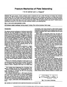
∆G1 (A1 → A2 ) and ∆G2 (A1 → A2 ) are calculated from the assumed stress state or strain state approximations, respectively. In some example calculations given in the next section, it was found that ∆G1 (A1 → A2 ) and ∆G2 (A1 → A2 ) bound the exact results. Thus they can be suggested as providing non-rigorous or practical bounds to ∆G(A1 → A2 ). One consequence of analyzing fracture events instead of continuous crack growth, is that the analysis must pay attention to loading conditions. Figure (1) shows a load-displacement curve for a fracture experiment with no residual stress effects. The hysteresis area between the loading and unloading curves is the total energy released during the fracture event. This area, however, depends on the loading conditions. The area of the ABC triangle is the total energy released by a fracture event at constant load. The shaded area of the ABD triangle is the total energy release by a fracture event at constant displacement. Thus the energy released at constant load is larger than the energy released at constant displacement. Deriving the slopes of the initial loading curve from Ei and of the unloading curve from Ef , it is easy to show the the ratio of the ABD to ABC triangular areas is Ef /Ei . In conventional fracture mechanics, or the limit as ∆A → 0, Ef will approach Ei or the energy released will be identical for constant load or constant displacement boundary conditions. In finite fracture mechanics, however, the loading conditions matter. Most laboratory experiments are done under displacement control; finite fracture mechanics analyses for such experiments should be done by analyzing constant displacement loading. AN EXAMPLE When cross-ply laminates ([0n /90m ]s or [90m /0n ]s ) are loaded in tension parallel to the 0◦ plies, the 90◦ plies develop transverse cracks or matrix microcracks (see review article Ref. (2)). On continued loading, the 90◦ plies crack into a roughly periodic array of microcracks. Early work on microcracking suggested microcracks form when the stress in the 90◦ plies reaches the transverse strength of the plies (14). Such a strength model does a poor job of explaining experimental results (15). It is now accepted that microcracking experiments can be better explained by a finite fracture mechanics model that assumes the next microcrack forms when the energy release rate for formation of that microcrack reaches Gmc or the critical microcracking toughness of the composite (2, 15). 4
Load
B
C
,,,,,,,,,,,,,,,,,,, ,,,,,,,,,,,,,,,,,,, ,,,,,,,,,,,,,,,,,,, ,,,,,,,,,,,,,,,,,,, ,,,,,,,,,,,,,,,,,,, ,,,,,,,,,,,,,,,,,,, ,,,,,,,,,,,,,,,,,,, ,,,,,,,,,,,,,,,,,,, ,,,,,,,,,,,,,,,,,,, ,,,,,,,,,,,,,,,,,,, ,,,,,,,,,,,,,,,,,,, ,,,,,,,,,,,,,,,,,,, ,,,,,,,,,,,,,,,,,,,D ,,,,,,,,,,,,,,,,,,, ,,,,,,,,,,,,,,,,,,, ,,,,,,,,,,,,,,,,,,, ,,,,,,,,,,,,,,,,,,, ,,,,,,,,,,,,,,,,,,, ,,,,,,,,,,,,,,,,,,, ,,,,,,,,,,,,,,,,,,, ,,,,,,,,,,,,,,,,,,, ,,,,,,,,,,,,,,,,,,, A ,,,,,,,,,,,,,,,,,,, ,,,,,,,,,,,,,,,,,,, ,,,,,,,,,,,,,,,,,,, ,,,,,,,,,,,,,,,,,,,
Displacement
Fig. 1. Load-displacement curve for a finite increase in crack area. The area of the ABC triangle is the total energy released by crack growth under load control. The shaded area of the ABD triangle is the total energy released by crack growth under displacement control.
Previous analyses of microcracking have derived approximate, 2D, plane-stress solutions to the stresses in the x−z plane of a microcracked laminate based either on an admissible stress state (16) or an admissible strain state (17). These analyses, as well as other shear-lag based analyses (18), have been implemented in finite fracture mechanics models, but these fracture models have all considered constant load conditions. Reference (1) has recently extended the admissible stress and admissible strain solutions to also consider constant displacement boundary conditions and used those results to derive a finite fracture mechanics analysis at constant displacement. Because most experiments are done at some fixed displacement rate, the constant displacement analysis is the more appropriate analysis for interpreting experiments. Below is a discussion of the new constant displacement analysis and some new analyses of experiments using either the the new constant displacement analysis or the previous constant load analysis. By making only one assumption, that the axial stresses in each are ply are only a function of the axial direction, and minimizing the complementary energy, it is possible to derive an approximate solution based on an admissible stress state (1, 16). From this analysis, the approximate change in complementary energy and constant displacement due to formation of n microcracks is (1) ³
0 ∆Γa (0 → n) = 2W t21 σxx,1
´2
Ã
C3
n L (ρ ) X EA i i=1
E0
!
χL (ρi )
(13)
0 where W is the width of the laminate, t1 is the semi-thickness of the 90◦ ply group, σxx,1 ◦ is the stress in the 90 plies prior to any damage, C3 is a constant that depends on ply meL (ρ ) is the lower-bound modulus of a cracked chanical properties and laminate geometry, EA i laminate with periodic microcrack intervals having aspect ratios ρi , E0 is the modulus of the undamaged laminate, and χL (ρi ) is a function of laminate properties and the current crack L (ρ ) are given elsewhere (2, 15). Similarly, by density. C3 , χL (ρi ), and a definition of EA i making a few assumptions about displacements, and minimizing the potential energy, it is possible to derive an approximate solution based on an admissible strain state (1, 17). From this analysis, the approximate change in potential energy due to formation of n microcracks
5
0.10 0.09
∆Gm (Upper Bound)
0.08
Gm (J/m2)
0.07 0.06
∆ Gm1
0.05 0.04 0.03 0.02
∆Gm2
0.01 0.00 -0.01 0.0
∆Gm (Lower Bound) 0.2
0.4 0.6 Crack Density (1/mm)
0.8
1.0
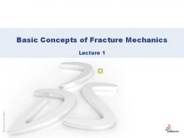
Fig. 2. Rigorous (upper and lower bounds) and practical bounds (∆Gm1 and ∆Gm2 ) for the energy release rate ∆Gm (n → n + 1) or the energy released due to the formation of the next microcrack. The symbols are finite element analysis calculations for ∆Gm (n → n + 1).
is (1) ∆Πa (0 → n) =
2W t21
³
0 σxx,1
´2
Ã
C3
n U (ρ ) X EA i i=1
E0
!
χU (ρi )
(14)
U (ρ ) is the upper-bound modulus to a cracked laminate with periodic microcrack where EA i intervals having aspect ratios ρi and and χU (ρi ) is a new function of laminate properties U (ρ ) are given elsewhere (1, 17). and the current crack density. χU (ρi ) and a definition of EA i
The total energy release rate due to formation of the (n + 1)th microcrack after previously forming n microcracks can simply be rigorously bounded from Eq. (10) by using A2 − A1 = 2W t1 . Similarly, substitution into Eqs. (11) and (12) leads to two practical bounds of ∆Gm1 (n → n + 1) = C3 t1
³ ³
0 σxx,1
0 ∆Gm2 (n → n + 1) = C3 t1 σxx,1
´2 ´2
Ã
!
E L (ρ/2) E L (ρ) 2 A χL (ρ/2) − A χL (ρ) E0 E0
Ã
(15) !
E U (ρ/2) E U (ρ) 2 A χU (ρ/2) − A χU (ρ) E0 E0
(16)
These practical bounds differ from previous practical bounds (see Refs. (15) and (17)) by L (ρ)/E and E U (ρ)/E ) which convert the previous constant the modulus ratio factors (EA 0 0 A load analyses to new constant displacement analyses. Figure 2 gives a sample calculation of ∆Gm (n → n + 1) for [0/902 ]s E-glass/epoxy laminate (properties in Ref. (17)) as a function 0 of crack density for loading conditions giving σxx,1 = 1 MPa. These sample calculations include the rigorous upper and lower bounds (from Eq. (10)) and the practical bounds defined in Eqs. (15) and (16). The symbols give some finite element calculations of the energy release rate. The rigorous upper and lower bounds bound the numerical FEA results but are fairly far apart. The practical bounds are much tighter and always bound the numerical results, but the sense of which practical bound is an upper bound and which is a lower bound switches at a crack density of about 0.6 mm−1 . To compare finite fracture mechanics predictions to experimental results, we first rewrite ∆Gm as ³ ´2 0 Gm,unit (D) (17) ∆Gm = σxx,1 6
where Gm,unit (D) is the energy release rate when there is unit initial axial stress in the 90◦ 0 plies and the current crack density is D. In linear thermoelasticity, σxx,1 can be written as (1)
(1)
0 = km σ0 + kth ∆T where σ0 is total applied stress, ∆T is the temperature differential σxx,1 (1)
(1)
leading to residual stresses, and km and kth are mechanical and thermal stiffness terms that can be derived from laminated plate theory (2). Equating ∆Gm to Gmc , using the 0 expanded form for σxx,1 , and rearranging gives (1)
−
km
σ (1) 0 kth
=−
s
1 (1) kth
Gmc + ∆T Gm,unit (D)
(18)
This equation suggests defining reduced stress and reduced crack density as (1)
σred = −
km
Dred = −
1
which leads to
σ (1) 0
kth
(19)
s
(1) kth
1
(20)
Gm,unit (D)
p
σred = Dred Gmc + ∆T
(21)
For a given laminate material, Eq. (21) defines a microcracking master plot (15). When a collection of experimental results from a variety of laminates of the same material are plotted √ as a master plot, Eq. (21) predicts the resulting plot should be linear with a slope of Gmc and an intercept giving the residual stress term ∆T (15). A master plot analysis of microcracking experiments critically tests the fundamental finite fracture mechanics hypothesis that the toughness property, Gmc , can be treated as a material property, or at least an effective material property, that is independent of the laminate structure and the current damage state. Moreover, a master plot analysis can be done with any input theory for Gm,unit (D) and thus can also test the validity of the energy release rate theory (15). The master plot method was previously used to analyze experimental results on a variety of [0n /90m ]s and [90m /0n ]s laminates made from AS4/3501-6 carbon/epoxy prepreg (15). That master plot analysis calculated Gm,unit (D) using a complementary energy analysis with constant load boundary conditions. Here those results will be compared to a new master plot analysis using constant displacement boundary conditions. The required constant displacement results for Gm,unit (D) for each laminate type are Ã
For [0n /90m ]s :
Gm,unit (D) = C3 t1
!
E L (ρ/2) E L (ρ) 2 A χL (ρ/2) − A χL (ρ) E0 E0 Ã
For [90m /0n ]s :
Gm,unit (D) =
(22) !
1 E L (ρ/3) E L (ρ) χa (ρ/3) − A χa (ρ) C3a t1 3 A 2 E0 E0
(23)
The alternate form for Gm,unit (D) for [90m /0n ]s is required to account for the different stress state in such laminates and the observation of staggered microcracks in the two surface 90◦ ply groups (19). The new constant, C3a and the new function χa (ρ) are defined in Ref. (19); furthermore, the Gm,unit (D) here is modified from the analysis in Ref. (19) by inclusion of the modulus ratio terms that are needed to convert the previous analysis to a constant displacement analysis. Finally, the following master plot analysis was done using Gm,unit (D) calculated from a complementary energy analysis, because it is currently the only analysis that can handle both [0n /90m ]s and [90m /0n ]s laminates and account for their different stress and damage states. 7
600
Reduced Stress (ßC)
500
Gmc = 220 J/m2 ∆T = -95˚C
400 300 200 100 0 0
5
10
15 20 25 30 Reduced Density (˚C m √J)
35
40
Fig. 3. Master plot analysis for 14 [0n /90m ]s (open symbols) and [90m /0n ]s (filled symbols) AS4/3501-6 carbon/epoxy laminates. Gm,unit (D) was calculated from a complementary energy analysis with constant displacement boundary conditions. The straight line is a linear fit to the experimental results. The slope and intercept of the fit give Gmc = 220 J/m2 and ∆T = −95◦ C.
Figure 3 gives the master plot for 14 different AS4/3501-6 laminates using Gm,unit (D) based on constant displacement boundary conditions. The open symbols are the results for [0n /90m ]s laminates; the filled symbols are the results for [90m /0n ]s laminates. Microcracking experiments sometimes show deviations from predictions at low crack density. These deviations have previously been attributed to either flaws or heterogeneity in toughness that cause the first few cracks to form sooner then expected (2, 15). To avoid this early data, the master plot was constructed using only experimental results having crack densities greater than 0.4 mm−1 . All experimental results conform very well to a linear master plot which suggests both that finite fracture mechanics can explain a wide variety of microcracking experiments and that Gm,unit (D) can be accurately calculated from a complementary energy analysis. Notably, the raw experimental results for [0n /90m ]s and [90m /0n ]s laminates with the same values of m and n are different, but converge to the same master plot. In other words, finite fracture mechanics analysis of microcracking can explain the difference in microcracking properties for laminates with central 90◦ plies vs. laminates with surface 90◦ plies. Figure 4 gives a master plot identical to Fig. 3 except Gm,unit (D) was calculated using constant load boundary conditions instead of constant displacement boundary conditions. The constant load results can be recovered from Eqs. (22) and (23) by dropping all modulus ratio terms. This master plot is identical to the one given in Ref. (15). It was previously judged to be a good analysis and gave superior results to all other theories for Gm,unit (D) tried at that time. By comparing, Figs. 3 and 4, however, it is clear that the constant displacement analysis improves the results even further and gives a master plot where experimental results conform even closer to a single line. The improvement on using a constant displacement analysis is satisfying because all experiments were done under displacement control. As described above, finite fracture mechanics calculations need to pay attention to boundary conditions. The best finite fracture mechanics analysis of microcracking is the one that uses the correct loading conditions. It would be interesting to do microcracking experiments under load control and see if finite fracture mechanics can explain any observed 8
600
Reduced Stress (ßC)
500
Gmc = 330 J/m2 ∆T = -143˚C
400 300 200 100 0 0
5
10
15 20 25 30 Reduced Density (˚C m √J)
35
40
Fig. 4. Master plot analysis for 14 [0n /90m ]s (open symbols) and [90m /0n ]s (filled symbols) AS4/3501-6 carbon/epoxy laminates. Gm,unit (D) was calculated from a complementary energy analysis with constant load boundary conditions. The straight line is a linear fit to the experimental results. The slope and intercept of the fit give Gmc = 330 J/m2 and ∆T = −143◦ C.
differences from the corresponding experiments under displacement control. CONCLUSION Finite fracture mechanics analysis of composite fracture events is, at least sometimes, a valid method for predicting composite failure. It clearly works for analysis of matrix microcracking. Some other applications of finite fracture mechanics that seem to be successful are analysis of instantaneous debonding following fiber breaks (1, 3) and cracking of paints or coatings on substrates (8–10). There are probably also examples of fracture events for which ∆K/∆A is irreproducible or variable from event to event and therefore finite fracture mechanics would not work. One simple example is tensile failure of unnotched specimens where the fracture event is complete fracture. Thus, in conclusion finite fracture mechanics is a potential tool for analysis of failure processes characterized by fracture events rather than by continuous crack growth. Before it can be used with confidence for any type of fracture event, however, it must be verified that a fracture event toughness deduced from experimental results can be treated as an effective material property. Acknowledgments This work was supported by a grant from the Mechanics of Materials program at the National Science Foundation (CMS-9713356). References 1. Nairn J. A., Int. J. Fract. (1999) submitted. 2. Nairn J. A., Hu S., in ‘Damage Mechanics of Composite Materials’, R. Talreja (ed.), Elsevier, Amsterdam (1994) 187. 3. Zhou X.-F., Nairn J. A., Wagner, H. D., Composites (1998) submitted. 4. Kanninen M. F., Popelar C.H., ‘Advanced Fracture Mechanics’, Oxford University Press (New York), 1985. 9
5. Hashin Z., J. Mech. Phys. Solids 44 (1996) 1129. 6. O’Brien T. K., in ‘Delamination and Debonding of Materials’, W. S. Johnson (ed.), ASTM STP 876 (1985) 282. 7. Nairn J. A., Liu Y. C., Composite Interfaces 4 (1997) 241. 8. Nairn J. A., Kim S. R., Engineering Fracture Mechanics 42 (1992) 195. 9. Kim S. R., Nairn J. A., Engineering Fracture Mechanics (1998) submitted. 10. Kim S. R., Nairn J. A., Engineering Fracture Mechanics (1998) submitted. 11. Griffith A. A., Philosophical Transactions Series A 221 (1920) 163. 12. Irwin G. R., Sagamore Research Conference Proceedings 2 (1956) 289. 13. Hashin Z., Shtrikman S., J. Mech. Phys. Solids 11 (1963) 127. 14. Garrett K. W., Bailey J. E., J. Mater. Sci 12 (1977) 157. 15. Nairn J. A., Hu S., Bark J. S., J. Mater. Sci. 28 (1993) 5099. 16. Hashin Z., Mech. of Mater. 4 (1985) 121. 17. Nairn J. A., Proc. of the 10th International Conference on Composite Materials I (1995) 423. 18. Parvizi A., Garrett K. W., Bailey J. E., J. Mater. Sci. 13 (1978) 195. 19. Nairn J. A., Hu S., Eng. Fract. Mech. 41 (1992) 203. (Note: preprints or the current status of “submitted” papers can be found on the internet at www.mse.utah.edu/~nairn/index.html)
10


![[PDF] Fracture Mechanics: Fundamentals and Applications, Third ...](https://m.moam.info/img/260x300/pdf-fracture-mechanics-fundamentals-and-applicatio_64784ad2097c474e708ca668.jpg)

![[PDF] Download Fracture Mechanics: Fundamentals and Applications ...](https://m.moam.info/img/260x300/pdf-download-fracture-mechanics-fundamentals-and-a_64771605097c474d228ba2a8.jpg)


![[PDF] Fracture Mechanics: Fundamentals and Applications, Third ...](https://m.moam.info/img/260x300/pdf-fracture-mechanics-fundamentals-and-applicatio_6478281d097c474b228ce13e.jpg)