Applications of Higher-Order Optimal Newton Secant Iterative Methods

Hindawi Publishing Corporation ISRN Applied Mathematics Volume 2013, Article ID 785287, 10 pages http://dx.doi.org/10.1155/2013/785287

Research Article Applications of Higher-Order Optimal Newton Secant Iterative Methods in Ocean Acidification and Investigation of Long-Run Implications of CO2 Emissions on Alkalinity of Seawater D. K. R. Babajee1 and V. C. Jaunky2 1 2

Scientific & Academic Research Council, African Network for Policy Research & Advocacy for Sustainability, Midlands, Mauritius Department of Business Administration, Technology and Social Sciences, Lule˚a University of Technology, SE-971 87 Lule˚a, Sweden

Correspondence should be addressed to V. C. Jaunky; [email protected] Received 3 April 2013; Accepted 4 May 2013 Academic Editors: C.-H. Lien and F. Tadeo Copyright © 2013 D. K. R. Babajee and V. C. Jaunky. This is an open access article distributed under the Creative Commons Attribution License, which permits unrestricted use, distribution, and reproduction in any medium, provided the original work is properly cited. The Newton secant method is a third-order iterative nonlinear solver. It requires two function and one first derivative evaluations. However, it is not optimal as it does not satisfy the Kung-Traub conjecture. In this work, we derive an optimal fourth-order Newton secant method with the same number of function evaluations using weight functions and we show that it is a member of the King family of fourth-order methods. We also obtain an eighth-order optimal Newton-secant method. We prove the local convergence of the methods. We apply the methods to solve a fourth-order polynomial arising in ocean acidifications and study their dynamics. We use the data of CO2 available from the National Oceanic and Atmospheric Administration from 1959 to 2012 and calculate the pH of the oceans for these years. Finally we further investigate the long-run implications of CO2 emissions on alkalinity of seawater using fully modified ordinary least squares (FMOLS) and dynamic OLS (DOLS). Our findings reveal that a one-percent increase in CO2 emissions will lead to a reduction in seawater alkalinity of 0.85 percent in the long run.

1. Introduction Recent advancements in the study of higher-order multipoint methods have made this field of research very active. Much literature on the multipoint Newton-like methods for function of one variable and their convergence analysis can be found in [1] and the historical developments of the methods in [2]. Newton secant method is a third-order two-point method and it was rediscovered in [3] as a leapfrog Newton method. However, it is not optimal because the order of an optimal method with 3 function evaluations should be 4 according to the Kung-Traub conjecture. In this work, we derive an optimal fourth-order Newton secant method with same number of function evaluations using weight functions and we show that it is a member of the King family of fourth-order methods. We also obtain an eighthorder optimal Newton secant method. We prove the local convergence of the methods. We apply the methods to solve a fourth-order polynomial arising in ocean acidifications and

study their dynamics. We use the data of CO2 available from the National Oceanic and Atmospheric Administration from 1959 to 2012 and calculate the pH of the oceans for these years. Finally, we further investigate the long-run implications of CO2 emissions on alkalinity of seawater using fully modified ordinary least squares (FMOLS) and dynamic OLS (DOLS).

2. Developments of the Methods Let 𝑥𝑛+1 = 𝜓(𝑥𝑛 ) define an iterative function (IF). Definition 1 (see [4]). If the sequence {𝑥𝑛 } tends to a limit 𝑥∗ in such a way that lim

𝑥𝑛+1 − 𝑥∗

𝑛 → ∞ (𝑥 𝑛

𝑝

− 𝑥∗ )

=𝐶

(1)

for 𝑝 ≥ 1, then the order of convergence of the sequence is said to be 𝑝, and 𝐶 is known as the asymptotic error constant.

2

ISRN Applied Mathematics

If 𝑝 = 1, 𝑝 = 2, or 𝑝 = 3, then the convergence is said to be linear, quadratic, or cubic, respectively. Let 𝑒𝑛 = 𝑥𝑛 − 𝑥∗ , and then the relation 𝑒𝑛+1 =

𝐶𝑒𝑛𝑝

+

𝑂 (𝑒𝑛𝑝+1 )

=

𝑂 (𝑒𝑛𝑝 ) .

(2)

is called the error equation. The value of 𝑝 is called the order of convergence of the method. Definition 2 (see [5]). The efficiency index is given by EI = 𝑝1/𝑑 ,

(3)

where 𝑑 is the total number of new function evaluations (the values of 𝑓 and its derivatives) per iteration. Let 𝑥𝑛+1 be determined by new information at 𝑥𝑛 , 𝜙1 (𝑥𝑛 ), . . . , 𝜙i (𝑥𝑛 ), 𝑖 ≥ 1. No old information is reused. Thus, 𝑥𝑛+1 = 𝜓 (𝑥𝑛 , 𝜙1 (𝑥𝑛 ) , . . . , 𝜙i (𝑥𝑛 )) .

(4)

Kung-Traub Conjecture (see [6]). Let 𝜓 be an IF without memory with 𝑑 evaluations. Then (5)

where 𝑝opt is the maximum order. The Newton (also called Newton-Raphson) IF (2nd NR) is given by 𝜓2nd NR (𝑥) = 𝑥 − 𝑢 (𝑥) ,

𝑓 (𝑥) . 𝑢 (𝑥) = 󸀠 𝑓 (𝑥)

(6)

The 2nd NR IF is one-point IF with 2 function evaluations and it satisfies the Kung-Traub conjecture 𝑑 = 2. The Halley IF (3rd Hal) is given by 𝑓󸀠󸀠 (𝑥) 𝑐2 (𝑥) = . 2𝑓󸀠 (𝑥) (7)

𝑢 (𝑥) 𝜓3rd Hal (𝑥) = 𝑥 − , 1 − 𝑐2 (𝑥) 𝑢 (𝑥)

It is one-point IF with 3 function evaluations and EI3rd Hal = 1.44 > EI2nd NR = 1.41. However, we need to calculate the second derivatives which can be computationally expensive for complex functions. A remedy to this is the Newton-secant IF (3rd NS) which can be written as 𝜓3rd NS (𝑥) = 𝑥 −

𝑓 (𝑥) 𝑢 (𝑥) . 𝑓 (𝑥) − 𝑓 [𝜓2nd NR (𝑥)]

1 , 1 − 𝑡1

𝑡1 =

1 + 𝑡1 2 . 1 − 𝑡1

(10)

Since EI4th NS = 41/3 = 1.59, the 4th NS has a higher efficiency index. It is remarkable by just multiplying the last term of (9) by the weight function, 1 + 𝑡1 2 , and we could increase the order from 3 to 4. This IF is similar to the member 𝛽 = 1 of the one-parameter King family of fourth-order IF [8] given by 𝜓4th FK (𝑥) = 𝜓2nd NR (𝑥) −

𝑓 (𝜓2nd NR (𝑥)) 1 + 𝛽𝑡1 . 𝑓󸀠 (𝑥) 1 + (𝛽 − 2) 𝑡1 (11)

Based on King-type family higher-order IFs [9], an eighthorder 8th NS IF can be given by 𝜓8th NS (𝑥) = 𝑥 −

𝑓󸀠

1 + 𝑡1 + 1.5𝑡1 2 1 ( + 4𝑡2 + 𝑡3 ) , (𝑥) 1 − 𝑡1 + 0.5𝑡1 2

where 𝑡2 =

𝑓 (𝜓4th NS (𝑥)) , 𝑓 (𝑥)

𝑓 [𝜓2nd NR (𝑥)] . 𝑓 (𝑥) (9)

𝑡3 =

𝑓 (𝜓4th NS (𝑥)) . 𝑓 (𝜓2nd NR (𝑥))

(13)

The 8th NS IF is an optimal IF which satisfies the Kung-Traub conjecture with EI8th NS = 51/4 = 1.68 which is the highest efficiency index among all IFs considered in this work.

3. Convergence Analysis Theorem 3. Let a sufficiently smooth function 𝑓 : 𝐷 ⊂ R → R have a simple root 𝑥∗ in the open interval 𝐷. Then the 4th NS IF (10) is of local fourth-order convergence and the 8th NS IF (12) is of local eighth-order convergence. Proof. Let 𝑐𝑗 = 𝑓(𝑗) (𝑥∗ )/𝑗!𝑓󸀠 (𝑥∗ ), 𝑗 = 2, 3, 4. Using the Taylor series and the symbolic software such as, Maple we have 𝑓 (𝑥) = 𝑓󸀠 (𝑥∗ ) [𝑒𝑛 + 𝑐2 𝑒𝑛2 + 𝑐3 𝑒𝑛3 + 𝑐4 𝑒𝑛4 + ⋅ ⋅ ⋅ ] ,

(14)

𝑓󸀠 (𝑥) = 𝑓󸀠 (𝑥∗ ) [1 + 2𝑐2 𝑒𝑛 + 3𝑐3 𝑒𝑛2 + 4𝑐4 𝑒𝑛3 + ⋅ ⋅ ⋅ ] ,

(15)

so that 𝑢 (𝑥) = 𝑒𝑛 − 𝑐2 𝑒𝑛2 + 2 (𝑐22 − 𝑐3 ) 𝑒𝑛3 + (7𝑐2 𝑐3 − 4𝑐23 − 3𝑐4 ) 𝑒𝑛4 + ⋅ ⋅ ⋅ ,

(8)

It has the same efficiency as the 3rd Hal IF but it requires 2𝑓 and 1𝑓󸀠 evaluations, hence no second derivatives, and is a also variant of 3rd Hal IF [7]. However, it does not satisfy the Kung-Traub conjecture. In this work, we develop a fourthorder Newton-secant IF with 3 functions evaluations using weight functions. The 3rd NS’s IF can be written as 𝜓3rd NS (𝑥) = 𝑥 − 𝑢 (𝑥)

𝜓4th NS (𝑥) = 𝑥 − 𝑢 (𝑥)

(12)

Then 𝜓 is called a multipoint IF without memory.

𝑝 (𝜓) ≤ 𝑝opt = 2𝑑−1 ,

The 4th NS IF can be given by

𝜓2nd NR (𝑥) − 𝑥∗ = 𝑐2 𝑒𝑛2 − 2 (𝑐22 − 𝑐3 ) 𝑒𝑛3 − (7𝑐2 𝑐3 − 4𝑐23 − 3𝑐4 ) 𝑒𝑛4 + ⋅ ⋅ ⋅ .

(16)

(17)

Now, the Taylor expansion of 𝑓(𝑦) about 𝑥∗ gives 𝑓 (𝑦) = 𝑓󸀠 (𝑥∗ ) × [(𝑦 − 𝑥∗ ) + 𝑐2 (𝑦 − 𝑥∗ ) 3

2

(18) 4

+ 𝑐3 (𝑦 − 𝑥∗ ) + 𝑐4 (𝑦 − 𝑥∗ ) + ⋅ ⋅ ⋅ ] .

ISRN Applied Mathematics

3

Using (14), (18), and (17), we have 𝑡1 =

a series of chemical changes that ultimately leads to increased hydrogen ion concentration, denoted subsequently as [H+ ], and thus acidification (see [12, 13]). This increase in [H+ ] is manifest as a decrease in pH; note that [H+ ] and pH move in opposite directions due to the following basic relation:

𝑓 [𝜓2nd NR (𝑥)] 𝑓 (𝑥)

= 𝑐2 𝑒𝑛 + (2𝑐3 − 3𝑐2 2 ) 𝑒𝑛2 + (3𝑐4 − 10𝑐2 𝑐3 +

pH = −log10 [H+ ] .

8𝑐2 ) 𝑒𝑛3 3

(23)

𝜓8th NS (𝑥) − 𝑥∗

Ocean acidification is the name given to the ongoing decrease in the pH of the Earth’s oceans, caused by their uptake of anthropogenic carbon dioxide from the atmosphere [14]. Between 1751 and 1994, surface ocean pH is estimated to have decreased from approximately 8.179 to 8.104 (a change of −0.075) [15]. A decrease in ocean pH of 0.1 units corresponds to a 30% increase in the concentration of H+ in seawater, assuming that alkalinity and temperature remain constant [16, p. 406]. There is about fifty times as much carbon dissolved in the oceans in the form of CO2 and carbonic acid, bicarbonate, and carbonate ions as that in the atmosphere. The oceans act as an enormous carbon sink and have taken up about a third of CO2 emitted by human activity [17]. Most of the CO2 taken up by the ocean forms carbonic acid in equilibrium with bicarbonate and carbonate ions. Some is consumed in photosynthesis by organisms in the water, and a small proportion of that sinks and leaves the carbon cycle. Increased CO2 in the atmosphere has led to decreasing alkalinity of seawater and there is concern that this may adversely affect organisms living in the water. In particular, with decreasing alkalinity, the availability of carbonates for forming shells decreases [18, p. 125], although there is evidence of increased shell production by certain species under increased CO2 content [19].

1 = ( 𝑐2 (−𝑐3 + 3𝑐2 2 ) (65𝑐2 4 − 34𝑐3 𝑐2 2 + 2𝑐2 𝑐4 + 2𝑐3 2 )) 𝑒𝑛8 2

4.2. Ocean Chemistry [2]. We begin with CO2 dissolving in H2 O to form carbonic acid, H2 CO3 as

+ (−14𝑐2 𝑐4 + 37𝑐3 𝑐2 2 − 20𝑐2 4 − 8𝑐3 2 + 4𝑐5 ) 𝑒𝑛4 + ⋅ ⋅ ⋅ , (19) so that by using computer algebra software such as Maple we get 𝜓3th NS (𝑥) − 𝑥∗ = 𝑐2 2 𝑒𝑛3 + ⋅ ⋅ ⋅ , 𝜓4th NS (𝑥) − 𝑥∗ = 𝑐2 (−𝑐3 + 3𝑐2 2 ) 𝑒𝑛4 + ⋅ ⋅ ⋅ .

(20)

Similarly, we have 𝑡2 = 𝑐2 (−𝑐3 + 3𝑐2 2 ) 𝑒𝑛3 + (−2𝑐2 𝑐4 − 2𝑐3 2 + 21𝑐3 𝑐2 2 − 21𝑐2 4 ) 𝑒𝑛4 + ⋅ ⋅ ⋅ , 𝑡3 = (−𝑐3 + 3𝑐2 2 ) 𝑒𝑛2

(21)

+ (−2𝑐4 + 12𝑐2 𝑐3 − 12𝑐2 3 ) 𝑒𝑛3 + ⋅ ⋅ ⋅ , so that finally we get

+ ⋅⋅⋅ .

CO2 + H2 O 󴀕󴀬 H2 CO3 . (22)

4. Ocean Acidification 4.1. Introduction [2]. The accumulation of greenhouse gases (GHGs) in the Earth’s atmosphere is now a major topic of discussion to anticipate changes in the Earth’s climate. The GHGs cause a reduction in the reradiation of energy from the Sun back into the outer space. Since less energy leaves the Earth’s atmosphere, heating of the atmosphere results as a manifest in a temperature rise [12]. This temperature rise, the so-called global warming, is in turn a driving force for climate change. CO2 is the major GHG, with increasing levels primarily from the burning of fossil fuels. Thus, changes in the CO2 level or concentration in the Earth’s atmosphere are of paramount importance in understanding anticipated warming and climate change. A second aspect of CO2 accumulation in the atmosphere that is not as generally recognized and appreciated as temperature rise is the accumulation of carbon (from CO2 ) in the oceans that leads to ocean acidification. CO2 dissolves in ocean water and undergoes

(24)

The double arrow 󴀕󴀬 denotes a reversible chemical reaction (a reaction that can proceed either forward to produce H2 CO3 or backward to produce CO2 and H2 O). A common convention is to take [CO2 ] as the dissolved CO2 , denoted as [CO2 ]aq , plus the carbonic acid [H2 CO3 ]aq . Carbonic acid is a weak acid which in turn dissociate into bicarbonate ions, HCO−3 , as H2 CO3 󴀕󴀬 H+ + HCO−3 .

(25)

Bicarbonate ions in turn dissociates into carbonate ions, CO2− 3 HCO−3 󴀕󴀬 H+ + CO2− 3 .

(26)

The reactions (25) and (26) produce hydrogen ions and therefore contribute to acidification. H2 O also dissociates to produce hydrogen ions as H2 O 󴀕󴀬 H+ + OH− .

(27)

Additionally, boron hydroxide in seawater dissociates to produce hydrogen ions as B(OH)3 + H2 O 󴀕󴀬 H+ + B(OH)−4 .

(28)

4

ISRN Applied Mathematics

In this work, we do not consider other compounds in the oceans that also dissociate to produce hydrogen ions. We explain how to compute [H+ ] and pH from the reactions (24) to (28). For the following analysis, we use the equilibrium constants of Bacastow and Keeling [20] expressed in the units of moles/litre. The relation between gaseous and liquid CO2 is 𝐾0 =

[CO2 ] = 3.347 (−5) , 𝑃𝑡

(39)

𝐾0 𝐾1 𝑃𝑡 2𝐾0 𝐾1 𝐾2 𝑃𝑡 𝐾W 𝐵𝐾B + + − [H+ ] + + + 2 + [H ] 𝐾B + [H ] [H+ ] [H ] (40)

which simplifies to the solution of a fourth-order polynomial given by 4

𝑛

𝑝 ([H+ ]) = ∑ 𝐷𝑛 [H+ ] ,

(41)

𝑛=0

where (30)

𝐷0 = 2𝐾0 𝐾1 𝐾2 𝑃𝑡 𝐾B , 𝐷1 = 𝐾0 𝐾1 𝑃𝑡 𝐾B + 2𝐾0 𝐾1 𝐾2 𝑃𝑡 + 𝐾W 𝐾B ,

[H+ ] [CO2− 3 ] [HCO−3 ]

= 8.501 (−10) .

𝐷2 = 𝐾0 𝐾1 𝑃𝑡 + 𝐵𝐾B + 𝐾W − 𝐴𝐾B , (31)

𝐾W = [H+ ] [OH− ] = 6.46 (−15) .

(32)

For reaction (28), [H+ ] [B(OH)−4 ] = 1.881 (−9) . [B(OH)3 ]

(33)

The alkalinity, 𝐴, which expresses the electrical neutrality of ocean water is defined as − − + 𝐴 = [HCO−3 ] + 2 [CO2− 3 ] + [B(OH)4 ] + [OH ] − [H ] . (34)

We can assume that the values of 𝐴 do not change with time [20]. From (29), we have [CO2 ] = 𝐾0 𝑃𝑡 .

(35)

𝐷3 = −𝐾B − 𝐴,

𝑧=

1 , [H+ ]

𝑧 ∈ Z,

(43)

and then the pH = log10 𝑧. We require to find the positive real solution of another fourth-order polynomial: (44)

𝑛=0

(36)

𝐾2 [HCO−3 ] 𝐾0 𝐾1 𝐾2 𝑃𝑡 = 2 [H+ ] [H+ ]

(37)

Similarly, we obtain

from (31) and (36). Using 𝐵 = [B(OH)3 ] + [B (OH)−4 ]

4.3. Dynamic Behaviour. We next study the dynamic behaviour of the methods in the complex plane Z to find the best starting points. For a given value of 𝑃𝑡 , polynomial 𝑝([H+ ]) in (41) has one positive real root (the one we are seeking), one negative real root, and two complex roots. Since these solutions have very small values except the negative one, it is difficult to study their polynomiography [23]. Instead, we consider the change of variable

4

𝐾1 [CO2 ] 𝐾0 𝐾1 𝑃𝑡 = . [H+ ] [H+ ]

[HCO−3 ] =

We use 𝐴 = 2.050 [22, p. 334] and 𝐵 = 0.409 [20, p. 131].

𝑝 (𝑧) = ∑ 𝐷4−𝑛 𝑧𝑛 .

From (30) and (35), we have

[CO2− 3 ]=

(42)

𝐷4 = −1.

For reaction (27),

𝐾B =

𝐵𝐾B . 𝐾B + [H+ ]

Substituting (32) and (35)–(39) into (34), we have

(29)

For reaction (26), 𝐾2 =

[B(OH)−4 ] =

𝐴=

where [CO2 ] is the sum of the dissolved CO2 and carbonic acid and 𝑃𝑡 is the gas phase CO2 partial pressure in ppm measured by the National Oceanic and Atmospheric Administration (NOAA) at the Mauna Loa Observatory, Hawaii [21], and 𝑎(−𝑏) denotes 𝑎 × 10−𝑏 . For reaction (25), [H+ ] [HCO−3 ] 𝐾1 = = 9.747 (−7) . [CO2 ]

in (33), we have

(38)

We draw the polynomiographs of 𝑝([H+ ]). Let 𝑧0 = 𝑥 + 𝑖𝑦, and let 𝑥, 𝑦 ∈ R be the initial point. A square grid of 65536 points, composed of 256 columns and 256 rows corresponding to the pixels of a computer display, would represent a region of the complex plane [24]. We consider the square R × R = [−1(9), 1(9)] × [−1(9), 1(9)]. Each grid point is used as a starting value 𝑧0 of the sequence 𝑧𝑘+1 = 𝜓IF (𝑧𝑘 ) and the number of iterations until convergence is counted for each grid point. We assign different colours to each root 𝑧𝑗∗ , 𝑗 = 1, 2, 3, 4 of 𝑝([H+ ]) if |𝑧𝑗∗ − 𝑧𝑘 | < 1(−4), in at most 25 iterations In this way, the basin of attraction for each

ISRN Applied Mathematics

−1

5

×109

−1

−0.8

−0.8

−0.6

−0.6

−0.4

−0.4

−0.2

×109

−0.2 ∗

0

∗ ∗

∗

0.2

0.2

0.4

0.4

0.6

0.6

0.8

0.8

1 −1

−0.5

0

∗

0

0.5

1 ×10

∗ ∗

∗

1 −1

−0.5

0

0.5

9

1 ×109

(a) 2nd NR

(b) 3rd NS

Figure 1: Polynomiographs of the 2nd NR and 3rd NS methods for the polynomial 𝑝(𝑧) with 𝑃𝑡 = 393.81.

1

×109

1

0.8

0.8

0.6

0.6

0.4

0.4

0.2 0 −0.2

0.2

∗

∗ ∗

∗

0 −0.2

−0.4

−0.4

−0.6

−0.6

−0.8

−0.8

−1 −1

×109

−0.5

0

0.5

1

×109

(a) 4th NS

−1 −1

∗

∗ ∗

∗

−0.5

0

0.5

1 ×109

(b) 8th NS

Figure 2: Polynomiographs of the 4th NS and 8th NS methods for the polynomial 𝑝(𝑧) with 𝑃𝑡 = 393.81.

root would be assigned a characteristic colour. The common boundaries of these basins of attraction constitute the Julia set of the IF If the iterates do not satisfy the above criterion for convergence, we assign the dark blue colour. Figures 1 and 2 show the polynomiographs of the 2nd NR, 3rd NS, 4th NS and 8th NS methods, respectively. In this case, the positive root of the polynomial, 𝑧∗ = 1.262801212073384(8) (coloured brownish yellow), corresponds to the solution [H+ ]∗ = 7.918902757133942(−9). It can be shown that there are diverging points for the

higher-order Newton-secant methods and that the 2nd NR method has the largest basins of attraction for the positive root among the 4 methods. But we are using the dynamics of the methods to find a suitable starting point for the higherorder Newton-secant methods so that we can make use of their higher-order convergence. Figures 3 and 4 show the basins of attractions on the real line of the 2nd NR, 3rd NS, 4th NS, and 8th NS methods, respectively, for the positive root of 𝑝(𝑧). They reveal that the 2nd NR will converge for a starting point 𝑧0 > 0.7(8). As the order of the method

6

ISRN Applied Mathematics

−1

×10−3

−1

−0.8

−0.8

−0.6

−0.6

−0.4

−0.4

−0.2

−0.2 ∗

0

0.2

0.4

0.4

0.6

0.6

0.8

0.8 1

∗

0

0.2

1 0.5

×10−3

1.5

2 ×10

1 0.5

1

1.5

8

2 ×108

(a) 2nd NR

(b) 3rd NS

Figure 3: Basins of attractions on the real line of the 2nd NR and 3rd NS methods for the positive root of 𝑝(𝑧).

1

×10−3

1

0.8

0.8

0.6

0.6

0.4

0.4

0.2

0.2 ∗

0

−0.2

−0.4

−0.4

−0.6

−0.6

−0.8

−0.8 1

∗

0

−0.2

−1 0.5

×10−3

1.5

2 ×10

(a) 4th NS

−1 0.5

1

1.5

8

2 ×10

8

(b) 8th NS

Figure 4: Basins of attractions on the real line of the 4th NS and 8th NS methods for the positive root of 𝑝(𝑧).

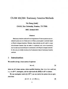
increase, the basins of attraction decrease and higher-order Newton-secant methods have difficulty to converge for some starting points. We also find that all methods will converge for the starting point 𝑧0 = 1.25(8) or [H+ ]0 = 8(−9). 4.4. Numerical Experiments and Results. We use the data available from NOOA to calculate the pH of the ocean from 1959 to 2012. We use a common starting point [H]+0 = 8(−9) for each 𝑃𝑡 and stop the methods whenever |[H]+𝑘+1 − [H]+𝑘 | < 1(−12) in at most 25 iterations. The approximate solutions

are calculated correctly to 16 digits in MATLAB. We denote by 𝑁𝑠 the number of successful points and by 𝜇 as the mean iteration number for the converging points. Table 2 gives a comparison in which we observe that the 3 methods successfully converge to the required root but the 8th NS method has a few diverging points. The 4th NS method is the most effective with the lowest mean iteration number and all converging points. Table 1 shows the calculated pH from 1959 to 2012. Figure 5 shows the variation of CO2 and pH with time. We observe that as the CO2 increases, the pH decreases.

7 400

8.19

390

8.18

380

8.17

370

8.16

360

8.15 pH

CO2 (ppm)

ISRN Applied Mathematics

350

8.14

340

8.13

330

8.12

320

8.11

310 1960

1980 2000 t (years)

8.1 1960

1980 2000 t (years)

Figure 5: Variation of CO2 and pH with time.

Table 1: pH of oceans using the 𝑃𝑡 from NOAA from 1959 to 2012. Time 1959 1960 1961 1962 1963 1964 1965 1966 1967 1968 1969 1970 1971 1972 1973 1974 1975 1976 1977 1978 1979 1980 1981 1982 1983 1984 1985

𝑃𝑡 315.98 316.91 317.64 318.45 318.99 319.62 320.04 321.38 322.16 323.04 324.62 325.68 326.32 327.45 329.68 330.17 331.08 332.05 333.78 335.41 336.78 338.68 341.11 341.22 342.84 344.41 345.87

pH 8.1794 8.1784 8.1776 8.1767 8.1761 8.1754 8.1749 8.1735 8.1726 8.1717 8.1699 8.1688 8.1681 8.1669 8.1645 8.1640 8.1630 8.1620 8.1602 8.1584 8.1570 8.1550 8.1525 8.1524 8.1507 8.1491 8.1476

Time 1986 1987 1988 1989 1990 1991 1992 1993 1994 1995 1996 1997 1998 1999 2000 2001 2002 2003 2004 2005 2006 2007 2008 2009 2010 2011 2012

𝑃𝑡 347.19 348.98 351.45 352.90 354.16 355.48 356.27 356.95 358.64 360.62 362.36 363.47 366.50 368.14 369.40 371.07 373.17 375.78 377.52 379.76 381.85 383.71 385.57 387.35 389.85 391.62 393.81

pH 8.1463 8.1444 8.1419 8.1405 8.1392 8.1379 8.1371 8.1364 8.1347 8.1328 8.1311 8.1300 8.1270 8.1254 8.1242 8.1226 8.1206 8.1181 8.1165 8.1144 8.1124 8.1107 8.1089 8.1073 8.1050 8.1033 8.1013

Table 2: Comparison of successful starting point and mean iteration number for each method. 𝑁𝑠 54 54 54 47

Method 2nd NR 3th NS 4th NS 8th NS

𝜇 3.7037 2.8704 2.7778 2.1852

Table 3: Unit root tests. ADF Series

DF-GLS

With With With With constant constant and constant and constant and and without trend with trend without trend with trend

log10 pH 3.412[0] log10 CO2 3.266[0] Δlog10 pH −2.291[3] Δlog10 CO2 −2.347[3]

−1.800[0] −1.894[0] −6.104[1]∗ −6.101[1]∗

−0.121[4] −0.147[1] −0.130[4] −0.188[1] −2.352[2]∗∗ −4.486[1]∗ −2.423[2]∗∗ −6.241[1]∗

Note: to select the order of lag, we start with a maximum lag length of 4 and pare it down as per the Akaike information criterion (AIC). There is no general rule on how to choose the maximum lag to start with. The bandwidth and maximum lag length are chosen according to the Bartlett kernel which is equal to 4(𝑇/100)2/9 ≈ 4, where 𝑇 = 54. The optimal lag length is given in square brackets. The MacKinnon critical values [10] for the ADF unit root tests with a constant and without a time are −3.59, −2.94, and −2.60 at 1%, 5%, and 10% significance level,respectively, while those with a constant and a time trend are −4.17, −3.51, and −3.19, respectively. DF-GLS critical values without trend at 1%, 5%, and 10% levels are −2.62, −2.26, and −1.95 and with a trend are −3.76, −3.17, and −2.87, respectively. The optimal lag is chosen according to the Akaike information criterion (AIC) and Schwarz Bayesian criterion for the ADF and DF-GLS tests, respectively. ∗ and ∗∗ denote 1% and 5% significance level correspondingly.

8

ISRN Applied Mathematics Table 4: Johansen cointegration test.

LR test 𝜆-max Tr

Null 𝑟=0 𝑟≤1 𝑟=0 𝑟≤1

Hypothesis Alternative 𝑟=1 𝑟=2 𝑟≥1 𝑟=2

Statistics

95% critical values

90% critical values

23.752∗∗ 4.773 28.525∗∗ 4.773

18.330 11.540 23.830 11.540

16.280 9.750 21.230 9.750

Note: the test is conducted with unrestricted constants and trends in the VAR model. 𝑟 is the number of cointegrating vectors. The optimal lag length is set to 4 according to the AIC.

4.5. Empirical Analysis of Impact of 𝐶𝑂2 on Alkalinity of Seawater. To empirically test the impact of CO2 in the atmosphere on the alkalinity of seawater, we set up the following generalized equation: pH = 𝑓 (CO2 , 𝜖) ,

Table 5: Long-run estimators. Series

(45)

where 𝜖 is the error term. The concept of cointegration as per Engle and Granger [25] is used to investigate any long-run relationship between nonstationary variables. Time-series data such as pH and CO2 tend to be nonstationary in levels. If a series is stationary, then the probability laws controlling its process are stable over time, that is, in statistical equilibrium [26]. In contrast, series having a unit root are nonstationary. Shocks have a unit root and can, in part, change the long-run level of the time series permanently. Per se, a series is said to be integrated of order 𝜐 or 𝐼(𝜐) if it were to be different by 𝜐 times to become stationary. A stationary process is a series which follows an 𝐼(0) process. To run the model, the logarithm of base 10 of the variables is taken. As a prerequisite of the cointegration test, the unit root properties of the two series are investigated. The augmented Dickey-Fuller (ADF) test as proposed by Dickey and Fuller [27] and the DFGLS test as per Elliott et al. [28] for the null of a unit root are considered. The DF-GLS test is a modified ADF test and tends to be a more asymptotically powerful test. These tests apply regressions which include a constant term only, while the other contain both a constant term and a time trend. Time series data tend to exhibit a trend over time and hence it is more appropriate to consider a regression with both a constant term and a trend. In contrast, first differencing is likely to remove any deterministic trends. Hence, the regression should include a constant only. In general, time-series data tends to be nonstationary and 𝐼(1). Both series must be integrated of the same order to validate a cointegrating relationship. The Johansen cointegration test [29] is conducted within a vector autoregression (VAR) structure and it involves two log-likelihood ratio (LR) test statistics, namely, the maximum eigenvalue (𝜆-max) and trace (Tr) statistics. Once a cointegrating relationship is established, long-run estimates can be computed via the fully modified ordinary least squares (FMOLS) and dynamic OLS (DOLS) of Phillips and Hansen [30] and Stock and Watson [31], respectively. Table 3 shows the results of the unit root tests. Both series are found to be nonstationary. The ADF test statistics illustrate an 𝐼(1) process for both series only when a trend is considered in the testing framework. However, when testing for a unit root using first-differenced

log10 CO2

Dependent log10 pH FMOLS DOLS Standard Standard Coefficient Coefficient deviation deviation −0.845∗

0.003

−0.849∗

0.009

Note: a constant and time trend are included in each model. The critical values of the two-tailed 𝑡-statistics test at 1%, 5%, and 10% significance levels are 2.326, 1.645, and 1.282, respectively. The maximum lag/lead is set to 2 [11].

data, the trend should be excluded. The DF-GLS confirms our a priori expectation. Both series are found to be 𝐼(1) for both deterministics. Table 4 reports the cointegration test statistics. According to the null hypothesis for the 𝜆-max and Tr tests, there are at most 𝑟 cointegrating vectors, whereas the alternative hypotheses are 𝑟 + 1 and at least 𝑟 + 1 for the 𝜆-max and Tr statistics, respectively. As per the 𝜆-max statistics, the null hypothesis of 𝑟 = 0 is rejected in favour of 𝑟 = 1. A similar result is found when referring to the Tr statistics as the null hypothesis of 𝑟 = 0 is rejected in favour of 𝑟 ≥ 1. The computed test statistics are 23.75 and 28.53 for the 𝜆-max and Tr tests, respectively. The null hypothesis of no cointegration is rejected at 5% level. Furthermore, the null hypothesis of at most one cointegrating vector (𝑟 ≤ 1) is in no case rejected in both cases. In sum, these findings provide evidence of a long-run equilibrium relationship between pH and CO2 . Given the presence of a cointegrating vector, the long-run elasticity can now be computed and is reported in Table 5. The FMOLS and DOLS methods are robust single equation approaches which can correct for endogeneity bias and serial correlation (The computed test statistic for serial correlation according to Durbin and Watson [32] is 𝑑-statistic (2, 54) = 0.021. This reveals positive serial correlation) in a semiparametric and parametric way, respectively. CO2 in the atmosphere has a statistically significant negative impact on the alkalinity of seawater and the long-run elasticities from both methods tend to coincide. For instance, a one-percent increase in CO2 emissions will generate to a reduction in seawater alkalinity of 0.85 percent in the long run.

5. Conclusion We develop an optimal fourth- and eighth-order Newtonsecant methods. We study their dynamics in a fourth-order polynomial arising in ocean acidification. We also perform an

ISRN Applied Mathematics investigation on the long-run implications of CO2 emissions on alkalinity of seawater using fully modified ordinary least squares (FMOLS) and dynamic OLS (DOLS). We find that a one-percent increase in CO2 emissions will lead to a reduction in seawater alkalinity of 0.85 percent in the long run. Put differently, a fall in CO2 emissions will lead to an improvement of the quality of seawater and therefore to the sustainability of the marine ecosystem.

Acknowledgments The authors are thankful to Pieter Tans for giving the permission to use the data published by the National Oceanic and Atmospheric Administration (NOAA). The authors are thankful to Robert Lundmark and Patrik S¨oderholm for their valuable suggestions and comments on the paper. The authors are also thankful to the unknown referees for their valuable comments to improve the paper.

References [1] J. F. Traub, Iterative Methods for the Solution of Equations, Prentice Hall, New Jersey, NJ, USA, 1964. [2] D. K. R. Babajee, Analysis of higher order variants of Newton’s method and their applications to differential and integral equations and in ocean acidification [Ph.D. thesis], University of Mauritius, 2010. [3] A. B. Kasturiarachi, “Leap-frogging Newton’s method,” International Journal of Mathematical Education in Science and Technology, vol. 33, no. 4, pp. 521–527, 2002. [4] R. Wait, The Numerical Solution of Algebraic Equations, John Wiley & Sons, 1979. [5] A. M. Ostrowski, Solutions of Equations and System of Equations, Academic Press, New York, NY, USA, 1960. [6] H. T. Kung and J. F. Traub, “Optimal order of one-point and multipoint iteration,” Journal of the Association for Computing Machinery, vol. 21, no. 4, pp. 643–651, 1974.

9 [13] G. W. Griffiths, A. J. McHugh, and W. E. Schiesser, “An introductory global CO2 model,” Chemical and Biochemical Engineering Quarterly, vol. 22, no. 2, p. 265, 2008. [14] K. Caldeira and M. E. Wickett, “Oceanography: anthropogenic carbon and ocean pH,” Nature, vol. 425, p. 365, 2003. [15] J. C. Orr, V. J. Fabry, O. Aumont et al., “Anthropogenic ocean acidification over the twenty-first century and its impact on calcifying organisms,” Nature, vol. 437, no. 7059, pp. 681–686, 2005. [16] N. L. Bindo, J. Willebrand, V. Artale et al., “Observations: oceanic climate change and sea level,” in Climate Change 2007: The Physical Science Basis. Contribution of Working Group I to the Fourth Assessment Report of the Intergovernmental Panel on Climate Change, S. Solomon, D. Qin, M. Manning et al., Eds., pp. 385–432, Cambridge University Press, New York, NY, USA, 2007. [17] S. C. Doney and N. M. Levine, How Long Can the Ocean Slow Global Warming? Oceanus, 2006, https://www.whoi.edu/ oceanus/viewArticle.do?id=17726. [18] T. S. Garrison, Oceanography: An Invitation to Marine Science, Thomson Brooks, 2004. [19] J. B. Ries, A. L. Cohen, and D. C. McCorkle, “Marine calcifiers exhibit mixed responses to CO2 -induced ocean acidification,” Geology, vol. 37, no. 12, pp. 1131–1134, 2009. [20] R. Bacastow and C. D. Keeling, “Atmospheric carbon dioxide and radiocarbon in the natural carbon cycle: changes from a.d. 1700 to 2070 as deduced from a geochemical model,” in Proeedings of the 24th Brookhaven Symposium in Biology, G. W. Woodwell and E. V. Pecan, Eds., pp. 86–133, The Technical Information Center, Office of Information Services, United State Atomic Energy Commission, Upton, NY, USA, May 1972. [21] P. Tans, Trends in carbon dioxide. National Oceanic and Atmospheric Administration Earth System Research Laboratory, 2009, http://www.esrl.noaa.gov/gmd/ccgg/trends/. [22] J. L. Sarmiento and N. Gruber, Ocean Biogeochemical Dynamics, Princeton University Press, Princeton, NJ, USA, 2006. [23] B. Kalantari, Polynomial Root-Finding and Polynomiography, World Scientific Publishing, Singapore, 2009.

[7] D. K. R. Babajee and M. Z. Dauhoo, “An analysis of the properties of the variants of Newton’s method with third order convergence,” Applied Mathematics and Computation, vol. 183, no. 1, pp. 659–684, 2006.

[24] E. R. Vrscay, “Julia sets and mandelbrot-like sets associated with higher order Schr¨oder rational iteration functions: a computer assisted study,” Mathematics of Computation, vol. 46, no. 173, pp. 151–169, 1986.

[8] R. F. King, “A family of fourth order methods for nonlinear equations,” SIAM Journal on Numerical Analysis, vol. 10, no. 5, pp. 876–879, 1973.

[25] R. F. Engle and C. W. J. Granger, “Cointegration and errorcorrection: representation, estimation and testing,” Econometrica, vol. 55, no. 2, pp. 251–276, 1978.

[9] D. K. R. Babajee and R. Thukral, “On a 4-point sixteenth-order king family of iterative methods for solving nonlinear equations,” International Journal of Mathematics and Mathematical Sciences, vol. 2012, Article ID 979245, 13 pages, 2012.

[26] W. Vandaele, Applied Time Series and Box-Jenkins Models, Academic Press, New York, NY, USA, 1983.

[10] J. G. McKinnon, “Critical values for cointegration tests,” in Long Run Relationships: Reading in Cointegration, pp. 1–16, Oxford University Press, 1991. [11] N. C. Mark and D. Sul, “Cointegration vector estimation by panel DOLS and long-run money demand,” Oxford Bulletin of Economics and Statistics, vol. 65, no. 5, pp. 655–680, 2003. [12] P. J. Bresnahan, G. W. Griffiths, A. J. McHugh, and W. E. Schiesser, An Introductory Global CO2 Model. Personal Communication, 2009, http://www.lehigh.edu/∼wes1/co2/model.pdf.

[27] D. A. Dickey and W. A. Fuller, “Likelihood ratio statistics for autoregressive time series with a unit root,” Econometrica, vol. 49, no. 4, pp. 1057–1072, 1981. [28] G. Elliott, T. J. Rothenberg, and J. H. Stock, “Efficient tests for an autoregressive unit root,” Econometrica, vol. 64, no. 4, pp. 813– 836, 1996. [29] S. Johansen, “Statistical analysis of cointegration vectors,” Journal of Economic Dynamics and Control, vol. 12, no. 2-3, pp. 231– 254, 1988. [30] P. C. B. Phillips and B. Hansen, “Statistical inference in instrumental variables regression with i(1) processes,” Review of Economic Studies, vol. 57, no. 1, pp. 99–125, 1990.

10 [31] J. H. Stock and M. K. Watson, “Testing for common trends,” Journal of the American Statistical Association, vol. 83, no. 404, pp. 1097–1107, 1988. [32] J. Durbin and G. S. Watson, “Testing for serial correlation in least squares regression. I.,” Biometrika, vol. 37, no. 3-4, pp. 409– 428, 1950.

ISRN Applied Mathematics

Advances in

Operations Research Hindawi Publishing Corporation http://www.hindawi.com

Volume 2014

Advances in

Decision Sciences Hindawi Publishing Corporation http://www.hindawi.com

Volume 2014

Mathematical Problems in Engineering Hindawi Publishing Corporation http://www.hindawi.com

Volume 2014

Journal of

Algebra Hindawi Publishing Corporation http://www.hindawi.com

Probability and Statistics Volume 2014

The Scientific World Journal Hindawi Publishing Corporation http://www.hindawi.com

Hindawi Publishing Corporation http://www.hindawi.com

Volume 2014

International Journal of

Differential Equations Hindawi Publishing Corporation http://www.hindawi.com

Volume 2014

Volume 2014

Submit your manuscripts at http://www.hindawi.com International Journal of

Advances in

Combinatorics Hindawi Publishing Corporation http://www.hindawi.com

Mathematical Physics Hindawi Publishing Corporation http://www.hindawi.com

Volume 2014

Journal of

Complex Analysis Hindawi Publishing Corporation http://www.hindawi.com

Volume 2014

International Journal of Mathematics and Mathematical Sciences

Journal of

Hindawi Publishing Corporation http://www.hindawi.com

Stochastic Analysis

Abstract and Applied Analysis

Hindawi Publishing Corporation http://www.hindawi.com

Hindawi Publishing Corporation http://www.hindawi.com

International Journal of

Mathematics Volume 2014

Volume 2014

Discrete Dynamics in Nature and Society Volume 2014

Volume 2014

Journal of

Journal of

Discrete Mathematics

Journal of

Volume 2014

Hindawi Publishing Corporation http://www.hindawi.com

Applied Mathematics

Journal of

Function Spaces Hindawi Publishing Corporation http://www.hindawi.com

Volume 2014

Hindawi Publishing Corporation http://www.hindawi.com

Volume 2014

Hindawi Publishing Corporation http://www.hindawi.com

Volume 2014

Optimization Hindawi Publishing Corporation http://www.hindawi.com

Volume 2014

Hindawi Publishing Corporation http://www.hindawi.com

Volume 2014