Applications of Machine Learning to Cognitive Radio ... - CiteSeerX

1

Applications of Machine Learning to Cognitive Radio Networks Charles Clancy Department of Defense [email protected]

Joe Hecker Clemson University [email protected]

Abstract— Cognitive radio offers the promise of intelligent radios that can learn from and adapt to their environment. To date, most cognitive radio research has focused on policybased radios that are hard-coded with a list rules of how the radio should behave in certain scenarios. Some work has been done on radios with learning engines tailored for very specific applications. This paper describes a concrete model for a generic cognitive radio to utilize a learning engine. The goal is to incorporate the results of the learning engine into a predicate calculus-based reasoning engine so radios can remember lessons learned in the past and act quickly in the future. We also investigate the differences between reasoning and learning, and the fundamentals of when a particular application requires learning, and when simple reasoning is sufficient. The basic architecture is consistent with cognitive engines seen in AI research. The focus of this article is not to propose new machine learning algorithms, but rather to formalize their application to cognitive radio and develop a framework from within which they can be useful. We describe how our generic cognitive engine can tackle problems such as capacity maximization and dynamic spectrum access.

I. I NTRODUCTION In today’s literature, cognitive radio is often treated as a buzz word rather than a scientific term since it has been used by so many different people to mean so many different things. The most generally accepted definition is a radio that can sense and adapt to its environment. The term “cognitive” implies awareness, perception, reasoning, and judgment. However nowhere is learning required. So far this has fueled much research into policy-based cognitive radios. These are radios whose operation is governed by a reasoning engine that examines the current state of the environment and makes decisions on how the radio should operate. An example of this might be an IEEE 802.11 modulation controller that switches from 16-QAM to QPSK to BPSK as the SNR decreases [1]. Generic learning-based cognitive radio is a relatively unchartered research area. Various projects have used techniques such as genetic algorithms to evolve radio parameters with the goal of optimizing performance [2]. In contrast, this article examines the fundamentals of learning and reasoning and proposes an architecture to use them together. We then apply This work was completed while J. Hecker, E. Stuntebeck, and T. O’Shea were with the Laboratory for Telecommunication Sciences, US Department of Defense, which funded this research. The opinions expressed in this document represent those of the authors, and should not be considered an official opinion or endorsement by the Department of Defense or US Federal Government.

Erich Stuntebeck Georgia Tech [email protected]

Tim O’Shea NC State [email protected]

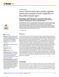
the framework to two common problems in cognitive radio: capacity maximization and dynamic spectrum access. Section two describes the cognitive radio architecture and discusses the reasoning and learning engines. Section three describes applications and how they work with the described model. Section four outlines our cognitive radio implementation. Section five concludes. II. C OGNITIVE R ADIO A RCHITECTURE A software radio (SR) can be defined as a radio implemented with generic hardware that can be programmed to transmit and receive a variety of waveforms. Cognitive radio is often thought of as an extension to software radio, and here we treat it as such. A cognitive radio extends a software radio by adding an independent cognitive engine, composed of a knowledge-base, reasoning engine, and a learning engine, to drive software modifications. A well-defined API dictates communication between the cognitive engine and the SR. Figure 1 illustrates this architecture and the interaction between various components. At any given time, the cognitive engine generates conclusions based on information defined in the knowledge-base, the radio’s long-term memory. These conclusions are the result of extrapolations of this information based on reasoning or learning. The reasoning engine is what is often referred to in AI literature as an expert system. The learning engine is responsible for manipulating the knowledge-base from experience. As lessons are learned, the learning engine stores them in the knowledge-base for future reference by the reasoning engine. Depending on the application, the learning engine may only be run to train a newly initialized radio, or it could be run periodically as the radio operates. The following sections describe each of the two engines in more detail. A. Reasoning and Planning The SR exports variables that are either read-only or readwrite. The read-only parameters represent statistics maintained by the SR, such as signal to noise ratio or bit error rate. The read-write variables represent configurable parameters such as transmit power, coding rate, or symbol constellation. These radio parameters are bound to predicates in the knowledge-base. Knowledge bases are very common in AI planning. The one we describe here contains two basic data structures. The first is a logic expression made up of predicates

2

Fig. 1.

Cognitive radio architecture showing the interactions between the software radio, knowledge-base, and policy and learning engines.

that represents the state of the environment. Predicates are expressions in first-order logic that evaluate to either true or false. The second set of data contained within the knowledgebase is actions. Actions define operations the reasoning engine could perform to change the state of its environment. Actions consist of a set of preconditions and postconditions. Preconditions must be inferable from the knowledge-base and evaluate true for the action to be selected. An action’s postconditions describe the modified state of the knowledge-base. To better illustrate the discussion, consider the following example, the objective of which is to decrease the modulation rate with a decrease in SNR. The knowledge-base contains the following predicates1 modRate(QP SK) ∧ snr(5 dB)

(1)

and the following action action : decreaseModulationRate precond : modRate(QP SK) ∧ snr(≤ 8 dB) (2) postcond : ¬modRate(QP SK) ∧ modRate(BP SK) The reasoning engine uses planning, which is a field of AI that works with logic2 . At any given time, it looks at the current state and determines which actions are executable in that state. All the possible resulting states are then evaluated to see which is optimal, where optimality is determined by an objective function fR (·). In our current example, we can successfully infer the preconditions from our knowledge-base. As a result, the decreaseModulationRate action is executed and the postcondi1 Note the commonly used notation in predicate calculus is as follows: logical AND is ∧, logical OR is ∨, and logical NOT is ¬. 2 We mostly consider scenarios that use forward chaining rather than backward chaining for inferencing, since we often don’t have a particular goal state.

tions are applied to the knowledge-base, resulting in KB 0 = KB ∧ postcond = (modRate(QP SK) ∧ snr(5 dB))∧ (¬modRate(QP SK) ∧ modRate(BP SK)) = modRate(BP SK) ∧ snr(5 dB)

(3)

Observe how modulation was changed from QPSK to BPSK when the SNR drops below 8 dB. While this example may seem elementary, it provides the fundamentals for reasoning in our cognitive radio. This example also illustrates the necessity for a learning engine. In complex radios with many inputs and many outputs, a countless number of actions would be necessary to account for all possible radio states. Rather than pre-programming this list of actions, the learning engine should auto-generate these actions based on experience. B. Learning The learning engine is responsible for augmenting the list of actions available to the radio that allow it to adapt to a changing environment. Many different learning algorithms are available to a cognitive radio, including hidden Markov models [3], neural networks [4], and genetic algorithms [5]. Nearly every learning technique involves the use of an objective function to determine the value of the learned data. In a cognitive radio, these objective functions reflect the overall goal of the application, such as maximizing channel capacity. The goal of the learning engine is to determine which input state will optimize the objective function. However, unlike the objective function used by the reasoning engine, there is no simple mathematical relationship between the system inputs and the objective function. In order for learning to be necessary, the precise effects of the changing inputs on the outputs must not be known. This is often the case in non-ideal radio channels. For example, we typically know that decreasing coding rate will also decrease bit error rate, but we don’t necessarily know by how much for an arbitrary communications channel. Using a learning engine, we can estimate our channel statistics and then using that data

3

we can make decisions that are optimal for our current RF environment. More formally, we define the radio’s state-space S. A particular state s ∈ S is made up of both the radio’s input predicates i and output predicates o. That is, s = i ∧ o. We have an objective function fL : S 7→ R that can be evaluated on a particular state s ∈ S and returns a real number. State s1 is preferable to state s2 if fL (s1 ) > fL (s2 ). The learning algorithm will try to precisely characterize fL (·) in an effort to find an optimal state. For example, a neural network using unsupervised learning could try to find statistical correlations between inputs and outputs to come up with a mathematical representation of fL (·). Similarly, evolutionary techniques such as genetic algorithms could evolve the radio’s state in order to maximize the objective function. After each state change, the resulting state will be evaluated. This process continues until a globally optimal state is found. Let’s assume that the learning algorithm evaluated N different inputs i1 , i2 , ..., iN with resulting outputs o1 , o2 , ..., oN before finding the optimal one. This implies that fL (iN ∧ oN ) ≥ fL (in ∧ on )

∀1 ≤ n ≤ N − 1

(4)

Thus we now know that if our radio is ever in state i1 ∧ o1 , ..., iN −1 ∧ oN −1 the optimal behavior is to set the radio inputs to iN . This equates to our learning engine generating the following actions for the policy engine: action : learnedActionX precond : ∀n ≤ N − 1 : in ∧ on postcond : ¬in ∧ iN

(5)

If the radio environment changes, however, oN may not result from iN , and iN may no longer be optimal. If this occurs, the learning engine should be aware of the changes and remove the suboptimal learned action from the knowledgebase. This can be expressed as: action : unlearnActionX precond : iN ∧ ¬oN

(6)

postcond : ¬learnedActionX The cognitive process, both reasoning and learning, is then reinstatiated in search of a new optimal state. The next section describes concrete instantiations of the policy and learning engines for particular applications. III. A PPLICATIONS In this section we describe several applications of learning to real radio problems. For each application, the inputs and outputs of the software radio are defined, along with an objective function. We then describe strategies for how a cognitive radio can solve the problem. All the applications assume the basic communications architecture shown in Fig. 2. This architecture defines a simplex link between a source and a destination software radio. The source radio has a cognitive engine that controls the source radio’s parameters, and uses the existing link to exchange

configuration information (e.g. modulation scheme, frequency, or bandwidth) and statistics (e.g. noise power or bit error rate). In order for this system to work, we must assume both the master and slave radio start off with the same initial configuration c0 . When the cognitive radio decides a change to configuration ci+1 is necessary, the master software radio sends a message containing ci+1 to the slave using configuration ci . A simple example of this would be a frequency hopping radio system where a hop to frequency fi+1 is signaled by sending a control message at frequency fi . To extend this basic architecture to a duplex link between two software radios, a cognitive radio engine can be added to the second radio. However, here we assume each cognitive engine acts as an independent agent controlling only outbound data and not communicating with other cognitive radio engines. To extend this model to a multi-party or ad-hoc network, each radio would maintain independent state in its cognitive radio engine for each destination node, as each pairwise, directed communications channel could have different properties. Certainly these channels are not completely independent, so some shared state can be used to more quickly find optimal solutions. A. Capacity Maximization in an AWGN Channel One very typical application of cognitive radio is to create a radio that can adapt to a channel to maximize its overall performance. Here we assume a fixed power, frequency, and bandwidth, since these parameters are more commonly thought of as being within the realm of dynamic spectrum access, detailed in Section III-C. Thus here we try to select a modulation type and coding rate to maximize capacity. For an AWGN channel, we can compute channel capacity using the Shannon-Hartley law [6], and our goal is to find a modulation type and coding rate that can get us as close to capacity as possible. Let us assume we have M modulation types M1 , M2 , ..., MM and N coding types C1 , C2 , ..., CN . Modulation type Mi can transmit di data bits per symbol and has a probability of bit error ei (S) for signal to noise ratio S. Coding type Cj has rate rj and can correct cj bit errors per block of size bj bits. For this application we assume an AWGN channel, and therefore ei (S) can be computed directly [6]. Our goal is to maximize capacity, so our objective function should reflect the capacity of our channel. For an arbitrary input configuration Mi ∧ Cj , we can compute channel capacity Ci,j by computing the raw data rate multiplied by the probability of not receiving cj + 1 or more bit errors. This results in a suitable objective function fR (·). Thus our goal is to find values Mi and Cj that maximize the objective function subject to our environment’s signal to noise ratio S. A key thing to notice here is that our radio output predicate snr(S) is independent of our inputs, and as a result, a pure policy-based radio can be used. The learning engine is not necessary. Given the above-defined objective function, the

4

Fig. 2.

Configuration of a basic simplex cognitive radio communications link

cognitive radio’s reasoning engine can determine the optimal radio operating parameters. A knowledge-base for maximizing channel capacity can be composed with several basic actions. The first can be used to set the modulation type. action : switchModType(A, B) precond : modT ype(A)

(7)

postcond : ¬modT ype(A) ∧ modT ype(B) The second can be used to set the coding type. action : switchCodeType(A, B) precond : codeT ype(A) postcond : ¬codeT ype(A) ∧ codeT ype(B)

(8)

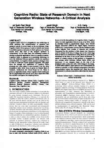
The reasoning engine will start with the initial state and derive all possible resulting states achievable with the above two actions. For all resulting states, the objective function will be evaluated, and the radio will then execute the actions that lead to that state. In this section, our key assumption was an AWGN channel where ei (S) can be derived for every possible modulation scheme. In the next section we look at a channel where ei (S) is not known, and learning algorithms must be used. B. Capacity Maximization in a non-AWGN Channel In the previous section we examined the problem of capacity maximization for an AWGN channel. We demonstrated that a cognitive radio can perform this without using a learning engine since the radio outputs were independent of the radio inputs. In this section, we consider a non-AWGN channel with fading, non-Gaussian noise, and interference. In this channel, we cannot know how any given modulation and coding scheme will perform without first trying it. In order to avoid a brute-force search, we must assume a continuous, convex solution space. To achieve this, there is a logical ordering of modulation types and coding types that results in a continuous, convex objective function, such that if we evaluate the objective function for modulation type Mi and find it to be less than Mi+1 , then the objective function evaluated for Mi−1 must be less than Mi . This will allow the use of an algorithm that performs a gradient search to find the objective function maxima. If the solution space is not continuous and convex it does not mean

Fig. 3. Sample objective function for a particular RF environment, showing optimality over modulation type 22m -QAM and coding rates from 0 to 1, interpolated onto a continuous surface.

we cannot find a solution, only that we cannot find it as quickly. In this application, our objective function will be heavily dependent on our outputs. Assuming our slave software radio can measure the corrected bit-success rate coming out of the decoder, the resulting capacity is the product of our bit-success rate, coding rate, and raw modulation data rate. As before, we can use this as our objective function fL (·). As an example, a sample objective function has been plotted in Fig. 3 for various modulation types and coding rates. Since it’s convex, hill climbing will efficiently yield an optimal configuration. C. Dynamic Spectrum Access Dynamic Spectrum Access (DSA) involves locating frequency bands and times when which a cognitive radio can transmit without causing harmful interference to other transceivers [7]. For example, consider a cognitive radio network operating in the UHF television bands, where transmission is permissible provided devices can guarantee they will not interfere with licensed broadcasts. More concretely, the goal is to locate center frequencies, bandwidths, and times when which a cognitive radio can transmit, while maximizing capacity and minimizing interference. This type of problem is very different from capacity maximization where we wanted to learn how our radio inputs affected our radio outputs. DSA involves learning where and when other radios will be transmitting.

5

If we assume all signals with which we are trying to coexist are continuous in time, the problem simplifies to one solvable by a policy-based radio. Imagine our SR exports predicates to the knowledge-base regarding detected signals s1 , s2 , ..., sN that are of the form signalF req(si , fi ) ∧ signalBW (si , Wi )

(9)

Our goal is to find some fc and W that does not overlap any detected signal, while maximizing W and consequently the radio’s capacity. First, let’s assume we have a helper function notOverlap(fc , W, si ) that evaluates to true if the band occupied by a signal centered at fc with bandwidth W does not overlap signal si . Then we can define our predicate action : moveBand(fold , Wold , fnew , Wnew ) precond : ∀i ≤ N : notOverlap(fnew , Wnew , si )

Fig. 4. Example showing cognitive radio coexisting with bursty signals in both frequency and in time.

(centerF req(fold ) ∧ bandwidth(Wold )) postcond : ¬(centerF req(fold ) ∧ bandwidth(Wold ))

Capacity vs SNR 1000

∧ (centerF req(fnew ) ∧ bandwidth(Wnew )) (10)

900

Capacity (kbps)

800

Then we define our objective function fR (centerF req(fc ) ∧ bandwidth(W )) = W

(11)

We now have a policy-based cognitive radio that will search out the largest continuous piece of bandwidth for communication. In more complex noise and interference environments, this approach is too simplistic, as different frequency bands may have different noise floors. Extension to this environment will require the use of a learning engine. Imagine our software radio exports predicate snr(S) for the currently-tuned center frequency and bandwidth. This gives us more information and we can define a better objective function based on the Shannon-Hartley law. fL (centerF req(fc ) ∧ bandwidth(W ) ∧ snr(S)) = W log2 (1 + S)

(12)

This learning objective function can only be evaluated when S is known, and this can only be computed after the radio has been tuned to center frequency fc . Another interesting extension to this idea is to consider noncontinuous signals, such as ones using time-division multiple access. For these situations, we can not only coexist in frequency but also in time. Using various cyclostationary statistical learning algorithms [8] we can compute the expected length of channel vacancy and incorporate that into our decision making. Imagine a neural network has computed for us the probability Pi (t) that signal si is transmitting at time t, where the probability is periodic over time τi . Our learning engine can then export to the knowledge-base predicates describing this signal. signalF req(si , fi ) ∧ signalBW (si , Wi ) ∧ (∀t < τ, Pi (t) > α : signalON (si , t) ∧ (∀t < τ, Pi (t) < α : signalOF F (si , t)

(13)

700 600 500 400 300 200 100 0 0

0.2

0.4

0.6

0.8

1

1.2

1.4

SNR (dB) Measured

Fig. 5. ratio

Capacity

Theoretical and achieved capacity as a function of signal to noise

A threshold α is used to indicate that the signal is present with very low probability. We can now extend our notOverlap function to take into consideration whether si is transmitting at time t, and our radio can compute its optimal course of action action : moveBand(fold , Wold , fnew , Wnew ) precond : ∀i ≤ N : notOverlap(fnew , Wnew , si , t) postcond : ¬(centerF req(fold ) ∧ bandwidth(Wold )) ∧ (centerF req(fnew ) ∧ bandwidth(Wnew )) (14) We can use the same objective function as before, or incorperate SNR if necessary. IV. I MPLEMENTATION To build upon the ideas developed in this paper, we have implemented a cognitive radio based on a generic cognitive engine [10]. It combines OSSIE, which is an open-source Software Communications Architecture (SCA) core framework implementation from Virginia Tech with the Soar cognitive engine from the University of Michigan. Within it we have implemented both the policy-based capacity maximization and the learning-based capacity maximization. The radio achieves the optimal configuration of

6

modulation and coding in an environment with time-varying noise power (see Figure 5). One of the biggest factors to consider in an implementation is adaptation time. The more “intelligence” you put behind the decision making process, generally the slower it is. If your cognitive engine is constantly running, searching for better radio configurations, it can utilize a significant portion of your processor time. Our policy radio adapts on the order of 10s of milliseconds, while our learning radio adapts on the order of 100s of milliseconds. We are currently working to implement dynamic spectrum access and adaptation to interference and fading channels within OSCR. V. C ONCLUSION Since the introduction of cognitive radio in 1999 [9], there have been many high-level discussions on proposed capabilities of cognitive radios. In this article, we have tried to formalize some of the architecture behind these ideas and the applications for which they are most suited, and give some insight into the differences between reasoning and learning. Certainly there is a great deal of future work in the field of cognitive radio, and in particular applications of machine learning to cognitive radio. The architecture described here is flexible enough to address many different applications provided they can be expressed in predicates, actions, and objective functions. The real work will be mapping potential applications to predicate calculus. R EFERENCES [1] IEEE 802.11, “Working group on wireless local area networks.” http://www.ieee802.org/11/. [2] T. Rondeau, C. Rieser, B. Le, and C. Bostian, “Cognitive radios with genetic algorithms: Intelligent control of software defined radios,” SDR Forum Conference 2004. [3] L. Rabiner, “A tutorial on hidden markov models and selected applications in speech recognition,” Proceedings of the IEEE, 1989. [4] S. Haykin, Neural Networks: A Comprehensive Foundation. Prentice Hall, 1998. [5] D. Goldberg, Genetic Algorithms in Search, Optimization, and Machine Learning. Addison Wesley, 1989. [6] J. Wozencraft and I. Jacobs, Principles of Communication Engineering. Waveland Press, 1990. [7] P. Leaves, S. Ghaheri-Niri, R. Tafazolli, L. Christodoulides, T. Sammur, W. Stahl, and J. Huschke, “Dynamic spectrum allocation in a multiradio environment: Concept and algorithm,” Conference on 3G Mobile Communication Technologies 2001. [8] T. Clancy and B. Walker, “Predictive dynamic spectrum access,” SDR Forum Conference 2006. [9] J. Mitola, “Cognitive radio: An integrated agent architecture for software defined radio.” Ph.D. Dissertation, KTH, 2000. [10] E. Stuntebeck, T. O’Shea, J. Hecker, and T. Clancy, “Architecture for an open-source cognitive radio,” SDR Forum Conference 2006.