Applied Engineering Using Schumann Resonance for ... - MDPI

applied sciences Article

Applied Engineering Using Schumann Resonance for Earthquakes Monitoring Jose A. Gazquez 1,2 , Rosa M. Garcia 1,2 , Nuria N. Castellano 1,2 ID , Manuel Fernandez-Ros 1,2 Alberto-Jesus Perea-Moreno 3 ID and Francisco Manzano-Agugliaro 1, * ID 1 2 3

*

ID

,

Department Engineering, University of Almeria, CEIA3, 04120 Almeria, Spain; [email protected] (J.A.G.); [email protected] (R.M.G.); [email protected] (N.N.C.); [email protected] (M.F.-R.) Research Group of Electronic Communications and Telemedicine TIC-019, 04120 Almeria, Spain Department of Applied Physics, University of Cordoba, CEIA3, Campus de Rabanales, 14071 Córdoba, Spain; [email protected] Correspondence: [email protected]; Tel.: +34-950-015396; Fax: +34-950-015491

Received: 14 September 2017; Accepted: 25 October 2017; Published: 27 October 2017

Abstract: For populations that may be affected, the risks of earthquakes and tsunamis are a major concern worldwide. Therefore, early detection of an event of this type in good time is of the highest priority. The observatories that are capable of detecting Extremely Low Frequency (ELF) waves ( 8.0) are usually generated whenever extensive areas of the subduction megathrust face a rupture [1]. There are examples of earthquake-produced tsunamis in the 2004 Sumatra earthquake (M-9.0) [2], accounting for 220,000 casualties, or in 2006, with the tsunami that developed from the Java earthquake (M-7.8) [3]. The intensity and destruction capacity of earthquakes and tsunamis are estimated by considering the area of vertical uplift of the sea bed, and these magnitudes are related to the geometry of the slipping fault when the earthquake rupture is located near the sea floor [4]. Seismic events produce variations in the magnetic field as well; the study of electromagnetic phenomena precursory of earthquakes and volcanic eruptions has been a very active subject during the last years [5]. Examples of this being the observation of Ultra Low Frequency (ULF) anomalies (300 Hz–3000 Hz) prior to the development of the Loma Prieta earthquake in 1989 near San Francisco [6,7]; later a geomagnetic field variation of 7.2 nT was detected approximately 7 min before the Tohoku earthquake occurred in 2011 and detected by the Iwaki observatory, at 210 km from the epicenter [8–10]. Another example is the possible detection of a series of pre-earthquakes magnetic anomalies that occurred on 25 April 2015, with epicentre in Nepal and a 7.8 magnitude. Detection was possible through the use of the Swarm magnetic satellites [11]. Appl. Sci. 2017, 7, 1113; doi:10.3390/app7111113

www.mdpi.com/journal/applsci

Appl. Sci. 2017, 7, 1113

2 of 19

In addition, after the Fukushima Daiichi nuclear plant disaster and the Great East Japan Earthquake Tsunami, which occurred in 11 March 2011, the requirement of cover human-environment symbiotic points is very important [12]. Tsunamis also have a major impact on economic aspects. After a tsunami occurs the flooding of the surrounding lands by seawater is common, damaging those lands and destroying plot borders. This causes damage to property rights and to the land administration system in general [13]. Therefore, after a Tsunami, it is necessary to re-establish the property lines again, using Global Positioning System (GPS) normally, as was the case in Indonesia [14]. From a geodesic point of view, it is well known that the definitive displacement of the zones near the epicentre is the results of earthquakes [15], e.g., the postseismic deformation after 2008 Wencham earthquake in China [16], or postseismic changes in Thai geodetic network owing to the Sumatra-Andaman mega-thrust earthquake in 2004 [17] and the Nias earthquake in 2005 [18]. Mega-splay faults are caused when very extensive thrust faults rising from the plate frontier megathrust intersects the seafloor along the lower earring of the margin. It has been hypothesized that these mega-splay faults transfer displacement efficiently to the near surface, contributing to the genesis of seismic phenomena. Recently, these facts have been identified as first order characteristics in the Nankai Trough [19], and are usual in other subduction areas such as Alaska [20], Sunda [21], and Colombia [22]. To understand the development of tsunamis during the formation of large earthquakes, it is necessary to determine the exact location of the slip of the decomposition system, called splay-frontal [23]. Instrumental measurements of earthquake and tsunamis largely come from tide seismological and gauge observatories and lately, bottom pressure recorders located in the deep ocean. The first time that the satellites Jason-1 and Topex-Poseidon collected transects of sea-height data using radar altimeter was in the 2004 Indian Ocean tsunami. These data showed a tsunami signal during the across the Indian Ocean [24]. The number of publications based on earthquake monitoring increases significantly and becomes a topic of increasing interest in the last decade [25,26]. Some authors suggest that a probabilistic approach might be a method for assessing the risk posed by seismic phenomena for a wide range of magnitudes [27]. Due to the relationship between earthquakes and tsunamis, both the recurrence allocation of events in time and the delivery of earthquake or landslide sizes can be used to calculate the tsunami probability. In coastal locations with a broad register of tsunami is the distribution scope that is similar to the ones from other natural damage such as landslides, forest fires, and earthquakes [1], which could be described as a power law [28]. But apart from this approach, methods for early detection are needed. Sensors can collect data to detect seismic phenomena that can lead to major natural disasters by means of a suitable seismic system and a correct treatment of the information. In addition, these systems could help with the early detection of a disaster, supporting the decisions to minimize human and environmental damage [12]. In the literature there are several types of sensor systems that measure different environmental responses after an earthquake and could determine the material damage caused. An example is the sensor Structural Health Monitoring (SHM), which measures the acceleration of the response movement of a building after an earthquake [29]; other sensors measure post-seismic deformations in horizontal structures [30] or in vertical structures [31]. Early detection of this type of seismic events can help save many lives. One such method of early detection could be the presence of ELF wave’s observatories, because of the relationship between Very Low Frequency/Extremely Low Frequency (VLF/ELF) waves and seismic phenomena [32,33]. During the eruption of the in the Kelud volcano eruption, seismic signals showing peaks at 3.7 mHz, 4.8 mHz, 5.7 mHz, and 6.8 mHz were observed in Indonesia. This fact suggests that an ionosphere-atmosphere coupling phenomenon was present along with the lithosphere-atmosphere coupling [34]. In addition, mentioning that such electromagnetic phenomena might be used to predict earthquakes, an example of this is shown in the precursors of the Loma-Prieta earthquake [35], or for the Great East Japan earthquake of 2011 (or Tohoku earthquake) [36].

Appl. Sci. 2017, 7, 1113

3 of 19

The aim of this paper is to represent the major worldwide earthquakes and tsunamis of twentieth and twenty-first centuries, and to show the location of ELF wave’s observatories existing in the world accounting for the relationship between the two phenomena. This allows us to visualize the zones high probability of seismic phenomena. Taking into consideration the presence of seismic phenomena and their possible detection, different areas of the world will be shown which are suited to this kind of observatories. 2. Materials and Methods 2.1. Seismic Phenomena and ELF Waves The importance of the study of precursors or indicators of seismic activity is a key to early detecting and preventing succession of major disasters [37]. Seismic events can be related to different types of events. There is evidence indicating that a link between the lithosphere-atmosphere-ionosphere occurs before the occurrence of seismic events [38]. Understanding these processes’ physics and possibility of it being used to develop an early detection system is the subject of great research and development in recent decades. It has demonstrated the influence of seismic events on this type of ELF signals, setting both types of signals artificially and analyzing the behavior of electromagnetic waves when they are motivated by earthquakes [32]. One of the first attempts to standardize ELF wave monitoring on a global scale dates back to 1985, thus it is considered a fairly developed work topic in recent years [39]. Also, there exist other publications that detect anomalies in signals produced by the seismic phenomenon. One example is the correlation between the seismic phenomena and the Outgoing Long-wave Radiation (OLR) data. These signals can be observed by satellites [16], such as the case of the Chinese Earthquake (Wenchuan and Lushan earthquakes) that occurred between 2006 and 2013. The detection of such anomalies can also be carried out by observatories or ELF/VLF stations [33]. These observatories are located in very low-noise locations. In them, the ELF/VLF range (signals up to 300 Hz) and the orthogonal components of the magnetic field (Bx , By and Bz ) can be measured. Three orthogonal induction coil magnetometers are normally employed. The Bx component usually represents the North-South (NS) geomagnetic component of the magnetic field. It can be determined by the induction magnetometer whose axis is aligned with the direction NS, so that the component Bx is sensitive to waves propagating in the East-West (EW) direction. The other component of interest is the By component that is sensitive to waves propagating in the meridian plane [40]. ELF/VLF signals propagate through the environment, and are detected by an appropriately located ELF/VLF receiver over a zone where enhanced radio emissions are happening prior to a great earthquake. Some studies about ionosphere-atmosphere-groundwater phenomena great earthquakes (M > 6.5) associate this occurrence with strong ELF noises or anomalies present in signals located in the ELF frequency band [41]. One of the most important ELF signals, which are affected by the presence of these seismic events is the Schumann Resonance (SR) [42]. These resonances are produced by natural phenomena; they were predicted theoretically in the 50’s, but no graphical representation of them was established until 1962 [43]. The SR signals are very weak signals, on the order of PicoTesla, and occur in the space between the earth and the ionosphere, as indicated in Figure 1. This space acts as a resonant cavity or waveguide for these signals, since it has a finite or limited size [44].

Appl. Sci. 2017, 7, 1113 Appl. Sci. 2017, 7, 1113

4 of 19 4 of 20

Figure 1. Phenomenon of Schumann Resonance. Figure 1. Phenomenon of Schumann Resonance.

The measurement of these signals allows developing various applications. This includes In regards to the relationship between the mean of these phenomena ELF and the existence of determining the global lightning activity or storms by diurnal variations in the amplitude of the seismic events, there are relatively recent works showing the appearance of abnormal variations in signal continuous records [45], or the study of planetary electromagnetic environment [46]. Another the amplitude and phase of these ELF signals when crossing regions of certain seismic activity. These application of SR signals that has aroused great interest in recent years is as a global tropical changes are due to displacement of the inner boundary of the ionosphere in a few kilometers when thermometer. Since a frequency shift of resonance peaks has been observed related to the global seismic activity occurs [48]. temperature increase of the planet or global warming [47]. Other publications have shown the fact of the signals derived from this phenomenon in a period In regards to the relationship between the mean of these phenomena ELF and the existence of in which large earthquakes occurred, such as the case developed and understood in Taiwan between seismic events, there are relatively recent works showing the appearance of abnormal variations in 1999 and 2004. It is noted that earthquakes produce a variation of about 1 Hz in the localization of the amplitude and phase of these ELF signals when crossing regions of certain seismic activity. These the peak frequency. Another anomaly that is detected in this type of work is an atypical amplitude changes are due to displacement of the inner boundary of the ionosphere in a few kilometers when increase of all its modes, highlighting the variation in the fourth mode of resonance, as observed in seismic activity occurs [48]. large earthquakes M > 6 [49]. Other publications indicate that the monitoring this signal allows the Other publications have shown the fact of the signals derived from this phenomenon in a period checking of the existence of depressions in the frequency of the fourth mode resonance occurring in which large earthquakes occurred, such as the case developed and understood in Taiwan between between two and six days before one of the study earthquakes [50]. In most of the works, variations 1999 and 2004. It is noted that earthquakes produce a variation of about 1 Hz in the localization of or anomalies in these signals can be observed with days or even weeks in advance before the the peak frequency. Another anomaly that is detected in this type of work is an atypical amplitude occurrence of any earthquake. For example, variations have been detected three weeks before the increase of all its modes, highlighting the variation in the fourth mode of resonance, as observed in earthquake that happened on the 11 of March 2011, with an 8.9 magnitude in front of the Japanese large earthquakes M > 6 [49]. Other publications indicate that the monitoring this signal allows the coast [51]. Signals anomalies were detected for few days, as well ahead before the Sichuan earthquake checking of the existence of depressions in the frequency of the fourth mode resonance occurring that took place with a magnitude of 8.0 [52], and the Kobe earthquake of 6.0 magnitude in 2013 [53]. between two and six days before one of the study earthquakes [50]. In most of the works, variations or Therefore, the study and analysis of these signals ELF may be a method for detecting seismic anomalies in these signals can be observed with days or even weeks in advance before the occurrence events. The presence of ELF stations or observatories in regions with seismic activity or nearby is of any earthquake. For example, variations have been detected three weeks before the earthquake that useful, so that detection is more effective, despite the resonance phenomenon being a global one. happened on the 11 of March 2011, with an 8.9 magnitude in front of the Japanese coast [51]. Signals anomalies were detected for few days, as well ahead before the Sichuan earthquake that took place ELF Sensor with a magnitude of 8.0 [52], and the Kobe earthquake of 6.0 magnitude in 2013 [53]. ELF sensors built byanalysis combining vertical electric field be sensors and for horizontal Therefore, theare study and of these signals ELF may a method detectingmagnetic seismic induction coils [54]. This process is very complex due to the large number of factors involved, such events. The presence of ELF stations or observatories in regions with seismic activity or nearby is as its low frequency, theisweakness of the signal be resonance detected, the non-uniformity ionosphere, useful, so that detection more effective, despitetothe phenomenon beingofa the global one. the manifestation of natural electromagnetic noise, and the interference caused by industrial zones, ELF Sensor as background noise in the process [55]. These are some of the reasons behind the small appearing number ELF sensors to other observatories; although has magnetic increased ELF of sensors are builtcompared by combining vertical electric field sensorsthat andnumber horizontal fourfold since the five observatories accounted for in 1999. induction coils [54]. This process is very complex due to the large number of factors involved, such observatories are located throughout thedetected, world. However, the largestofconcentration of as its These low frequency, the weakness of the signal to be the non-uniformity the ionosphere, such observatories is in Japan, where the occurrence of seismic events is greater [56]. Many of these the manifestation of natural electromagnetic noise, and the interference caused by industrial zones, observatories are attempting to establish a correlation between the ELF signals measured and seismic activity, and to compare with data from other stations. For this, a correlation is established within the

Appl. Sci. 2017, 7, 1113

5 of 19

appearing as background noise in the process [55]. These are some of the reasons behind the small number of ELF sensors compared to other observatories; although that number has increased fourfold since the five observatories accounted for in 1999. These observatories are located throughout the world. However, the largest concentration of such observatories is in Japan, where the occurrence of seismic events is greater [56]. Many of these observatories are attempting to establish a correlation between the ELF signals measured and seismic Appl. Sci. 2017, 7, 1113 5 of 20 activity, and to compare with data from other stations. For this, a correlation is established within the different components of the magnetic field [57],and andthe thedevelopment developmentof of theoretical theoretical models models for different components of the magnetic field [57], for describing the intensity of the SR by disturbances in the ionosphere over the top of the epicenter describing the intensity of the SR by disturbances in the ionosphere over the top of the epicenter of of an an earthquake. earthquake. One One of of these these theoretical theoretical models models is is based based on on ionosphere’s ionosphere’s vertical vertical conductivity conductivity profile profile model, cavity. The possible disturbance is introduced withwith the model, describing describingthe theregular regularEarth-ionosphere Earth-ionosphere cavity. The possible disturbance is introduced modified model. The localized ionosphere modification shows a Gaussian radial dependence; it has a the modified model. The localized ionosphere modification shows a Gaussian radial dependence; it 1-Mm radius, with the decrease reaching 20 km in the lower ionosphere height over the epicenter of the has a 1-Mm radius, with the decrease reaching 20 km in the lower ionosphere height over the earthquake Also, the diffraction problem in the Earth-ionosphere with a disturbance epicenter of(Taiwan). the earthquake (Taiwan). Also, the diffraction problem in thecavity Earth-ionosphere cavity can be resolved by using the Stratton-Chu integral equation [58]. with a disturbance can be resolved by using the Stratton-Chu integral equation [58]. One stations hashas been developed and steadily improved by theby research group TIC019 One of ofthese theseELF ELF stations been developed and steadily improved the research group of Almeria University and it is located in Calar Alto (Almeria, Spain), Figure 2. This observatory TIC019 of Almeria University and it is located in Calar Alto (Almeria, Spain), Figure 2.began This operation in 2011, the first observatory of first its kind in Spain. of its kind in Spain. observatory beganbeing operation in 2011, being the observatory

Figure 2. Calar Alto Extremely Low Frequency (ELF) Station (Spain). Figure 2. Calar Alto Extremely Low Frequency (ELF) Station (Spain).

The technology used in this type of observatories has evolved significantly in recent years. The Theaspects technology in this type observatories hasonly evolved significantly in recent years. general of it used are described in of a few papers, but a handful of articles explicitly setThe the general aspects of it are described in a few papers, but only a handful of articles explicitly set the methodology used to capture and measure ELF signals. Figure 3 shows the block diagram of Calar methodology used to capture and measure ELFdiagram signals.shows, Figure the 3 shows theconsists block diagram of stages Calar Alto ELF observatory (Almeria, Spain). As the system of a set of Alto ELF observatory (Almeria, Spain). As the diagram shows, the system consists of a set of stages from signal capture and local real-time processing to transmission to the University of Almeria and from signal capture and local real-time processing to transmission thestages University Almeria and the the insertion of post-processed data into an interactive database. to The of the of measuring system insertion of post-processed data into an interactive database. The stages of the measuring system are are as follows: as follows: (1) Signal Capture: formed by the ELF magnetic sensors. (1) Signalof Capture: formedof bysignal, the ELF magnetic sensors. (2) Stage conditioning: constituted by a high gain differential amplifier and a level (2) scaled Stage ofadapter. conditioning: of signal, constituted by a high gain differential amplifier a level Through this process a suitable signal is obtained at the input and of the nextscaled stage, adapter. Through this process a suitable signal is obtained at the input of the next stage, with a with a maximum dynamic range input and the lowest output clipping. A passband filter ranging maximum dynamic rangeincluded input and clipping. A passband ranging from 3 from 3 to 100 Hz is also in the thislowest stage. output This filter attenuates signalsfilter outside the desired band, preventing undesired intermodulation or cross-modulation phenomena. (3) The stage of the Analog/Digital converter (A/D converter): This stage has two channels, one for each sensor. It converts the analog signal into 24-bit samples per channel with a sample rate of 196 samples/s. (4) The last stage is the data transmission and storage. It is constituted by a local information storage

Appl. Sci. 2017, 7, 1113

6 of 19

to 100 Hz is also included in this stage. This filter attenuates signals outside the desired band, preventing undesired intermodulation or cross-modulation phenomena. (3) The stage of the Analog/Digital converter (A/D converter): This stage has two channels, one for each sensor. It converts the analog signal into 24-bit samples per channel with a sample rate of 196 samples/s. (4) The last stage is the data transmission and storage. It is constituted by a local information storage (data logger), which serves as failsafe from temporary interruptions in the transmission system. Additionally it allows data transmission from the A/D converter to the installations of the University of Almeria by means of a digital radio link. In such facilities, the data is inserted an interactive database for post-processing and study. Appl.into Sci. 2017, 7, 1113 6 of 20

Figure ELFwave wave sensor diagram. Figure 3. 3.ELF sensor diagram.

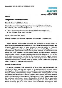
Themagnetic magneticsensors sensorsare aretwo twomagnetic magneticantennas antennasoriented orientedalong alongthe themain maincardinal cardinaldirections directions The (north-south and east-west). Each sensor is made up of two symmetrical coils that provide balanced (north-south and east-west). Each sensor is made up of two symmetrical coils that provide balanced differentialsignals signalshelping helpingtotoreduce reducecommon commonmode modeeffects effects[59,60]. [59,60].An Anoptional optionalnotch notchfilter filterwas was differential implemented as part of the measurement system using a double Active cell [61] to attenuate the implemented as part of the measurement system using a double Active cell [61] to attenuate the power signals. power signals. TheA/D A/D converter converter system system consists consists ofof aa24-bit 24-bithigh highresolution resolutionsystem systemthat thatisisbased basedonon The oversampling techniques. The obtained data from the converter is subject to a decimating process oversampling techniques. The obtained data from the converter is subject to a decimating process through temporary averaging. This causes a reduction in the acquisition noise, as well as the through temporary averaging. This causes a reduction in the acquisition noise, as well as ininthe sampling frequency. high-performance embedded Digital Signal Processor (DSP) system done sampling frequency. ByBy a ahigh-performance embedded Digital Signal Processor (DSP) system isisdone by this pre-processing. Ultimately, data are sent in real-time by a high-speed link to the research by this pre-processing. Ultimately, data are sent in real-time by a high-speed link to the research group facilities in Almeria University, is worked using PowerDensity Spectral Density (PSD) group facilities in Almeria University, where where is worked using Power Spectral (PSD) estimation estimation techniques [62].Through the development of this system, the Schumann resonance signal techniques [62]. Through the development of this system, the Schumann resonance signal capture capture efficiency will be enhanced, thereby facilitating their subsequent analysis The data efficiency will be enhanced, thereby facilitating their subsequent analysis and study. and The study. data collected collected these observatories are like those presented In athese figures, a from these from observatories are like those presented in Figure 4a,b.in InFigure these 4a,b. figures, periodogram periodogram and a spectrogram are represented, respectively, recorded from the Calar ELF and a spectrogram are represented, respectively, recorded from the Calar Alto ELF station Alto (Spain). station (Spain). These representations were established from the data recordings in normal conditions These representations were established from the data recordings in normal conditions of the day the day 162015. September 2015. The periodogram (Figure 4a) by was30obtained by 30 min the 16ofSeptember The periodogram (Figure 4a) was obtained min averaging, the averaging, result of Fast result of Fast Fourier Transform (FFT) of 20 s data segments. The 24 h spectrogram is composed from periodograms that are obtained by averaging each 10-min segments of 20 s. In this periodogram, the first 7 resonance peaks can be observed, as well as the signal from the power lines. In the spectrogram, you can see beside the Resonance Schumann modes, variations in power line signals and other signals that affect all frequencies about the 500 min, which is due to

Appl. Sci. 2017, 7, 1113

7 of 19

Fourier Transform (FFT) of 20 s data segments. The 24 h spectrogram is composed from periodograms 7 of 20 that are obtained by averaging each 10-min segments of 20 s.

Appl. Sci. 2017, 7, 1113

(a)

(b) Figure 4. Data from from the Calar (Spain): (Spain): (a) The 30 (b) The 24 h(b) The Figure 4. Data the Alto CalarSensor Alto Sensor (a)min Theperiodogram. 30 min periodogram. Spectrogram. 24 h Spectrogram.

2.2. Worldwide Map of ELF Observatories and Seismic Events In this periodogram, the first 7 resonance peaks can be observed, as well as the signal from the The number of stations or observatories ELFsee today is not large, due Schumann to many factors, among power lines. In the spectrogram, you can beside thetoo Resonance modes, variations which is the difficulty of the measurement process or the all study of such signals. study is an issue is due in power line signals and other signals that affect frequencies about This the 500 min, which thattoisstrong being widely years. ELF/VLF stationsoforthese observatories exist today can bewe can wind. developed Therefore,inbyrecent monitoring the evolution electromagnetic signals, classified into severaloftypes: establish a study their variation and find out the mechanisms that are related these changes with the occurrence of seismic events. To ELF signals’ alterations with strong several cases (a) Observatories that measure therelate disturbances caused by seismic activity onearthquakes, the ELF radiation, must be studied. The significance of the data would depend on the number of ELF stations around the considering subELF observatories. These subELF observatories usually record the possible epicenter, soincommon ELFmagnetic alterations could be some foundhave and very lay out criteria that might variations the Earth’s field, where lowthe frequencies (less thanallow 0.03 early earthquake detection. Hz). An example of this is the station of Uchimura (Japan), which allows for studying the data collected in the range comprised between 0.01 to 0.033 Hz frequencies [52]. In other publications, 2.2. of ELF Observatories and Seismic Events theWorldwide signals ofMap lower frequencies (0.01–0.02 Hz) are analyzed [54] to establish anomalies or unaccounted perturbations of the earth’s magnetic before the occurrence offactors, severalamong The number of stations or observatories ELF todayfield is not too large, due to many earthquakes of interest [53]. Considering the development of such stations of great interest which is the difficulty of the measurement process or the study of such signals. This study isfor an issue possible applications in the field of earlyyears. detection is considered emerging theme in the can be that is being widely developed in recent ELF/VLF stations as or an observatories exist today study. into several types: classified

Appl. Sci. 2017, 7, 1113

(a)

(b)

(c)

8 of 19

Observatories that measure the disturbances caused by seismic activity on the ELF radiation, considering subELF observatories. These subELF observatories usually record the possible variations in the Earth’s magnetic field, where some have very low frequencies (less than 0.03 Hz). An example of this is the station of Uchimura (Japan), which allows for studying the data collected in the range comprised between 0.01 to 0.033 Hz frequencies [52]. In other publications, the signals of lower frequencies (0.01–0.02 Hz) are analyzed [54] to establish anomalies or unaccounted perturbations of the earth’s magnetic field before the occurrence of several earthquakes of interest [53]. Considering the development of such stations of great interest for possible applications in the field of early detection is considered as an emerging theme in the study. Other observatories had recorded signals in the 1 Hz to 50/60 Hz spectrum. The latter are important frequencies due to the presence of strong interference signals in this band [63]. It might be interesting to consider the different sub-bands within this range [64]. There are also observatories that monitor the exact value of frequencies. Mainly, these values happen to be multiples of the principal frequency depending on the country. These frequencies are usually 223 Hz (in countries having 60 Hz as principal frequency) and 233 Hz (in countries having 50 Hz as principal frequency) [65]. Other observatories use a frequency of 17 Hz [66].

All of the observatories mentioned earlier measure signals of original nature, but there are other stations that monitor artificial signals that are generated by human activity, such as signals in the VLF band that are issued for the navigation aid [67]. Furthermore, not all of the stations have the same measuring devices. The most common are seismometers, acoustic meters, or telluric current meters. These instruments are of great importance to correlate the different parameters of interest with the detection of natural phenomena. The data above can be related to other meteorological data, such as wind speed, humidity, temperature, and atmospheric pressure [48]. Table 1 shows the World-Wide ELF/VLF observatories. This list is in descending order, showing the estimated station range according to the references listed in the table itself. The observatories with range above 1000 km are usually used for communications and shorter ranges are aimed for the detection of natural disasters. The station’s sensitivity range is the maximum distance at which it can detect an atmospheric phenomenon. Therefore, this range depends on the magnitude of the different phenomena it can detect. Table 1. Worldwide ELF (Extremely Low Frequency) Sensors. ID (Reference)

Name

Country

Lat (◦ N)

Long (◦ E)

Range (km)

Year

HAS-(ARC) [68] KS(R) [69] ES-(SW) [70] FS-(USA) [71] LS-(R) [72] GS-(R) [73] BS-(PO) [74] NS-(H) [75] MS-(J) [57] HYS-(PO [76] RIS(USA) [75] SS-(T) [77] CAS-(SP) [60] HS-(USA) [75] KO-(J) [78] TO-(J) [75] NO-(J) [48] US-(J) [78] ISO-(J) [79]

Hournsund Kola Esrange Fairbanks Letha Gakona Belsk Nagycenk Moshiri Hylaty R. Island Sorköy Calar Alto Hollister Kakioka Tottori Nakatsugawa Uchiura Ibaraki

Arctic Pole Russia Sweden USA Russia Russia Poland Hungry Japan Poland USA Turkey Spain USA Japan Japan Japan Japan Japan

77.8 68.8 67.9 64.8 64.4 62.7 51.8 47.6 44.4 42.2 41.7 40.8 37.1 36.8 36.2 35.5 35.4 35.1 34.8

20.7 34.5 21.0 −147.7 33.9 −143.9 20.7 16.7 142.2 22.5 −71.6 27.1 −2.6 −121.5 140.2 134.2 137.5 140.2 135.6

500 7500 500 4000 1000 5600 550 4400 6000 320 4466 500 500 1500 300 100 100 420 200

2000 1999 2000 1987 2007 2012 1999 2006 1998 1994 2007 2007 2012 1995 2006 1973 2000 2012 1999

Appl. Sci. 2017, 7, 1113

9 of 19

Table 1. Cont. ID (Reference)

Name

Country

Lat (◦ N)

Long (◦ E)

Range (km)

Year

OTS-(J) [49] KAO-(R) [50] NS-(IS) [75] MS-(MX) [80] AS-(IND) [81] BAS-(ANT) [82] SPS-(ANT) [75]

O. Tsushima Kamchatka Negev Mexico Allahabad Bellinshausen South Pole

Japan Russia Israel Mexico India Antarctic Pole Antarctic Pole

34.6 32.9 30.6 19.8 16.1 −62.2 −89.0

129.4 158.2 35.0 −101.7 81.7 −59.0 134.0

1000 50 660 500 4000 1625 4000

1998 2001 1998 2014 2007 2007 1997

In order to build the worldwide map of seismic events, records were used from the Significant Earthquake of National Oceanic and Atmospheric Administration (NOAA), containing Appl. Sci. 2017,Database 7, 1113 9 of 20 information on destructive earthquakes from 2150 B.C. to the present day. All of the featured earthquakes damage (at (atleast least11million milliondollars), dollars),1010oror earthquakesmeet meetatatleast leastone oneof ofthe thefollowing: following: Moderate Moderate damage more generated aa tsunami tsunami[78]. [78].More Morethan than morecasualties, casualties,Magnitude Magnitude 7.5 7.5 or or greater, greater, or or the the earthquake earthquake generated 1400earthquakes earthquakeshave havebeen beenrepresented representedin in this work, also 1400 also considering consideringthose thosewith withtsunami tsunamiassociated. associated. Theseparticular particular earthquakes accompanied tsunami occurrence were selected These earthquakes thatthat are are accompanied withwith tsunami occurrence were selected among among all others due to the fact that these events have produced huge disasters throughout the all others due to the fact that these events have produced huge disasters throughout the history. Thus, history. Thus,istheir detection is of great interest. The presentation of other earthquakes the map their detection of great interest. The presentation of other earthquakes in the map wouldinhave made have made much complex to read due of toseismic the highevents number seismic eventsin it would much complex andit difficult to read and due difficult to the high number thatofhave occurred that have occurred period of timeThey (thewouldn’t last two add centuries). wouldn’tasadd the considered periodin of the timeconsidered (the last two centuries). relevantThey information well, relevant information as well, since the seismic zones are still active. since the seismic zones are still active. Theprevious previousdata datawas waslaid laidout outover over aa map, map, displaying displaying recent The recent seismic seismicevents eventsofofinterest interestand andthe the stations indicated in Table 1, with their corresponding detection range (as set by relevant literature). stations indicated in Table 1, with their corresponding detection range (as set by relevant literature). Figure5 5shows showsthe thefinal finalresults. results. It It is is worth worth mentioning mentioning that Figure that annually, annually, there thereare areabout aboutone onemillion million earthquakes of M = 2.0 [83]. earthquakes of M = 2.0 [83].

Figure through ELF ELF Sensors. Sensors. Figure5.5.Tsunami Tsunami risk risk alerts alerts worldwide through

The WinkelTripel projection has been used to build the map. The name Tripel (German for “triple”) is a reference to Winkel’s goal of reducing three kinds of distortion: area, direction, and distance. The WinkelTripel has the smallest skewness, so it is suited for mapping the entire world [84]. Nowadays it is found that this projection has been used to show the location of earthquakes recorded all over the earth, mainly due to the good representation of highest latitudes. It is used from

Appl. Sci. 2017, 7, 1113

10 of 19

The WinkelTripel projection has been used to build the map. The name Tripel (German for “triple”) is a reference to Winkel’s goal of reducing three kinds of distortion: area, direction, and distance. The WinkelTripel has the smallest skewness, so it is suited for mapping the entire world [84]. Nowadays it is found that this projection has been used to show the location of earthquakes recorded all over the earth, mainly due to the good representation of highest latitudes. It is used from 1998 by the National Geographic Society for worldwide maps [85], replacing the Robinson projection as the standard projection. 3. Results and Discussion When considering Figure 5, we have developed several maps that are raised or propose new ELF sensors as stations to provide coverage to potentially vulnerable regions. Appl. Sci. 2017, 7, 1113 10 of 20 The label of “high seismic risk” could be tagged to the zones of Central America, Andes, the most oriental part of Europe, Philippines, Indonesia, and Japan, with the threeevents last regions having a high high occurrence of earthquakes and tsunami. There are frequent seismic of great magnitude occurrence of earthquakes and tsunami. There are frequent seismic events of great magnitude that that involve high damages: the Sumatra Tsunami in 2010 [18] or the Tsunami Japan 2011 [51], and involveThis highisdamages: thereasons Sumatra in 2010 [18] oranalysis the Tsunami Japan [51], and others. one of the forTsunami which the study and of this type2011 of event is ofothers. great This is one of the reasons for which the study and analysis of this type of event is of great importance importance for the population. Figure 6 shows the current ELF stations along with the ELF stations, forproposed the population. Figure 6 shows the current stations along with the ELF stations, as proposed as in Table 2. It can be observed thatELF in this figure the coverage of the areas with seismic in Table 2. It can be observed that in this figure the coverage of the areas with seismic risk is greater risk is greater than the one established in Figure 5, where there are only represented the existing ELF than the one established in Figure 5, where there are only represented the existing ELF stations. stations.

Figure 6. Tsunami risk alerts worldwide through proposed ELF observatories with a 1000 km of ratio. Figure 6. Tsunami risk alerts worldwide through proposed ELF observatories with a 1000 km of ratio.

Table 2. Proposed ELF Observatories (1000 km). ID AS-1 OC-1 AS-2 OC-2 SA-1 OC-3 SA-2 OC-4

Geographical area Asia—Basey (Western Samar)—Philippines Indonesia Asia—Dewakang (Liukang) Indonesia Oceania—Papua New Guinea South America—Peru Oceania—Malo Island (Vanuatu) South America—Chile Oceania—Tongatapu

Lat (°N) 11.416 −0.773 −5.490 −5.809 −5.979 −15.25 −20.811 −22.342

Lon (°E) 125.175 133.959 118.630 151.002 −78.942 166.83 −69.536 −176.206

Appl. Sci. 2017, 7, 1113

11 of 19

Table 2. Proposed ELF Observatories (1000 km). ID

Geographical Area

Lat (◦ N)

Lon (◦ E)

AS-1 OC-1 AS-2 OC-2 SA-1 OC-3 SA-2 OC-4 SA-3 OC-5

Asia—Basey (Western Samar)—Philippines Indonesia Asia—Dewakang (Liukang) Indonesia Oceania—Papua New Guinea South America—Peru Oceania—Malo Island (Vanuatu) South America—Chile Oceania—Tongatapu South America—Chile Oceania—New Zealand

11.416 −0.773 −5.490 −5.809 −5.979 −15.25 −20.811 −22.342 −37.724 −43.446

125.175 133.959 118.630 151.002 −78.942 166.83 −69.536 −176.206 −73.260 170.468

Table 2 proposes with a minimum of 10 new ELF observatories to cover the seismic risk of all these areas of the earth, with a standard range of 1000 km. With this range, all of the zones of interest Appl. Sci. 2017, 7, 1113 11 of 20 could have been covered. So, South America can be covered by three observatories that located in Chile and Peru, while Oceania needs five observatories, and the south of Asia needs at least two of them. If a smaller range is considered, the numbers of suggested stations should be higher, an example If a smaller range is considered, the numbers of suggested stations should be higher, an example shown in Figure 7. In this figure the data in Table 3, where possible ELF stations are established to shown in Figure 7. In this figure the data in Table 3, where possible ELF stations are established to cover the vulnerable areas seismic coverage with a radius of 500 km are represented. cover the vulnerable areas seismic coverage with a radius of 500 km are represented.

Figure 7. Tsunami risk alerts worldwide through proposed ELF observatories with a 500 km of radio. Figure 7. Tsunami risk alerts worldwide through proposed ELF observatories with a 500 km of radio.

Table 3. Proposed ELF Observatories (500 km). ID AS-1 AS-2 OC-1 OC-2 OC-3 OC-4 OC-5

Geographical Area Philippines Asia—Basey (Western Samar)—Philippines Indonesia Indonesia Oceania—Papua New Guinea Oceania—Papua New Guinea Indonesia

Lat (°N) 13.723 6.413 0.389 −0.808 −4.8817 −5.8344 −6.493

Lon (°E) 121.153 126.161 120.841 132.751 144.243 153.886 126.073

Appl. Sci. 2017, 7, 1113

12 of 19

Table 3. Proposed ELF Observatories (500 km). ID

Geographical Area

Lat (◦ N)

Lon (◦ E)

AS-1 AS-2 OC-1 OC-2 OC-3 OC-4 OC-5 OC-6 SA-2 OC-7 SA-3 OC-8 OC-9 SA-1 SA-4 SA-5 OC-10 OC-11 SA-6

Philippines Asia—Basey (Western Samar)—Philippines Indonesia Indonesia Oceania—Papua New Guinea Oceania—Papua New Guinea Indonesia Indonesia South America—Peru Oceania—Salomon Islands South America—Peru Oceania—Niue Oceania—Malo Island (Vanuatu) South America—Ecuador South America—Chile South America—Chile Oceania—Tonga Oceania—New Zealand South America—Chile

13.723 6.413 0.389 −0.808 −4.8817 −5.8344 −6.493 −8.569 −10.500 −11.127 −17.000 −18.027 −18.421 −22.185 −24.537 −33.235 −26.547 −41.25 −41.497

121.153 126.161 120.841 132.751 144.243 153.886 126.073 115.741 −77.000 162.771 −72.000 −170.00 168.411 −79.902 −70.707 −71.726 −180.00 175.00 −72.986

The minimum number of stations to be considered in this case is 19. So, South America can be covered by six observatories located in Chile, Peru, and Ecuador, while Oceania needs 11 observatories, and the south of Asia needs at least two of them. There is no theoretical model that establishes a specific range for the detection of this type of phenomena, and appointed error in these measures. The ranges described in Table 1 were estimated empirically according to the sensitivity of the phenomena captured, with usual distances of between 500 km and 1000 km. Consistent with these data, possible ELF stations with a range of 1000 km (Table 2) and 500 km (Table 3) have been proposed. The technology improvements allow for a greater sensitivity for the capture of these phenomena. Recently, the largest number of the ELF observatories resides in the region of Japan; they cover the major part of its territory. The rest of observatories are distributed on the North American coast and Europe most commonly in its oriental zone. In the Figure 5, it should be considered that the African continent has less seismic activity that can produce tsunami due to the localization of the tectonic plates, which makes it a stable zone. We can observe that there exist numerous zones in southern hemisphere, where the occurrence of seismic events is elevated. Currently, there are no ELF observatories in these zones, which make the prediction of seismic events possible and thus they are considered as vulnerable areas. So, in Africa, there is no evidence of significant seismic events recorded and therefore installing ELF observatories would not be a priority, although it would be recommended. However, there are other areas of the world with high earthquake intensity and risk to human life as consequence to the high population density [86]. The low atmospheric attenuation with some latitude dependence of ELF signals (with an average of 0.64 dB/km at 40 Hz) allows for wave propagations at global scale [87]. Despite the global character of these signals, the signals anomalies related to the occurrence of seismic events cannot be detected whenever the magnitude is less than 6 (M < 6). It should be considered that seismic phenomena of such magnitudes can also cause disasters and should be taken into account for their early detection [25]. This is one of the reasons behind the necessity of establishing new ELF stations in the potentially active regions, such as the Asian zone or the south of America. The development of new ELF stations in areas of frequent seismic activity could be considered as a very useful tool for the possible detection of seismic phenomena. There are researchers with great

Appl. Sci. 2017, 7, 1113

13 of 19

experience in the correlation of seismograms with previous anomalies of the natural patterns of ELF signals. The author Hayakawa M. is one of the main advocates of this theory, as indicated by the large number of articles he has developed in this topic, although the list of researchers is rather extensive. Table 4 shows some of the precursor phenomena of seismic events, which have been observed in different earthquakes in recent years. Table 4. Earthquake precursor phenomena. Precursor Phenomenon

Earthquake (Year)

Reference

Increase of Very Low Frequency/Extremely Low Frequency (VLF/ELF) electromagnetic noise before and after an earthquake.

Hyogo-Ken Nanbu earthquake (1995)

[88]

Anomalous increases up to 10 Hz in Ultra Low Frequency (ULF) signals were detected at Shigaraki, 90 km of the epicentre and at Kokubunji, 500 km east of the epicentre.

Hyogoken-Nanbu earthquake (1995)

[89]

Strong ELF noise from lightning strikes 2 days before a major earthquake.

Hyogoken–Nanbu earthquake (1995)

[90]

The anomalous and sporadic ionization of Earth’s electric field before major earthquakes.

Hyogoken–Nanbu earthquake (1995)

[91]

Observation of ULF anomalies prior to the development of an earthquake.

Loma Prieta earthquake (1989)

[6,7]

Tohoku earthquake (2011)

[8–10]

Detection of a series of pre-earthquakes magnetic anomalies.

Nepal earthquake (2015)

[11]

Abnormal variations in the amplitude and phase of these ELF signals when crossing regions of certain seismic activity.

earthquakes in Taiwan (1999–2004)

[48]

An atypical amplitude increase of all its modes, highlighting the variation in the fourth mode of resonance.

Chi-chi earthquake (1999)

[49]

The existence of depressions in the frequency of the fourth mode resonance occurring between 2 and 6 days before one of earthquakes.

The Kamchatka region (during the last 30 years)

[50]

ELF Signals anomalies before an earthquake.

Sichuan earthquake (2008)

[52]

ELF Signals anomalies before an earthquake.

Kobe earthquake (2013)

[53]

Interference Signals in the ELF band.

Japan Earthquake (2011)

[64]

A geomagnetic field variation of 7.2 nT was detected approximately 7 min before an earthquake.

The table above shows that the number of earthquake precursor electromagnetic phenomena is high, and that the majority are due to anomalies in the signals that were captured in different ELF stations. Such anomalies comprise from the increase or decrease of the usual intensity of the signal, a shift in the frequency of some of its modes of resonance or the existence of signals considered as ELF noise, signals not usually be in this band. It should be also considered that there is no exact methodology for the temporary detection of these precursory phenomena. Some have been observed for several minutes before an earthquake, others a few days before or even weeks. Therefore, it is an empirical methodology that depends on several factors, such as the magnitude of the seismic event, the proximity to the ELF station, its instrumentation, and even the existing environment. In spite of this, there is evidence that a continuous study of the patterns of ELF band signals (such as RS signal) can be a powerful methodology that allows for the possible early detection of important seismic phenomena. A seismograph is capable of collecting seismograms from any earthquake (M ≈ 7) at any point on the earth. The filtering effect of the high seismic frequencies allows us to determine the remoteness of the earthquake and to center our study of correlation with the earthquakes located within a radius of between 500 km and 1000 km, if it is located within range of a the ELF station. These are the estimated distances for the detection and correlation of the previous phenomena, as well as a possible explanation for the ELF stations performance ranges that are proposed in this paper.

Appl. Sci. 2017, 7, 1113

14 of 19

Correlation studies of the ELF signals captured at the Calar Alto station with data from the Alboran earthquake (M = 6.3) [92], which occurred in January 2016, are being carried out. The results of this study may be adequate to extract quantitative conclusions of this methodology and to further strengthen its potential for the early detection of possible seismic events. 4. Conclusions This paper shows the existing ELF stations and their experimental range of coverage, for the detection of seismic events. On the other hand, the earthquakes with related tsunamis that occurred throughout history were located. When considering the relationship between the detection of precursory electromagnetic phenomena and seismic events, this work highlights the lack of coverage for almost the entire southern hemisphere, warning the community about the seismic risk for the area of South America and South Asia for their high seismic activity. The location of ELF observatories is proposed to provide a minimum coverage of seismic risk alert worldwide, although this methodology is largely experimental and widely studied today. The ELF stations proposed in this paper are set in the areas of the greatest potential risk in the development of high magnitude seismic events or damage to populated areas, depending on the experimental distances for detecting this kind of phenomena (500 km and 1000 km). The proposed increase in the number of stations allows for greater potential comparative study and better behavior of these events. With this procedure, it should have carried out a greater number of works and the distribution scope is similar to the ones from other natural damage such as landslides, forest fires, and earthquakes studies to confirm and continue with the work that reinforces the use of these observing systems as a tool for early detection of seismic events of interest. So, the goal is to avoid possible global catastrophes with the related study of ELF signals of the observatories. Despite that the relation between the detection of these seismic events and the ELF signals measurements (highlighting the Schumann resonance signal) is not totally verified; many studies are being contributed into investigation in the last few years. Works that showed anomalies or variations in these ELF signals a few weeks or days before the occurrence of large seismic events occur. These investigations are of interest due the major implications that can soon be developed through them soon. Therefore, this work opens new perspectives in the early detection of earthquakes and tsunamis in the world. Acknowledgments: The Ministry of Economic and Competitiveness of Spain financed this work, under Project TEC2014-60132-P, in part by Innovation, Science and Enterprise, Andalusian Regional Government through the Electronics, Communications and Telemedicine TIC019 Research Group of the University of Almeria, Spain and in part by the European Union FEDER Program. We would to acknowledge to the Andalusian Geophysics Institute for sharing their amenities of Calar Alto with our ELF Observatory located in Almeria, Spain. Author Contributions: Jose A. Gazquez, Rosa M. Garcia and Nuria N. Castellano formed the manuscript; Alberto-Jesus Perea-Moreno, Rosa M. Garcia and Francisco Manzano-Agugliaro developed the figures and tables; Jose A. Gazquez and Nuria N. Castellano contributed to the search of date and the realized of the maps; Manuel Fernandez-Ros provided the real ELF data by ELF station in Spain; Rosa M. Garcia, Alberto-Jesus Perea-Moreno, Francisco Manzano-Agugliaro and Nuria N. Castellano redacted the paper. Jose A. Gazquez checked the whole manuscript. Conflicts of Interest: The authors declare no conflict of interest.

Acronyms Acronym ELF M ULF GPS SHM VLF

Description Extremely Low Frequency Magnitude Ultra Low Frequency Global Positioning System Structural Health Monitoring Very Low Frequency

Appl. Sci. 2017, 7, 1113

OLR Bx , By and Bz NS EW SR A/D DSP PSD FFT NOAA

15 of 19

Outgoing Long-wave Radiation Magnetic Field vector Components North-South East-West Schumann Resonance Analog/Digital Digital Signal Processor Power Spectral Density Fast Fourier Transform National Oceanic and Atmospheric Administration

References 1. 2. 3. 4. 5. 6.

7. 8.

9.

10.

11.

12. 13. 14.

15.

16.

Gusiakov, V.K. Relationship of tsunami intensity to source earthquake magnitude as retrieved from historical data. Pure Appl. Geophys. 2011, 168, 2033–2041. [CrossRef] Sarlis, N.V.; Christopoulos, S.R.G.; Skordas, E.S. Minima of the fluctuations of the order parameter of global seismicity. Chaos 2015, 25, 063110. [CrossRef] [PubMed] Ammon, C.J.; Kanamori, H.; Lay, T.; Velasco, A.A. The 17 July 2006 Java tsunami earthquake. Geophys. Res. Lett. 2006, 33, L24308. [CrossRef] Geist, E.L.; Bilek, S.L.; Arco, D.; Titov, V.V. Differences in tsunami generation between the 26 December 2004 and 28 March 2005 Sumatra earthquakes. Earth Planets Space 2005, 58, 185–193. [CrossRef] Varotsos, P. A review and analysis of electromagnetic precursory phenomena. Acta Geophys. Polonica 2001, 49, 1–42. Fraser-Smith, A.C.; Bernardi, A.; McGill, P.R.; Ladd, M.E.; Helliwell, R.A.; Villard, O.G. Low-frequency magnetic field measurements near the epicenter of the Ms 7.1 Loma Prieta Earthquake. Geophys. Res. Lett. 1990, 17, 1465–1468. [CrossRef] Bernardi, A.; Fraser-Smith, A.C.; McGill, P.R.; Villard, O.G. ULF magnetic field measurements near the epicenter of the Ms 7.1 Loma Prieta earthquake. Phys. Earth Planet. Inter. 1991, 68, 45–63. [CrossRef] Utada, H.; Shimizu, H.; Ogawa, T.; Maeda, T.; Furumura, T.; Yamamoto, T.; Yamazaki, N.; Yoshitake, Y.; Nagamachi, S. Geomagnetic field changes in response to the 2011 off the Pacific Coast of Tohoku Earthquake and Tsunami. Earth Planet. Sci. Lett. 2011, 311, 11–27. [CrossRef] Guangjing, X.; Peng, H.; Qinghua, H.; Katsumi, H.; Febty, F.; Hiroki, Y. Anomalous behaviors of geomagnetic diurnal variations prior to the 2011 off the Pacific coast of Tohoku earthquake (Mw9.0). J. Asian Earth Sci. 2013, 77, 59–65. [CrossRef] Peng, H.; Katsumi, H.; Guangjing, X.; Ryo, A.; Chieh-Hung, C.; Febty, F.; Hiroki, Y. Further investigations of geomagnetic diurnal variations associated with the 2011 off the Pacific coast of Tohoku earthquake (Mw 9.0). J. Asian Earth Sci. 2015, 114, 321–326. [CrossRef] De Santis, A.; Balasis, G.; Pavón-Carrasco, F.J.; Cianchini, G.; Mandea, M. Potential earthquake precursory pattern from space: The 2015 Nepal event as seen by magnetic Swarm satellites. Earth Planet. Sci. Lett. 2017, 461, 119–126. [CrossRef] Harada, K.; Ishida, Y. Introduction to the Special Issue on “State-of-the-Art Sensor Technology in Japan 2012”. Sensors 2014, 14, 11045–11048. [CrossRef] [PubMed] Abidin, H.Z.; Santo, D.; Haroen, T.S.; Heryani, E. Post-Tsunami land administration reconstruction in Aceh: Aspects, status and problems. Surv. Rev. 2011, 43, 439–450. [CrossRef] Abidin, H.Z.; Haroen, T.S.; Adiyanto, F.H.; Andreas, H.; Gumilar, I.; Mudita, I.; Soemarto, I. On the establishment and implementation of GPS CORS for cadastral surveying and mapping in Indonesia. Surv. Rev. 2015, 47, 61–70. [CrossRef] Garrido-Villén, N.; Berné-Valero, J.L.; Antón-Merino, A.; Huang, C.Q. Displacement of GNSS permanent stations depending on the distance to the epicenter due to Japan’s earthquake on 11 March 2011. Surv. Rev. 2013, 45, 159–165. [CrossRef] Xu, C.J.; Fan, Q.B.; Wang, Q.; Yang, S.M.; Jiang, G.Y. Postseismic deformation after 2008 Wenchuan Earthquake. Surv. Rev. 2014, 46, 432–436. [CrossRef]

Appl. Sci. 2017, 7, 1113

17.

18.

19.

20. 21. 22.

23. 24. 25. 26.

27. 28.

29. 30.

31. 32. 33.

34. 35. 36. 37.

16 of 19

Satirapod, C.; Simons, W.; Promthong, C.; Yousamran, S.; Trisirisatayawong, I. Deformation of Thailand as detected by GPS measurements due to the December 26th, 2004 mega-thrust earthquake. Surv. Rev. 2007, 39, 109–115. [CrossRef] Panumastrakul, E.; Simons, W.J.F.; Satirapod, C. Modelling post-seismic displacements in Thai geodetic network due to the Sumatra-Andaman and Nias earthquakes using GPS observations. Surv. Rev. 2012, 44, 72–77. [CrossRef] Tobin, H.J.; Kinoshita, M. Investigations of seismogenesis at the Nankai Trough, Japan. In Proceedings of the Integrated Ocean Drilling Program (IODP), Washington, DC, USA, 21 September–15 November 2007; Volume 314–316. Plafker, G. Alaskan earthquake of 1964 and Chilean earthquake of 1960: Implications for arc tectonics. J. Geophys. Res. 1972, 77, 901–924. [CrossRef] Kopp, H.; Kukowski, N. Backstop geometry and accretionary mechanics of the Sunda margin. Tectonics 2003, 22, 1072. [CrossRef] Collot, J.Y.; Marcaillou, B.; Sage, F.; Michaud, F.; Agudelo, W.; Charvis, P.; Graindorge, D.; Gutscher, M.A.; Spence, G. Are rupture zone limits of great subduction earthquakes controlled by upper plate structures? Evidence from multichannel seismic reflection data acquired across the northern Ecuador—Southwest Colombia margin. J. Geophy. Res. 2004, 109, 1–14. [CrossRef] Moore, G.F.; Bangs, N.L.; Taira, A.; Kuramoto, S.; Pangborn, E.; Tobin, H.J. Three-dimensional splay fault geometry and implications for tsunami generation. Science 2007, 318, 1128–1131. [CrossRef] [PubMed] Hanson, J.A.; Bowman, J.R. Dispersive and reflected tsunami signals from the 2004 Indian Ocean tsunami observed on hydrophones and seismic stations. Geophys. Res. Lett. 2005, 32, L17608. [CrossRef] Cochran, E.; Christensen, C.; Chung, A. A novel strong-motion seismic network for community participation in earthquake monitoring. IEEE Instrum. Meas. Mag. 2009, 12, 8–15. [CrossRef] Grilli, S.T.; Taylor, O.D.S.; Baxter, C.D.; Maretzki, S. Aprobabilistic approach for determining submarine landslide tsunami hazard along the upper east coast of the United States. Mar. Geol. 2009, 264, 74–97. [CrossRef] Burroughs, S.M.; Tebbens, S.F. Power law scaling and probabilistic forecasting of tsunami runup heights. Pure Appl. Geophys. 2005, 162, 331–342. [CrossRef] Nakashima, Y.; Heki, K.; Takeo, A.; Cahyadi, M.N.; Aditiya, A.; Yoshizawa, K. Atmospheric resonant oscillations by the 2014 eruption of the Kelud volcano, Indonesia, observed with the ionospheric total electron contents and seismic signals. Earth Planet. Sci. Lett. 2016, 434, 112–116. [CrossRef] Zhao, D.; Liu, Y.; Li, H. Self-Tuning Fuzzy Control for Seismic Protection of Smart Base-Isolated Buildings Subjected to Pulse-Type Near-Fault Earthquakes. Appl. Sci. 2017, 7, 185. [CrossRef] Liu, Y.; Xu, C.; Wen, Y.; Li, Z. Post-Seismic Deformation from the 2009 Mw 6.3 Dachaidan Earthquake in the Northern Qaidam Basin Detected by Small Baseline Subset InSAR Technique. Sensors 2016, 16, 206. [CrossRef] [PubMed] Lu, Z.; Wang, Z.; Li, J.; Huang, B. Studies on seismic performance of precast concrete columns with grouted splice sleeve. Appl. Sci. 2017, 7, 571. [CrossRef] Xiangzeng, K.; Yaxin, B.; Glass, D.H. Detecting Seismic Anomalies in Outgoing Long-Wave Radiation Data. IEEE J.-STARS 2015, 8, 649–660. Maurya, A.K.; Singh, R.; Kumar, S.; Veenadhari, B. VLF perturbations associated earthquake precursors using subionospheric VLF signals. In Proceedings of the 2014 XXXIth URSI General Assembly and Scientific Symposium (URSI GASS), Beijing, China, 16–23 August 2014. Hayakawa, M.; Molchanov, O.A. Summary report of NASDA’s earthquake remote sensing frontier project. Phys. Chem. Earth 2004, 29, 617–625. [CrossRef] Varotsos, P.A.; Sarlis, N.V.; Skordas, E.S.; Uyeda, S.; Kamogawa, M. Natural-time analysis of critical phenomena: The case of seismicity. EPL Europhys. Lett. 2010, 92, 29002. [CrossRef] Skordas, E.S.; Sarlis, N.V. On the anomalous changes of seismicity and geomagnetic field prior to the 2011 Mw 9.0 Tohoku earthquake. J. Asian Earth Sci. 2014, 80, 161–164. [CrossRef] Chmyrev, V.; Smith, A.; Kataria, D.; Nesterov, B.; Owen, C.; Sammonds, P.; Sorokin, V.; Vallianatos, F. Detection and monitoring of earthquake precursors: TwinSat, a Russia-UK satellite project. Adv. Space Res. 2013, 52, 1135–1145. [CrossRef]

Appl. Sci. 2017, 7, 1113

38. 39.

40. 41. 42. 43. 44.

45.

46.

47. 48. 49.

50.

51. 52. 53. 54.

55. 56.

57.

58.

17 of 19

Tsutsui, M. Behaviors of Electromagnetic Waves Directly Excited by Earthquakes. IEEE Geosci. Remote Sens. Lett. 2014, 11, 1961–1965. [CrossRef] Fraser-Smith, A.C.; Helliwell, R.A. The Stanford University ELF/VLF Radiometer Project: Measurement of the Global Distribution of ELF/VLF Electromagnetic Noise. In Proceedings of the 1985 IEEE International Symposium on Electromagnetic Compatibility, Wakefield, MA, USA, 20–22 August 1985. [CrossRef] Harrison, R.G.; Aplin, K.L.; Rycroft, M.J. Atmospheric electricity coupling between earthquake regions and the ionosphere. J. Atmos. Sol. –Terr. Phys. 2010, 72, 376–381. [CrossRef] Ondoh, T. Investigation of precursory phenomena in the ionosphere, atmosphere and groundwater before large earthquakes of M > 6.5. Adv. Space Res. 2009, 43, 214–223. [CrossRef] Schumann, W.O. Über die strahlungslosen Eigenschwingungen einer leitenden Kugel, die von einer Luftschicht und einer Ionosphärenhülle umgeben ist. Z. Naturforsch. A 1952, 7, 149–154. [CrossRef] Balser, M.; Wagner, C.A. On frequency variations for the Earth-Ionosphere cavity modes. J. Geophys. Res. 1962, 67, 4081–4083. [CrossRef] Nickolaenko, A.P.; Hayakawa, M.; Hobara, Y. Schumann Resonances and global lightning activity. In Proceedings of the International Conference on Mathematical Methods in Electromagnetic Theory, Kharkov, Ukraine, 2–5 June 1998; pp. 296–297. Shvets, A.V. Solution of lightning intensity distance distribution reconstruction problem by using the Schumann Resonance signal. In Proceedings of the International Conference on Mathematical Methods in Electromagnetic Theory, Kharkov, Ukraine, 12–15 September 2000; pp. 589–591. Simôes, F.; Rycroft, M.; Renno, N.; Yair, Y.; Aplin, K.L.; Takahashi, Y. Schumann Resonances as a means of investigating the electromagnetic environment in the solar system. Space Sci. Rev. 2008, 137, 455–471. [CrossRef] William, E.R. Schumann Resonance: A global tropical thermometer. Science 1992, 256, 1184. [CrossRef] [PubMed] Ohta, K.; Watanabe, N.; Hayakawa, M. Survey of anomalous Schumann resonance phenomena observed in Japan, in possible association with earthquakes in Taiwan. Phys. Chem. Earth 2006, 31, 397–402. [CrossRef] Hayakawa, M.; Ohta, K.; Nickolaenko, A.P.; Ando, Y. Anomalous effect in Schumann resonance phenomena observed in Japan, possibly associated with the Chi-chi earthquake in Taiwan. Ann. Geophys. 2005, 23, 1335–1346. [CrossRef] Uyeda, S.; Nagao, T.; Hattori, K.; Hayakawa, M.; Miyaki, K.; Molchanov, O.; Gladychev, V.; Baransky, L.; Chtchekotov, A.; Fedorov, E.; et al. Geophysical Observatory in Kamchatka region for monitoring of phenomena connected with seismic activity. Nat. Hazards Earth Syst. Sci. 2001, 1, 3–7. [CrossRef] Kopytenko, Y.A.; Ismaguilow, V.S.; Hattori, K.; Hayakawa, M. Anomaly disturbances of the magnetic fields before the strong earthquake in Japan on 11 March 2011. Ann. Geophys. 2012, 55, 101–107. Li, Q.; Schekotov, A.; Asano, T.; Hayakawa, M. On the Anomalies in ULF Magnetic Field Variations Prior to the 2008 Sichuan Earthquake. Open J. Earthq. Res. 2015, 4, 55–64. [CrossRef] Schekotov, A.; Izutsu, J.; Hayakawa, M. On precursory ULF/ELF electromagnetic signatures for the Kobe earthquake on 12 April 2013. J. Asian Earth Sci. 2015, 114, 305–311. [CrossRef] Nickolaenko, A.P. Application of the Hurst exponent in the analysis of natural ELF electromagnetic noise. In Proceedings of the International Conference on Mathematical Methods in Electromagnetic Theory, Kharkov, Ukraine, 12–15 September 2000; pp. 638–640. Price, C. Lightning Sensors for Observing, Tracking and Nowcasting Severe Weather. Sensors 2008, 8, 157–170. [CrossRef] [PubMed] Yano, M.; Yamashita, K.; Ida, Y.; Pavlovich, A. Ionospheric Monitoring by ELF Signals Received at Moshiri station in Japan. In Proceedings of the SICE Annual Conference, Tokyo, Japan, 20–22 August 2008; pp. 1678–1682. Gladychevet, V.; Baransky, L.; Schekotov, A.; Fedorov, E.; Pokhotelov, O.; Andreevsky, S.; Rozhnoi, A.; Khabazin, Y.; Belyaev, G.; Gorbatikov, A.; et al. Study of electromagnetic emissions associated with seismic activity in Kamchatka region. Nat. Hazards Earth Syst. 2001, 1, 127–136. [CrossRef] Nickolaenko, A.P.; Hayakawa, M.; Sekiguchi, M.; Ando, Y.; Ohta, K. Model modifications in Schumann resonance intensity caused by localized ionosphere disturbance over the earthquake epicenter. Ann. Geophys. 2006, 24, 567–575. [CrossRef]

Appl. Sci. 2017, 7, 1113

59. 60.

61. 62.

63.

64.

65.

66.

67.

68.

69.

70.

71.

72.

73. 74.

75.

76.

18 of 19

García, R.M.; Gázquez, J.A.; Castellano, N.N. Characterization of high-value inductors in ELF Band using vector newtwork analyzer. IEEE Trans. Instrum. Meas. 2013, 62, 415–423. [CrossRef] Gázquez, J.A.; Fernández, M.; Castellano, N.N.; García, R.M. Techniques for Schumann Resonance Measurements: A Comparison of Four Amplifiers with a Noise Floor Estimate. IEEE Trans. Instrum. Meas. 2015, 64, 2759–2768. Soliman, A.M. New active RC configuration for realizing a medium-selectivity notch filter. Electron. Lett. 1972, 8, 522–524. [CrossRef] Fernandez, M.; Gázquez, J.A.; García, R.M.; Castellano, N.N. Optimization of the periodogram average for the estimation of the power spectral density (PSD) of weak signals in the ELF band. Measurement 2016, 76, 207–218. [CrossRef] Ohta, K.; Izutsu, J.; Hayakawa, M. Anomalous excitation of Schumann resonances and additional anomalous resonances before the 2004 Mid-Niigata prefecture earthquake and the 2007 Noto Hantou Earthquake. Phys. Chem. Earth 2009, 34, 441–448. [CrossRef] Hayakawa, M. Seismo-Ionospheric Perturbations, and the Precursors to the 2011 Japan Earthquake. In Proceedings of the 2014 International Symposium on Electromagnetic Compatibility, Tokyo (EMC’14/Tokyo), Tokyo, Japan, 12–16 May 2014; pp. 155–158. Yasukawa, H.; Adachi, S.; Hata, M.; Takumi, I. Signal detection and processing of seismic electromagnetic radiation in ELF band. In Proceedings of the 8th IEEE International Conference on Electronics, Circuits and Systems, St. Julian’s, Malta, 2–5 September 2001; pp. 1477–1480. Fujii, T.; Takumi, I.; Hata, M.; Yasukawa, H. Signal Processing of Earthquake Precursor at ELF Band. In Proceedings of the International Symposium on Communications and Information Technologies, Bangkok, Thailand, 18–20 October 2006; pp. 1–6. Greenberg, E. Global geolocation of intense lightning strokes associated with TLEs based on ELF measurements from single-station. In Proceedings of the 23rd IEEE Convention of Electrical and Electronics Engineers in Israel, Tel-Aviv, Israel, 6–7 September 2004; pp. 25–28. Schekotov, A.; Molchanov, O.; Hattori, K.; Fedorov, E.; Gladyshev, V.A.; Belyaev, G.G.; Chebrov, V.; Sinitsin, V.; Gordeev, E.; Hayakawa, M. Seismo-ionospheric depression of the ULF geomagnetic fluctuations at Kamchatka and Japan. Phys. Chem. Earth 2006, 31, 313–318. [CrossRef] Tanaka, Y.T.; Hayakawa, M.; Hobara, Y.; Nickolaenko, A.P.; Yamashita, K.; Sato, M.; Takahashi, Y.; Terasawa, T.; Takahashi, T. Detection of transient ELF emission caused by the extremely intense cosmic gamma-ray flare of 27 December 2004. Geophys. Res. Lett. 2011, 38, L08805. [CrossRef] Ferraro, A.J.; Lee, H.S.; Collins, T.W.; Baker, M.; Werner, D.; Zain, F.M.; Li, P.J. Measurements of extremely low frequency signals from modulation the polar electrojet above Fairbanks, Alaska. IEEE Trans. Antennas Propag. 1989, 37, 802–805. [CrossRef] Nickolaenko, A.P. Diurnal Pattern of ELF Radio Signal Detected at the ‘Bellinshausen’ Antarctic Station. In Proceedings of the Sixth International Kharkov Symposium on Physics and Engineering of Microwaves, Millimeter and Submillimeter Waves and Workshop on Terahertz Technologies, Kharkov, Ukraine, 25–30 June 2007; pp. 760–762. Yusop, N.; Ya’acob, N.; Shariff, K.K.M. Nighttime D-Region Ionosphere Characteristics from Tweek Atmospherics observed in the North America Region. In Proceedings of the IEEE Asia-Pacific Conference on Applied Electromagnetics (APACE), Melaka, Malaysia, 11–13 December 2012; pp. 104–109. Nickolaenko, A.P.; Hayakawa, M. Algorithm for choosing the place for the global Schumann resonance observatory. Adv. Pol. Atmos. Res. 1999, 13, 119–131. Matuszko, D.; Soroka, J. ZachmurzenieSpitsbergenunapodstawieobserwacji w PolskiejStacjiPolarnej w Hornsundzie. Cloudiness over Spitsbergen Based on Observations Made at the Polish Polar Station in Hornsund. 2013. Available online: http://www.geo.uj.edu.pl (accessed on 12 March 2016). Tulunaya, Y.; Altuntas, E.; Tulunay, E.; Price, C.; Ciloglu, T.; Bahadırlar, Y.; S¸ enalp, E.T. A case study on the ELF characterization of the earth-ionosphere cavity: Forecasting the Schumann resonance intensities. J. Atmos. Sol. –Terr. Phys. 2008, 70, 669–674. [CrossRef] ˙ nski, Neska, M.; Sátori, G.; Szendrõi, J.; Marianiuk, J.; Nowozy ´ K.; Tomczyk, S. Schumann Resonance Observation in Polish Polar Station at Spitsbergen and Central Geophysical Observatory in Belsk. Publ. Inst. Geophys. Pol. Acad. Sci. 2007, C-99, 1–6.

Appl. Sci. 2017, 7, 1113

77. 78. 79. 80.

81. 82.

83. 84. 85. 86. 87. 88. 89. 90.

91. 92.

19 of 19

Yasakawa, H.; Adachi, S.; Takamu, I.; Hata, M. Auditory sonification for ELF band signal of seismic electromagnetic radiation. Geosci. Remote Sens. Symp. 2000, 1, 301–303. National Geophysical Data Center. World Data Service (NGDC/WDS): Significant Earthquake Database; National Geophysical Data Center, NOAA: Silver Spring, MD, USA, 2015. [CrossRef] Sierra, F.P.; Vázquez, H.S.; Andrade, M.E.; Rodriguez-Osorio, D. Development of a Schumann-resonance station in Mexico: Preliminary measurements. IEEE Antennas Propag. Mag. 2014, 56, 112–119. [CrossRef] Maurya, A.K.; Selvakumaran, R.; Singh, R.; Veenadhari, B. Characteristics of Tweeks Radio Atmospherics Observed in Indian Low Latitude region using AWESOME VLF receiver. In Proceedings of the XXXth URSI General Assembly and Scientific Symposium, Istanbul, Turkey, 13–20 August 2011; pp. 1–4. Hayakawa, M.; Hobara, Y.; Ohta, K.; Izutsu, J.; Nickolaenko, A.P.; Sorokin, V. Seismogenic effects in the ELF Schumann resonance band. IEEJ Trans. Fundam. Mater. 2011, 131, 684–690. [CrossRef] Kulak, A.; Kubisz, J.; Klucjasz, S.; Michalec, A.; Mlynarczyk, J.; Nieckarz, Z.; Ostrowski, M.; Zieba, S. Extremely low frequency electromagnetic field measurements at the Hylaty station and methodology of signal analysis. Radio Sci. 2014, 49, 361–370. [CrossRef] Fernández-Gómez, M.J.; Asencio-Cortés, G.; Troncoso, A.; Martínez-Álvarez, F. Large Earthquake Magnitude Prediction in Chile with Imbalanced Classifiers and Ensemble Learning. Appl. Sci. 2017, 7, 625. [CrossRef] Goldberg, D.M.; Gott, J.R. Flexion and skewness in map projections of the earth. Cartographica 2007, 42, 297–318. [CrossRef] Okal, E.A. The quest for wisdom: Lessons from 17 tsunamis, 2004–2014. Philos. Trans. 2015, 373. [CrossRef] [PubMed] Hennig, B.D. Gridded cartograms as a method for visualizing earthquake risk at the global scale. J. Maps 2014, 10, 186–194. [CrossRef] Burke, C.P.; Jones, D.L. An experimental investigation of ELF attenuation rates in the Earth-ionosphere duct. J. Atmos. Sol. –Terr. Phys. 1992, 3–4, 243–250. [CrossRef] Hayakawa, M. (Ed.) Atmospheric and Ionospheric Electromagnetic Phenomena Associated with Earthquakes; TERRAPUB: Tokyo, Japan, 1999; pp. 417–427. Ondoh, T. Anomalous sporadic-E ionization before a great earthquake. Adv. Space Res. 2004, 34, 1830–1835. [CrossRef] Hata, M.; Fujii, T.; Takumi, I. EM precursor of large-scale earthquakes in Japan. In Proceedings of the International Workshop on Seismo Electromagnetics (IWSE 2005); University Electro-Communications: Tokyo, Japan, 2005; pp. 182–186. Hayakawa, M.; Molchanov, O.A. Seismo Electromagnetics: Lithosphere–Atmosphere–Ionosphere Couplings; TERRAPUB: Tokyo, Japan, 2002; pp. 385–390. Geological and Mining Institute of Spain. A 6.3 Earthquake in the Alborán Sea Sha kes Andalusia and Melilla. 2016. Available online: http://info.igme.es/eventos/TerremotoAlboran (accessed on 16 October 2017). © 2017 by the authors. Licensee MDPI, Basel, Switzerland. This article is an open access article distributed under the terms and conditions of the Creative Commons Attribution (CC BY) license (http://creativecommons.org/licenses/by/4.0/).