Applying Particle Swarm Optimization to Adaptive

Applying Particle Swarm Optimization to Adaptive Controller Leandro dos Santos Coelho1 and Fabio A. Guerra2 1

Production and Systems Engineering Graduate Program, PPGEPS Pontifical Catholic University of Parana, PUCPR Imaculada Conceição, 1155, Zip code 80215-901, Curitiba, Parana, Brazil 2 Institute of Technology for Development, LACTEC Low Voltage Technology Unit, UTBT Centro Politécnico UFPR, Zip code 81531-980, Curitiba, Parana, Brazil Abstract A design for a model-free learning adaptive control (MFLAC) based on pseudo-gradient concepts and optimization procedure by particle swarm optimization (PSO) is presented in this paper. PSO is a method for optimizing hard numerical functions on metaphor of social behavior of flocks of birds and schools of fish. A swarm consists of individuals, called particles, which change their positions over time. Each particle represents a potential solution to the problem. In a PSO system, particles fly around in a multi-dimensional search space. During its flight each particle adjusts its position according to its own experience and the experience of its neighboring particles, making use of the best position encountered by itself and its neighbors. The performance of each particle is measured according to a pre-defined fitness function, which is related to the problem being solved. The PSO has been found to be robust and fast in solving non-linear, non-differentiable, multi-modal problems. Motivation for application of PSO approach is to overcome the limitation of the conventional MFLAC design, which cannot guarantee satisfactory control performance when the plant has different gains for the operational range when designed by trial-and-error by user. Numerical results of the MFLAC with particle swarm optimization for a nonlinear control valve are showed. Keywords: particle swarm optimization, adaptive control, model-free adaptive control. Introduction Model-based control techniques are usually implemented under the assumption of good understanding of process dynamics and their operational environment. These techniques, however, cannot provide satisfactory results when applied to poorly modeled processes, which can operate in ill-defined environments. This is often the case when dealing with complex dynamic systems for which the physical processes are either highly nonlinear or are not fully understood [1]. The conventional proportional-integral-derivative (PID) algorithm is still widely used in process industries because its simplicity and robustness. PID controllers are the most common controllers in industry. In fact, 95% of control loops use PID and the majority is PI control [2]. However, its performance is not adequate in many chemical processes. A change in the signal and the

2

Leandro dos Santos Coelho1 and Fabio A. Guerra2

directionality of the process gain is a complex practical situation and, so, still becoming complex the design of a control system [3]. In addition, several approaches have been proposed in the literature for controlling nonlinear processes, such as model predictive control, neural control, fuzzy control, robust control, sliding mode control, and adaptive control. The aim of this paper is to merge for nonlinear systems, the model-free learning adaptive control structure [4], [5] with the controller design optimization based on particle swarm optimization (PSO) [6]. PSO methods explore the search space using a population of particles, each with a particle or agent, starting from a random location and velocity vector. Each particle in the swarm represents a candidate solution (treated as a point) in an ndimensional space for the optimization problem, which adjusts its own “flying” according to other particles. Several heuristics have been developed in recent years to improve the performance and set up the parameters of the PSO algorithm [7]-[11]. Model-free learning adaptive control In this paper, the direct adaptive control of the following general discrete SISO (Single-Input and Single-Output) nonlinear system is considered y( k +1) = f ( y( k ),L,y( k − na ),u( k ),L,u( k − nb ))

(1)

where na and nb are the orders of system output, y(k), and input, u(k), respectively, and f(·) is a general nonlinear function. The plant (equation 1) can be rewritten as follows: y (k + 1) = f (Y ( k ), u ( k ), U ( k − 1) )

(2)

where Y(k) and U(k-1) are the sets of system outputs and inputs up to sampling instant k and k-1. The following assumptions are considered about the controlled plant: (A1) the system (1) and (2) is observable and controllable; (A2) the partial derivative of f(·) with respect to control input u(k) is continuous; and (A3) the system (1) is generalized Lipschitz. For a nonlinear system (2), satisfying assumptions (A1-A3), then there must exist φ( k ) , called pseudo-gradient vector, when control change ∆u( k ) ≠ 0, and ∆y( k + 1 ) = φ T ( k )∆u( k )

(3)

3 where the control change ∆u(k) = u(k) - u(k-1); φ(k ) ≤ L, and L is a constant. Details of the theoretical basis and the mathematical proof of the MFLAC are given in [4] and [5]. In this proof, the equation y (k + 1) = f (Y ( k ), u ( k ), U ( k − 1) ) gives ∆y (k + 1) = f (Y (k ), u ( k ),U ( k − 1) ) − f (Y (k − 1), u (k − 1),U ( k − 2) )

(4)

∆y (k + 1) = f (Y (k ), u (k ),U (k − 1) ) − f (Y (k ), u (k − 1),U (k − 1) ) + f (Y ( k ), u (k ),U ( k − 1) ) − f (Y ( k − 1), u ( k − 1),U (k − 2) )

(5)

or

Using assumption (A2) and the mean value theorem, equation (5) gives ∆ y( k + 1 ) =

where

∂f − ∆u( k ) + ξ ( k ) ∂u ( k )

(6)

∂f − denotes the value of gradient vector of f (Y ( k ),u( k ),U ( k − 1 )) ∂u( k )

with respect to u at some point between u( k − 1 ) and u( k ) , and ξ ( k ) given by ξ( k ) = f (Y (k ), u (k − 1),U (k − 1) ) − f (Y (k − 1), u (k − 1),U (k − 2) )

(7)

Considering the following equation

ξ ( k ) = η T ( k )∆u( k )

(8)

where η ( k ) is a variable. Since condition ∆u( k ) ≠ 0, equation (8) must have solution η ( k ) . Let φ ( k ) =

∂f − + η( k ) ∂u( k )

(9)

From (8) and (9), then (7) can be rewritten as ∆y( k + 1 ) = φ T ( k )∆u( k ) . This is the same as (3). In this case, by using (3) and assumption (A3), and ∆u( k ) ≠ 0, we have

φ T ( k )∆u( k ) ≤ L ∆u( k ) Hence φ ( k ) ≤ L .

(10)

4


For the learning control law algorithm, a weighted one-step-ahead control input cost function is adopted, and given by

J(u( k )) = [ y( k +1) − yr ( k +1)] + λ ∆u( k ) 2

2

(11)

For the control design, where yr(k+1) is the expected system output signal (true output of the controlled plant), and λ is a positive weighted constant. The equation (3) can be rewrite as follows y( k + 1 ) = y( k ) + φT ( k )∆u( k )

(12)

Substituting (12) into (11), differentiating (11) with respect to u(k), solving the equation ∂J ( u( k )) / ∂u( k ) = 0 , and using the matrix-inversion-lemma gives the control law as follows:

u( k ) = u( k −1) +

ρk φ( k ) λ+ φ( k )

2

[ yr ( k +1) − y( k )]

(13)

The control law (13) is a kind of control that has no relationship with any structural information (mathematical model, order, structure, etc.) of the controlled plant. It is designed only using I/O data of the plant. The cost function proposed by Hou et al. [5] for parameter estimation is used in this paper as

[

]

2 J (φ(k )) = y (k ) − y (k − 1) − φT ∆u (k − 1) + µ φ(k ) − φˆ (k − 1)

2

(14)

Using the similar procedure of control law equations, we can obtain the parameter estimation algorithm as follows:

[

η∆u (k − 1) φˆ (k ) = φˆ (k − 1) + ∆y (k ) − φˆ T (k − 1)∆u (k − 1) 2 µ + ∆u (k )

]

(15)

Summarizing, the MFLAC scheme is

[

η∆u (k − 1) φˆ (k ) = φˆ (k − 1) + ∆y (k ) − φˆ T (k − 1)∆u (k − 1) 2 µ + ∆u (k ) ˆφ( k ) = ˆφ( 1 ) if

]

(16)

5 sign( φ( 1 )) ≠ sign( ˆφ( k ))

(17)

ˆφ( k ) = ˆφ( 1 ) if

φˆ(k ) ≥ M , or φˆ(k ) ≤ ε u( k ) = u( k −1 ) +

ρk φ( k ) λ + φ( k )

2

[ yr ( k +1) − y( k )]

(18) (19)

where step-size series ρ and η , and the weighted constants λ and µ are design parameters optimized by differential evolution in this paper. The parameter ε is a small positive constant (adopted 0.00001), M is adopted with value 10, and ˆφ( k ) = ˆφ( 1 ) is the initial estimation value of φ( k ). Optimization using PSO The proposal of PSO algorithm was put forward by several scientists who developed computational simulations of the movement of organisms such as flocks of birds and schools of fish. Such simulations were heavily based on manipulating the distances between individuals, i.e., the synchrony of the behavior of the swarm was seen as an effort to keep an optimal distance between them. Sociobiologist Edward Osbourne Wilson outlined a link of these simulations for optimization problems [6]. PSO, originally developed by Kennedy and Eberhart in 1995, is a populationbased swarm algorithm [12], [13]. In the PSO computational algorithm, population dynamics simulates bio-inspired behavior, i.e., a “bird flock’s” behavior which involves social sharing of information and allows particles to to take profit from the discoveries and previous experience of all the other particles during the search for food. Each particle in PSO has a randomized velocity associated to it, which moves through the problem space. Each particle in PSO keeps track of its coordinates in the problem space, which are associated with the best solution (fitness) it has achieved so far. This value is called pbest (personal best). Another “best” value that is tracked by the global version of the particle swarm optimizer is the overall best value. Its location, called gbest (global best), is obtained by any particle in the population. The past best position and the entire best overall position of the group are employed to minimize (or maximize) the solution The PSO concept consists, in each time step, of changing the velocity (acceleration) of each particle flying toward its pbest and gbest locations (global version of PSO). Acceleration is weighted by random terms, with separate random

6


numbers being generated for acceleration toward pbest and gbest locations, respectively. The procedure for implementing the global version of PSO is given by the following steps: Step 1: Initialization random swarm positions and velocities: Initialize a population (array) of particles with random positions and velocities in the n dimensional problem space using uniform probability distribution function. Step 2: Evaluation of particle’s fitness: Evaluate each particle’s fitness value. Step 3: Comparison to pbest (personal best): Compare each particle’s fitness with the particle’s pbest. If the current value is better than pbest, then set the pbest value equal to the current value and the pbest location equal to the current location in n-dimensional space. Step 3: Comparison to gbest (global best): Compare the fitness with the population’s overall previous best. If the current value is better than gbest, then reset gbest to the current particle’s array index and value. Step 4: Updating of a particle’s velocity and position: Change the velocity, vi, and position of the particle, xi, according to equations (20) and (21):

vi (t +1) = w⋅ vi (t ) + c1 ⋅ udi (t ) ⋅[ pi (t ) − xi (t )] + c2 ⋅Udi (t ) ⋅ [ pg (t ) − xi (t )] (20) xi ( t + 1) = xi ( t ) + ∆t ⋅ vi(t +1)

(21)

where i=1,2,…,N indicates the number of particles of population (swarm); t=1,2,…tmax, indicates the iterations, w is a parameter called the inertial weight;

vi = [vi1, vi2 ,...,vin ]T stands for the velocity of the i-th particle, xi = [xi1, xi2 ,...,xin ]T

stands

for

the

position

of

the

i-th

particle

of

population,

and

pi = [ pi1, pi2 ,..., pin ] represents the best previous position of the i-th particle. Positive constants c1 and c2 are the cognitive and social components, respectively, which are the acceleration constants responsible for varying the particle speed towards pbest and gbest, respectively. Index g represents the index of the best particle among all the particles in the swarm. Variables udi(t) and Udi(t) are two random functions in the range [0,1]. Equation (1) represents the position update, according to its previous position and its velocity, considering ∆t = 1 . T

Step 5. Repeating the evolutionary cycle: Return to step (ii) until a stop criterion is met, usually a sufficiently good fitness or a maximum number of iterations (generations). In this work, a time-varying modification of c1 and c2 was used that can be represented as follows [14]:

7

c1 = ( c1 f − c1i ) ⋅

c2 = ( c2 f − c2i ) ⋅

t t max t t max

+ c1i

(22)

+ c2i

(23)

where c1i, c1f, c2i and c2f are constants. In this work, an improved solution based on preliminary tests was observed when changing c1 from 2.05 to 0.4 and changing c2 from 0.4 to 2.5, i.e., the values c1i = 2.05, c1f = 0.4, c2i = 0.4 and c2f = 2.05 were adopted in the simulations done here. The inertial weight w represents the degree of the momentum of the particles. The use of the variable w, inertial weight, is responsible for dynamically adjusting the speed of the particles. The velocity of i-th particles in each dimension is associated with a maximum velocity Vmax. If the sum of accelerations causes the velocity in that dimension to exceed Vmax, which is a parameter specified by the user, then the velocity in that dimension is limited to Vmax. The parameter, Vmax, is used to determine the resolution with which the regions around the current solutions are searched. If Vmax is too high, the PSO facilitates global search, and particles may fly past good solutions; if it is too small, the PSO facilitates local search, and the particles may not explore sufficiently beyond locally good regions. The choice of the PSO approach for optimization of MFLAC design is based on its useful features such as [11]: (i) it is a stochastic search algorithm that is originally motivated by the mechanisms of swarm intelligence, (ii) it is less likely become trapped in a local optimum because it searches for the global optimal solution by manipulating a population of candidate solutions, and (iii) it is very effective for solving the optimization problems with nonsmooth objective functions as it does not require the derivative information. In this paper, a PSO-based optimization technique is adopted to obtain

φ(1), ρ , η , λ and µ for the MFLAC design. The setup of PSO used in this work was the following:

• number of particles (swarm population size): 30; • inertial weight using a linear reduction equation with initial and final values of 0.7 and 0.4, respectively; • stop criterion: 20 generations. The objective of the PSO in the MFLAC optimization is to maximize the fitness equation given by

8

Leandro dos Santos Coelho1 and Fabio A. Guerra2 f =

ξ t  1 +  ∑ y (k ) − y r (k ) + 0.001[u (k ) − u (k − 1)]2  i =1 

(24)

where u(k) is the control signal, y(k) is the process output, and yr(k) is the reference (setpoint), and ξ is a scale factor (adopted ξ = 0.3). Simulation results The control valve system is an opening with adjustable area. Normally it consists of an actuator, a valve body and a valve plug. The actuator is a device that transforms the control signal to movement of the stem and valve plug. Wigren [15] describes the plant where the control valve dynamic is described by a Wiener model (the nonlinear element follows linear block) and it is given by

x(k ) = 1,5714 x(k − 1) + 0,6873x(k − 2) + 0,0616u(k-1 ) + 0,0543u(k-2 ) y (k ) = f n [x(k )] =

x(k ) 0,10 + 0,90[x(k )]2

(25)

(26)

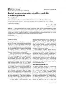
where u(k) is the control pressure, x(k) is the stem position, and y(k) is the flow through the valve which is the controlled variable. The input to the process, u(k), is constrained between [0; 1.2]. The nonlinear behavior of the control valve described by equation (26) is shown in Figure 1.

Figure 1. Static characteristic of a control valve. The space search adopted in PSO setup is: 0.01 ≤ φ (1) ≤ 0.50 , 0.10 ≤ ρ ≤ 5.00 , −1.00 ≤ η ≤ 1.00 , 0.01 ≤ λ ≤ 1.00 , and 1.00 ≤ µ ≤ 5.00 .

9 For the MFLAC design, the optimization procedure by PSO obtains

φ (1) = 0.366618 , ρ = 0.499131 , η = 3.662461 , λ = 1.375923 , µ = 0.391867 and fitness f = 0.8273 (best results in 30 runs). Simulation results for servo and regulatory responses of MFLAC are shown in Figures 2 and 3, respectively. Regulatory behavior analysis of the MFLAC was based on parametric changes in the plant output when: (i) sample 60: y(k) = y(k) + 0.2; (ii) sample 160: y(k) = y(k) - 0.2; (iii) sample 260: y(k) = y(k) – 0.4; (iv) sample 360: y(k) = y(k) + 0.4; and (v) sample 460: y(k) = y(k) + 0.4. Numerical results presented in Figures 2 and 3 show that the MFLAC using PSO approach have precise control performance. In Table 1, a summary of simulation results and performance of the MFLAC design based on PSO is presented. Table 1. Indices for the best MFLAC design using PSO. MFLAC mean of u variance of u mean of error variance of error

servo behavior 0.5474 0.1227 0.0160 0.0015

regulatory behavior 0.5535 0.1260 0.0123 0.0025

Figure 2. Input and output signals for the MFLAC (servo behavior).

Figure 3. Input and output signals for the MFLAC (regulatory behavior).

10


Conclusion and future research

Numerical results for controlling a control valve have shown the efficiency of the proposed MFLAC that guaranteed the convergence of the tracking error for servo and regulatory responses. However, it still has a distance to industrial applications and more practical issues must be done. A further investigation can be directed to analyze the PSO for model-free adaptive control methods [16] in essential control issues such as control performance, robustness and stability. References [1] F. Karray, W. Gueaieb, and S. Al-Sharhan, “The hierarchical expert tuning of pid controllers using tools of soft computing,” IEEE Transactions on Systems, Man, and Cybernetics  Part B: Cybernetics, vol. 32, no. 1, pp. 77-90, 2002. [2] K. J. Åström and T. Hägglund, PID controllers: theory, design, and tuning. Instrument Society of America, ISA, 1995. [3] B. H. Bisowarno, Y. -C. Tian, and M. O. Tade, “Model gain scheduling control of an ethyl tertbutyl ether reactive distillation column,” Ind. Eng. Chem. Res., vol. 42, pp. 3584-3391, 2003. [4] Z. Hou and W. Huang, “The model-free learning adaptive control of a class of siso nonlinear systems,” Proceedings of the American Control Conference, Albuquerque, NM, pp. 343-344, 1997. [5] Z. Hou, C. Han, and W. Huang, “The model-free learning adaptive control of a class of MISO nonlinear discrete-time systems,” IFAC Low Cost Automation, Shenyang, P. R. China, pp. 227232, 1998. [6] J. F. Kennedy, R. C. Eberhart and R. C. Shi, Swarm intelligence, Morgan Kaufmann Pub, San Francisco, USA, 2001. [7] Y. Shi and R. C. Eberhart, “Parameter selection in PSO optimization,” Proceedings of the 7th Annual Conf. Evolutionary Programming, San Diego, CA, USA, pp. 25-27, 1998. [8] K. Yasuda, A. Ide, and N. Iwasaki, “Adaptive particle swarm optimization,” Proceedings of IEEE Int. Conf. on Systems, Man and Cybernetics, Washington, DC, USA, vol. 2, pp. 1554-1559, 2003. [9] D. Devicharan and C. K. Mohan, “Particle swarm optimization with adaptive linkage learning,” Proceedings of the IEEE Congress on Evol. Computation, Portland, OR, USA, 530-535, 2004. [10] R. Mendes and J. F. Kennedy, “The fully informed particle swarm: simper, maybe better,” IEEE Transactions on Evolutionary Computation, vol. 8, no. 3, pp. 204-210, 2004. [11] R. A. Krohling, F. Hoffmann, and L. S. Coelho, “Co-evolutionary particle swarm optimization for min-max problems using Gaussian distribution,” Proceedings of Congress on Evolutionary Computation, Portland, USA, 959-964, 2004. [12] J. F. Kennedy and R. C. Eberhart, “Particle swarm optimization,” Proceedings of IEEE International Conference on Neural Networks, Perth, Australia, pp. 1942-1948, 1995. [13] R. C. Eberhart and J. F. Kennedy, “A new optimizer using particle swarm theory,” Proceedings of International Symposium on Micro Machine and Human Science, Japan, pp. 39-43, 1995. [14] A. Ratnaweera, S. K. Halgamuge, and H. C. Watson, “Self-organizing hierarchical particle swarm optimizer with time-varying acceleration coefficients,” IEEE Transactions on Evolutionary Computation, vol. 8, no. 3, pp. 240-255, 2004. [15] T. Wigren, “Recursive prediction error identification using the nonlinear Wiener model,” Automatica, vol. 29, no. 4, pp. 1011-1025, 1993. [16] J. C. Spall and J. A. Cristion, “Model-free control of nonlinear systems with discrete time measurements,” IEEE Transactions on Automatic Control, vol. 43, pp. 1198-1210, 1998.