Applying Probabilistic Mixture Models to Semantic Place Classification

Applying Probabilistic Mixture Models to Semantic Place Classification in Mobile Robotics Cristiano Premebida, Diego R. Faria, Francisco A. Souza, Urbano Nunes Abstract— In this paper a study is made of the problem of classifying scenarios, in terms of semantic categories, based on data gathered from sensors mounted on-board mobile robots operating indoors. Once the data are transformed to feature space, supervised classification is performed by a probabilistic approach called Dynamic Bayesian Mixture Models (DBMM). This approach combines class-conditional probabilities from supervised learning models and incorporates past inferences. In this work, several experiments on multi-class semantic place classification are reported based on publicly available datasets. Such experiments were conducted in a such way that generalization aspects are emphasized, which is particularly important in real-world applications. Benchmark results show the effectiveness and competitive performance of the DBMM method, in terms of classification rates, using features extracted from 2D range data and from a RGB-D (Kinect) sensor.

I. I NTRODUCTION In order to perceive and understand the surrounding environment, a mobile robot primary depends on data acquired from on-board sensors, being cameras (mono, stereo), laserscanners (2D, 3D) and RGB-D the most common employed sensors. Among the various tasks that can be performed by a robot, the ability to build a consistent map of the environment and to estimate the robot’s pose is of particular interest [1], [2]. To build a map, a mobile robot moves along a trajectory while collecting data from sensors and uses such sensory information to perceive the environment and construct the map concurrently. Maps can be represented, for example, in terms of metric coordinates or semantic descriptions; the latter is particularly useful in graph-based SLAM. The ability to understand and associate semantic terms such as “corridor” or “office” with places gives a much more intuitive idea of the location of the mobile robot in complement to metric coordinates. The process of applying a semantic term to some place of the map is also known as semantic mapping [3], [4], [5], [6]. Semantic classification of places has been an active research topic in robotics, and also in the machine vision community, wherein the majority of methods use features extracted from images (depth [6], monocular [7], [8], omnidirectional [9], [10]), from laserscanners [4], [11], [12], or a combination of vision and laser-range features as in [5]. Higher-level features can be explored, as in [2] where spatial semantics and objects are used in a Bayesian framework. In terms of pattern recognition techniques, discriminative or The authors are with the Department of Electrical and Computer Engineering, Institute of Systems and Robotics, University of Coimbra, Portugal. {cpremebida,diego,urbano}@isr.uc.pt. The third author is also with the Dept. of Electrical Engineering, Univ. Federal of Ceara, Brazil. {alexandre}@dee.ufc.br.

generative solutions have both been used in this research topic namely, Boosting techniques [13], Support Vector Machine (SVM) [9], [11], Naive Bayes classification [7], transfer learning [8], logistic regression [12], Bayesian [2], dynamic time warping and bag-of-words [10], conditional random fields (CRF) [5], and combination of techniques e.g., CRF+SVM as in [4]. In this work, place categorization using 2D laserscanner is particularly emphasized, motivated by three reasons: (1) this is an active sensor modality which is very robust against illumination changes (as shown in the results reported in Section IV); (2) laserscanners are extensively used in robotic applications in academia and industry (guaranteeing safe navigation); (3) most of the range-based features can be directly extrapolated to 3D lasers. Regarding the classification algorithm, a probabilistic approach that follows the principles of a dynamic Bayesian network [14] is used. This approach, with a mixture of probabilistic models in its structure, is named Dynamic Bayesian Mixture Models (DBMM) [15]. This method is tested and compared with a state-of-the-art classifier (a SVM) in terms of classification performance on laserscanner based datasets; nevertheless, experiments using RGB-D are also reported. Concerning experimental evaluation, three benchmark databases (detailed in [16], [17], [18] respectively) with data collected from mobile robots navigating in indoor scenarios were used for experiments. The contributions of this paper to the problem of place classification in mobile robotics applications are: (i) a general probabilistic approach that combines different classconditional probabilities, allowing flexibility and improvement in classification performance; (ii) a-posteriori outputs are smoothed by means of past probabilities incorporated in the DBMM model with the purpose of mitigating eventual abrupt changes in the likelihood response; (iii) this work reports thorough experiments highlighting generalization aspects, which is particularly important in real-world applications. The remainder of this paper is organized as follows. A brief review of mixture models and a description of the proposed DBMM method are presented in Section II. Datasets are described in Section III. Experimental results are reported and discussed in Section IV, emphasizing experiments in semantic place categorization using 2D-laserscanners. Finally, Section V concludes this paper. II. DYNAMIC BAYESIAN M IXTURE M ODELS : DBMM The DBMM is formulated in terms of a joint probability that takes into account the observed feature vector X, the set

of classes C, and past inferences D. The concept of mixture models is used and integrated into our dynamic Bayesian process where conditional probabilities from different base classifiers are weighted into a single probabilistic output. The next subsections present the general structure of the DBMM and how the weights are computed in order to assign confidence to the base classifiers.

3E

P(C1)t͙W;s)t Priors

P(X|C)t

6

P(C|X,D)t-1

w2

w1 BC1

wn

͙

BC2

P(C|X,D)t-T Xt1

A. Mixture Models A mixture model is here understood as a weighted combination of component probabilities, assumed independently distributed, that were modeled according to base classifiers (BCs). Considering the set of classes C and the classconditional probabilistic outputs from n base classifiers Pi (X|C)i=1,...,n , the general mixture model outputs a weighted probability P(X|C) as follows:

P(C|X,DT)t

Frames:

Ft-T

͙

Ft-2

Ft-1

Xt2

Weights Base Classifiers

BCn

͙ Xtn

Ft

Feature vectors

͙

Timeline

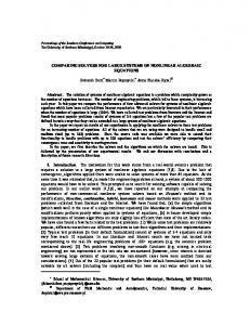
Fig. 1. Illustrative representation of the DBMM approach, where the posterior P(C|X, DT )t depends on the priors P(C), the combined likelihood P(X|C), the time-conditional probabilities (past inferences), and the normalization β .

n

P(X|C) = ∑ wi Pi (X|C),

(1)

i=1

where n is the number of base classifiers and wi is the weight associated to a given probabilistic output Pi (X|C) obtained by a supervised classifier. The weights, that sum to one ∑ni=1 wi = 1, were estimated by an Entropy-based measure as confidence level, as explained in Section II-C. B. The DBMM structure The DBMM structure is composed of a mixture model that outputs P(X|C)t (1), the a-priori class probabilities P(C)t , and past inferences, as illustrated in Fig. 1. The past inferences enters into the DBMM in the form of a time-based element DT that specifies a set of prior states given a time slice T i.e., DT = {Dt−1 , Dt−2 , · · · , Dt−T }. In the DBMM the general joint probability is expressed as: P(DT , X,C) =

t−T

∏

P(Dk |

k=t−1

t−T ^

D j , X,C) × P(X|C) × P(C), (2)

j=k−1

where the chain-decomposition of DT will be considered to be conditionally independent given (X,C) e.g., P(Dt−1 |Dt−2 , X,C) = P(Dt−1 |Dt−2 ). The joint probability (2) can be rewritten as P(C, X, DT ) and, after decomposition and arrangement, the posterior P(C|X, DT ) can be expressed as P(C|X, DT ) = β P(DT , X,C), where β is a normalization term to ensure a valid probability. For a specific time instant t, the DBMM model assumes the form: P(C|X, DT )t = β

t−T

∏

k=t−1

n

P(Dk |Dk−1 ) × ∑ wi Pi (X t |C) × P(C)t (3) i=1

where, for instance, the first element inside the multiplication operator takes the value of the previous posterior i.e., P(Dt−1 |Dt−2 ) ← P(C|X, DT )t−1 , and so on. C. Assigning Weights using Entropy In the DBMM framework we use Entropy H, from information theory, as a confidence level to estimate the weights w that will be used to compose the mixture of classifiers.

Considering a training set comprising the likelihoods delivered by the set of base classifiers, Entropy is computed as follows: H(Pi (A)) = − ∑ Pi (A) log(Pi (A)), (4) i

where, in our case, Pi (A) = Pi (C|X) represents the conditional probability given the model of a ith classifier and the set of features X = {x1 , x2 , ..., xm }. From the learning stage (i.e., using a training set), the set of likelihoods assumes the form of a probability density function (pdf ). Knowing H, the weight wi for each ith classifier is estimated as the distribution inversely proportional to Entropy as follows:   1 − ∑nHi Hi  , i = {1, ..., n},  i=1 (5) wi = H ∑ni 1 − ∑n i Hi i=1

where Hi is the value of Entropy resultant from (4). The denominator in (5) guarantees that ∑i wi = 1. This weighting strategy will smooth the base classifier’s response by continuously multiplying its classification belief by the correspondent weight. III. B ENCHMARK DATASETS In this Section, the semantic place labeling datasets used in the experiments are briefly described (these datasets are publicly available on the Web). The first dataset was collected from three indoor environments of buildings 52, 79 and 101 at the University of Freiburg (named FR52, FR79 and FR101 respectively), and are composed by the classes “corridors”, “rooms”, “doorways”, while FR101 has an additional class “hall”. The second dataset considered here is one of the three sub-datasets that composes the COLD database [17], namely we used the Saarb-dataset because of two reasons: it has a greater number of classes than others COLD’s sub-sets, and it provides laserscanner data with adequate resolution while Ljubl-dataset has laser data but with low resolution. The RGBD-based dataset, detailed in [18], is composed of a set of vision-based features extracted from a Kinect sensor and is characterized by five classes. Table I shows a summary

TABLE I

S UMMARY OF FR S , COLD-S AARB AND RGB-D DATASETS .

TABLE II WITH

Dataset FR52 FR79 FR101 COLD Saarb

Classes corridor, rooms doors corridor, rooms doors corridor, rooms doors, hall 9 classes*

#Fea. 50 50 50 50*

room, corr., RGBD 397 kit., labs, office (*) See Section III-B for details.

N# of examples Train: (7396, 43957, 1112) Test: (6093, 32214, 743) Train: (16687, 43624, 1449) Test: (15516, 50180, 701) Train: (858, 9005, 262, 18095) Test: (931, 6795, 243, 26688) N# of examples depends on the experiments* (252, 279, 191, 357, 149) N# depends on a random 10-fold

of these datasets, where the numbers of examples of each class is given in parentheses. A. Datasets (FR52, FR79 and FR101) and features In the FRs datasets, and also in the COLD-Saarbr¨ucken database (Section III-B), the mobile robot is equipped with a 2D laserscanner covering a field of view around the robot. A given sensor measurement, z = {b0 , . . . , bm }, contains a set of laser-beams bi , where 0 ≤ i ≤ m. Each beam bi consists of a pair bi = (αi , di ), where αi is the angle of the beam relative to the robot and di is the length of the beam. Mozos et al. [13] have proposed the use of a set of geometrical features extracted from range scans (the so called B and P-features). These features are invariant to robot rotation, making them dependent on the robot position and not on its orientation. Thus, for each incoming laserscan, the B-features are calculated using the raw beams in z, while the P-features are calculated from a polygonal approximation P(z) of the area covered by z. The vertexes of the closed polygon P(z) correspond to the Cartesian coordinates of the end-points of the laser-beams in z: P(z) = {(di cos αi , di sin αi ) | i = 0, . . . , m + 1}. In this work, we actually employed a subset of the B & P-features. The components of our feature vector are summarized in Table II showing the correspondence with the B & P-features proposed in [13]. We noticed that the feature B.3 has constant value, and hence it was not considered, while feature P.6 - which corresponds to coefficients 2 to 100 of Fourier transform - tends to induce overfitting problems and thus it was discarded. B. COLD Saarbr¨ucken dataset The COLD-Saarb sequences were acquired under different weather and illumination conditions (designated by Cloudy, Night, Sunny), and across a time span of two/three days [9]. The Saarb-set has 9 classes: “Corridor”, “Terminal room”, “Robotic lab”, “1-person office”, “2-persons office”, “Conference room”, “Printer area”, “Kitchen”, and “Bath room”. Two paths were followed by the robot during data acquisition, the Standard and the Extended paths; moreover, sequences of the dataset were annotated as portions A and B: the main difference is that those parts annotated as “A” do not have sequences under “Sunny” condition (see [9] for

F EATURE COMPONENTS AND THEIR CORRESPONDENCE B & P- FEATURES AS ORIGINALLY PRESENTED IN [13]

Features x1,2,3,4 x5 , . . . , x24 x25,26,27,28 x29 , . . . , x38 x39 x40,41,42 x43,44 x45,46,47 x48,49 x50

Description correspond to features B.1, B.2, B.5, B.6; correspond to feature B.7 with thresholds 0.5m to 10.0m (0.5m steps); correspond to features B.11, B.12, B.13, B.14; correspond to feature B.15 with thresholds 0.1m to 1.0m (0.1m steps); corresponds to feature B.16; correspond to features P.1, P.2, P.3; correspond to features P.4, P.5; correspond to features P.7, P.8, P.9; correspond to features P.16, P.17; corresponds to feature P.15;

more details). This dataset provides, among mono and Omniimage frames, raw laser scans with FOV=180◦ and 0.5◦ of resolution i.e., each laser scan has 361 points. In order to allow a consistent analysis, we opted to extract the same B & P features (see Table II) to compose a classification set with 50 features. C. Kyushu University Kinect place recognition dataset This dataset contains RGB-D images acquired by a Kinect sensor mounted onboard a mobile platform. Five classes are considered: “corridor”, “kitchen”, “labs”, “office” and “room”. This dataset was recorded from a mobile robot driving through different buildings of the Kyushu University [18]. To perform semantic place categorization, histograms of local binary pattern (LBP) were extracted from grayscale and depth images in order to compose a feature vector as described in [18]. Moreover, the dimensionality of each histogram was further reduced by selecting a subset of their LPB’s using a uniformity measurement introduced in [19]. A threshold (θ ) is used to control such uniformity measurement, where lower values of θ produce histograms with reduced dimensionality. IV. E XPERIMENTS AND PERFORMANCE EVALUATION In this Section, the DBMM method is evaluated in terms of classification performance on the semantic place labeling datasets described in Section III. In the FRs datasets, classification performance is assessed by applying Fmeasure = Pr·Re , calculated on the testing part of the datasets, where 2 Pr+Re Pr and Re denote precision and recall respectively. Unlike in [13], [16] where accuracy is used as performance measure, here we primary adopted Fmeasure 1 because all datasets have unbalanced classes. On the other hand, and to follow the same methodology described in [18], average accuracy is used to assess performance in the RGB-D dataset. In the COLD-Saarb bar charts are used to report classification rates, enabling a direct comparison with the results in [9]. The experiments are firstly conducted using a SVM (using libSVM2 ) and the DBMM within the FR’s scenarios (intra1 In this paper the values of F measure are presented 2 http://www.csie.ntu.edu.tw/˜cjlin/libsvm/

in percentage.

TABLE III

Perf. F¯measure Re(corr.) Re(room) Re(door) Re(hall)

(a) FR52 train.

E VALUATION OF A SVM ( TESTING SET )

fea.B (#n = 39) fea.P (#n = 11) B & P (#n = 50) FR52 FR79 FR101 FR52 FR79 FR101 FR52 FR79 FR101 71.20 94.86 99.86 13.06 -

68.17 99.12 94.46 23.82 -

56.00 35.77 93.35 7.00 93.73

65.29 69.07 96.44 98.56 99.78 100.0 0.0 4.99 -

SVM

AND

DBMM

PERFORMANCE ON THE

SVM Performance FR52 FR79 FR101

(e) FR101 train.

72.08 97.67 99.90 12.11 -

68.50 99.35 94.61 25.25 -

59.37 53.28 92.38 11.52 93.81

(b) FR52 test. TABLE IV

(c) FR79 train.

61.47 69.92 92.88 14.40 89.82

(d) FR79 test.

(f) FR101 test.

Fig. 2. Maps exhibiting the DBMM classification results for the FR52, FR79 and FR101 buildings; — Corridors (in red); — Rooms (in blue); — Doorways (in yellow); — Hall (in cyan). See text for details.

buildings), and their results are analyzed and discussed in the Section IV-A. Seeking to verify the performance on “unseen” environments, in Section IV-B we report results in terms of generalization capabilities (cross-building). Secondly, and following the methodology in [9], Section IV-C brings two series of experiments on the Saarb-dataset: (1) where differences in illumination conditions and categorical aspects are considered, and (2) different paths (Standard and Extended) are interchanged between training and testing sets, which allows analysis in terms of generalization capacity. The experiments are concluded with Section IV-D, where the results using the RGBD dataset are presented. A. Intra-building semantic classification In a first experiment, a SVM was trained having as input normalized values of the features from Table II, and the results regarding the FR52, FR79 and FR101 testing sets are summarized in Table III. The results are reported by feature type, i.e., features of type B (left), P (center) and in the last column all features are used; F¯measure denotes the average value of the Fmeasure for all classes. From the results shown in Table III, one can conclude that the subset of P-type features has a good discriminative capacity (see values in bold for FR79 and 101), keeping low complexity: only 11 features. On the other hand, in the FR52 scenario the combination of B&P features achieved better results. Concerning the class “Doors”, the results are significantly lower in comparison

F¯measure Re(corr.) Re(room) Re(door) Re(hall)

72.08 69.07 97.67 98.56 99.90 100.0 12.11 4.99 -

61.47 69.92 92.88 14.40 93.81

FR

DATASETS

DBMM FR52 FR79 FR101 70.92 96.04 99.96 10.63 -

75.75 98.85 100.0 17.26 -

63.75 71.64 94.61 15.23 91.17

with other classes; the most likely explanation is because “Doors” is much less frequent than others classes (see Table I) and thus the classifier tends to favor the majority classes. The DBMM is used in a second experiment, where the mixture model inside the DBMM contains two base classifiers (n = 2 in Fig. 1) as class-conditional probabilities i.e., BC1 is a SVM using the 39 B-features (X1 = f ea.B) and BC2 is another SVM using the 11 P-features (X2 = f ea.P). This strategy keeps the complexity of the DBMM consistent with the SVM used in the first experiment. Classification results achieved by the proposed DBMM are shown in Table IV, as well as the best results (in terms of F¯measure ) obtained by the SVM are also presented to make comparison easier. The results indicate the effectiveness of the DBMM, obtaining best generalization in two scenarios (FR79 and 101) while keeping the complexity i.e., the amount of features, equivalent to the benchmarked SVM. Figure 2 exhibits the maps of the buildings, where each place is indicated by its respective color. The training sets are shown in the left part of Fig. 2, while the semantic outputs using the DBMM algorithm are illustrated in the right part. Notice that the classifier had difficulties in classifying “Doorways” (in yellow): the lower number of examples and the appearance on narrow FOV are explanations for these results. Moreover, in the highlighted region at the testing part of FR101 the performance suffered a degradation, meaning that the number of false positives at that region increased (i.e., Pr decreased). B. Cross-building semantic classification Looking to verify the performance in unseen environment i.e., the generalization capability of the methods in ‘new’ scenarios, in this Section the classification methods are trained in one dataset and tested in other set (for that purpose, buildings 52 and 79 were considered). The models were trained using the dataset collect in the FR52 building and then tested on the dataset acquired at FR79 building, and vice-versa. Results are summarized in Table V. With respect

E VALUATION OF SVM AND DBMM ON CROSS - BUILDING

Training in STD Cloudy

100

Cloudy

98.11

66.53

70.50

95.81

PO

90.68

CR

96.86

43.72

41.77

TL

PA

TL

PA

PO

CR

TL

PA

PO

CR

TL

PA

TL

PA

PO

CR

TL

PA

10

PO

Sunny

0

91.42

92.43

96.07

86.06

89.18

89.82

92.09

92.56

93.49

94.83

91.18

89.80

92.76

Testing in EXT

80

Hit rate [%]

87.22

40

CR

Night

90

70

Sunny

20

Training 100

69.69

50

30

Cloudy

Night

86.97

96.47 84.89

97.45 71.31

60

95.58

70

PO

67.64 97.52 88.70 44.64

92.16

65.47 92.84 86.30 45.82

CR

75.61 93.73 99.98 31.77

71.70

74.86 94.17 99.92 27.58

80

97.71

DBMM

82.31

SVM

91.43

DBMM

97.34

SVM

Training in EXT Sunny

90

84.70

Trained in FR79 tested in FR52

Hit rate [%]

Perf. F¯measure Re(corr.) Re(room) Re(door)

Trained in FR52 tested in FR79

Night

74.58

TABLE V

Testing in STD

Fig. 4. Hit rate performance, per class, considering non-correlated scenarios: trained on the Standard-set and tested on the Extended-set (bar charts in the left), and vice-versa (right part). Four categories were tested: corridor (CR), person-office (PO), printer-area (PA), and toilet-room (TL).

60 50 40 30

Std B

Std B

Std B

Std B

Std B

Std B

Std B

Std B

Std A

Std B

Su

Std A

Std A

N

Su

C

C

N

N

C

10

Std A

20

0

ht

ig

N y

ud

y

y

nn

lo

C

Su

nn

y

y

ud

lo

ht

ig

ud

lo

ht

ig

C

N

y

nn

ht

y

ud

ig

lo

ht

ig y

ud

lo

Testing

(a) Standard (Std) sequence Training Cloudy

100

Night

Sunny

93.79

89.50

96.51

88.25

86.07

76.66

76.43

86.85

77.17

60

74.35

Hit rate [%]

70

84.94

94.39

80

90.88

90

50 40 30

Ext B

Ext B

Ext B

Ext B

Ext B

Ext B

Ext A

Ext B

Ext A

Ext B

N

Ext B

C

Ext A

Su

Su

Su

N

C

C

N

N

C

C

10

Ext A

20

0

ht

ig y

y

ud

nn

lo

y

y

y

ud

nn

lo

ht

ud

ig

ht

lo

ig

N

y

y

nn

ht

y

ud

ig

lo

ht

ud

ig

lo

Testing

(b) Extended (Ext) sequence Fig. 3. Results are presented per illumination condition in terms of overall hit rate calculated over all classes. Each bar shows the sequence (Std,Ext) and the portion (A,B) used in the testing data e.g., StdA denotes Standard sequence of the portion A.

to the first case, the DBMM method obtained the best value of F¯measure due to a better balance between precision and recall, in particular for class “Doors”. In the second case (right part of Table V), the best F¯measure result was again obtained by the DBMM but, this time, the class “Corridor” contributed more. Overall, results exhibit a balanced performance between the cases. C. Experiments on COLD-Saarb This Section starts with experiments on the Standard and Extended parts, and the portions “A” and “B”, in accordance with the experiments carried out in [9]. The main goal of these experiments is to evaluate place recognition under varying illumination and categories (classes) settings. Essentially, the training and testing sets differ as function of the weather and illumination conditions (Cloudy, Night, Sunny). Here, as in the experiments using the FRs dataset, the mixture

model used in the DBMM structure was built with two SVM classifiers, learned with B and P features respectively. The results shown in Fig. 3 were grouped according to the sequence type (Standard or Extended), the portions of the scenario (‘A’ or ‘B’), and the weather/illumination conditions used for training and testing. As in [9], bottom axes indicate the conditions used for testing, while top axes refer the conditions on training. These results allow us to conclude that DBMM achieved an average classification performance of 91.67% and 85.82%, which surpass SVM (narrow bars depicted within the gray-bars), and also the solution in [9]. Furthermore, our solution using laser-based features demonstrates to be robust under variations of illumination. Figure 4 shows recall, or hit rate, for the four classes that are all available in the two paths followed by the robot (sequences Std and Ext). This experiment explores the situation where the classification method is trained and tested in sequences whose conditions are substantially different and therefore, it allows us to study cross-dataset generalization. In general, the performance on classes ‘CR’ and ‘PO’ are very good, while the accuracy on classes ‘PA’ and ‘TL’ degrades in some conditions; an explanation is that the training and testing set are very unbalanced. This is particularly evident, for instance, in the “STD-Sunny” subset where the training set has (821, 364, 325, 828) elements while the testing set “EXT” (which includes all sub-sets) has (9726, 2346, 1841, 3292) elements. In general, DBMM achieved better results than SVM. Further discussions are provided in Section IV-E. D. RGB-D place recognition In the experiments on laserscanner-based datasets, only SVMs were used as base classifier, however in the experiments on the RGB-D dataset an Artificial Neural Network (ANN) classifier is also employed. As consequence, the DBMM was trained with two heterogeneous base classifiers, one SVM (BC1 ) and one ANN (BC2 ), having both classifiers the same number of features #Fea=397 and the same feature vector i.e., X1 = X2 . To evaluate the classification performance in this dataset, this paper follows the same

TABLE VI

E VALUATION ON THE RGB-D DATASET.

ANN SVM DBMM θ = 2 89% ± 0.086 89% ± 0.085 91% ± 0.079 θ = 4 92% ± 0.074 91% ± 0.076 94% ± 0.061 θ = 8 92% ± 0.090 91% ± 0.078 93% ± 0.075

procedure described in [18]: each testing set was created by randomly selecting one place from each category, while the remaining places are used for training purpose. This methodology assures that testing sets contain examples from places that do not appear in the training part. Experiments using three subsets of LBPs features were performed based on values of thresholds θ applied as function of an uniformity measurement [18]. For θ = {2, 4, 8}, the aforementioned procedure is repeated 10 times and the average accuracy is reported, as well as the standard deviation. Table VI shows the results using the 10-fold randomvalidation strategy and averaging the performance across the folds for the models trained and tested separately. According the results from Table VI, the proposed DBMM ranks as the best approach. E. Discussion Experiments on the FR datasets are very detailed, and the goals were to study the potentialities of solutions using 2D-laser based features and to conduct systematic analysis of the DBMM’s performance in comparison with SVM. The latter was chosen because SVM is one of the most common and effective method used in this field. Regarding the first experiments on the COLD-Saarb dataset, which contains more classes than FRs and RGB-D datasets, the DBMM achieved a higher classification rate relative to the image-based solution in [9]. The second experimental part, summarized in Fig. 4, constitutes a new experiment conducted on this dataset. Finally, the experiments on the RGBD dataset had the purpose of exploring the DBMM with a more complex feature-set and using heterogeneous base classifiers in its mixture model. Classification performance was compared with a SVM and an ANN (table VI), and the implemented DBMM obtained higher accuracy and lower deviations. V. C ONCLUSION In this study we carried out many experiments on semantic place recognition, in the context of mobile robotics applications, to assess the state of the art in this topic. Particular focus was devoted to publicly available datasets using 2D-laserscanner. In addition to the experimental part and analysis, this paper contributes with a probabilistic framework (called DBMM), that uses mixture models and temporal-inference in its structure. From the several experiments carried out on semantic place recognition, the DBMM demonstrated to be a very promising approach. In summary, the results reported in this work show that the DBMM is a very competitive method, reaching better classification

results than benchmarked solutions, with interesting characteristics: (i) DBMM supports general probabilistic classconditional models; (ii) dynamic information in the form of temporal/prior inferences can be incorporated; (iii) diversity on the base-classifiers are suitable to be controlled in a direct manner. DBMM allows fast implementation and direct probabilistic interpretation. ACKNOWLEDGMENT This work has been supported by the FCT project “AMSHMI2012-RECI/EEIAUT/0181/2012” and project “ProjB: Diagnosis and Assisted Mobility - Centro-07-ST24-FEDER002028” with FEDER funding, programs QREN and COMPETE. We also thank the reviewers for their valuable comments and suggestions. R EFERENCES [1] M. Milford, “Vision-based place recognition: how low can you go?” The International Journal of Robotics Research, vol. 32, no. 7, pp. 766–789, 2013. [2] S. Vasudevan and R. Siegwart, “Bayesian space conceptualization and place classification for semantic maps in mobile robotics,” Robotics and Autonomous Systems, vol. 56, no. 6, pp. 522–537, jun 2008. [3] A. Pronobis and P. Jensfelt, “Large-scale semantic mapping and reasoning with heterogeneous modalities,” in ICRA, IEEE, 2012. [4] L. Shi, S. Kodagoda, and G. Dissanayake, “Application of semisupervised learning with voronoi graph for place classification,” in IROS, IEEE/RSJ, 2012. [5] L. Shi, S. Kodagoda, and M. Piccardi, “Towards simultaneous place classification and object detection based on conditional random field with multiple cues,” in IROS, IEEE/RSJ, 2013. [6] H. Jung, O. Martinez Mozos, Y. Iwashita, and R. Kurazume, “Indoor place categorization using co-occurrences of LBPs in gray and depth images from RGB-D sensors,” in Emerging Security Technologies (EST), 2014 Fifth International Conference on, Sept 2014. [7] J. Wu, H. Christensen, and J. Rehg, “Visual place categorization: Problem, dataset, and algorithm,” in IROS, IEEE/RSJ, 2009. [8] G. Costante, T. Ciarfuglia, P. Valigi, and E. Ricci, “A transfer learning approach for multi-cue semantic place recognition,” in IROS, IEEE/RSJ, 2013. [9] M. Ullah, A. Pronobis, B. Caputo, J. Luo, R. Jensfelt, and H. Christensen, “Towards robust place recognition for robot localization,” in ICRA, IEEE, 2008. [10] L. Yuan, K. C. Chan, and C. George Lee, “Robust semantic place recognition with vocabulary tree and landmark detection,” in IROS’s Workshop, IEEE, 2011. [11] P. Sousa, R. Araujo, and U. Nunes, “Real-time labeling of places using support vector machines,” in Industrial Electronics, 2007. ISIE 2007. IEEE International Symposium on, June 2007. [12] L. Shi, S. Kodagoda, and G. Dissanayake, “Laser range data based semantic labeling of place,” in IROS, IEEE/RSJ, 2010. [13] O. M. Mozos, Semantic Place Labeling with Mobile Robots. Springer, Tracts in Advanced Robotics (STAR), 2010. [14] V. Mihajlovic and M. Petkovic, “Dynamic Bayesian Networks: A State of the Art,” Technical reports series, TR-CTIT-34, 2001. [15] D. Faria, C. Premebida, and U. Nunes, “A probabilistic approach for human everyday activities recognition using body motion from RGBD images,” in RO-MAN, IEEE, 2014. [16] O. M. Mozos, A. Rottmann, R. Triebel, P. Jensfelt, and W. Burgard, “Supervised semantic labeling of places using information extracted from sensor data,” Robotics and Autonomous Systems, vol. 55, pp. 391–402, 2007. [17] A. Pronobis, O. M. Mozos, B. Caputo, and P. Jensfelt, “Multi-modal semantic place classification,” The International Journal of Robotics Research (IJRR), vol. 29, no. 2-3, pp. 298–320, 2010. [18] O. M. Mozos, H. Mizutani, R. Kurazume, and T. Hasegawa, “Categorization of indoor places using the kinect sensor,” Sensors, vol. 12, no. 5, pp. 6695–6711, 2012. [19] T. Ojala, M. Pietikainen, and T. Maenpaa, “Multiresolution gray-scale and rotation invariant texture classification with local binary patterns,” IEEE TPAMI, vol. 24, no. 7, pp. 971–987, 2002.