Francine Berman. â. â. Computer Science and ... [ssmallen,casanova,berman]@cs.ucsd.edu. Abstractâ ...... Steve Young, and Mark Ellisman. Combining Work-.
Applying Scheduling and Tuning to On-line Parallel Tomography Shava Smallen ∗
∗
Henri Casanova
∗
Francine Berman
∗
Computer Science and Engineering Department University of California, San Diego USA [ssmallen,casanova,berman]@cs.ucsd.edu
Abstract—
availabilities. We demonstrate that application scheduling/tuning can be framed as multiple constrained optimization problems and evaluate our methodology in simulation. Our results show that prediction of dynamic network performance is key to efficient scheduling and that tunability allows for production runs of on-line parallel tomography in Computational Grid environments.
Tomography is a popular technique to reconstruct the three-dimensional structure of an object from a series of two-dimensional projections. Tomography is resource-intensive and deployment of a parallel implementation onto Computational Grid platforms has been studied in previous work. In this work, we address on-line execution of the application where computation is performed as data is collected from an on-line instrument. The goal is to compute incremental 3-D reconstructions that provide quasi-real-time feedback to the user.
Keywords— Application Level Scheduling Application Tunability Heterogeneous Computing Computational Grid Parallel Tomography On-line Instruments Soft Real-time
We model on-line parallel tomography as a tunable application: trade-offs between resolution of the reconstruction and frequency of feedback can be used to accommodate various resource This research was supported by NSF grants ACI-9701333 and ACS-9619020. Equipment used in this research was supported in part by the UCSD Active Web Project, NSF Research Infrastructure Grant Number 9802219.
I. Introduction Tomography is a widely used technique to reconstruct the three-dimensional structure of an object from a series of two-dimensional projections [1]. Several reconstruction algorithms are inherently parallel [1, 2, 3]. With these algorithms, the three-dimensional volume or tomogram can be decomposed into slices such that each slice is computed independently.
Permission to make digital or hard copies of all or part of this work for personal or classroom use is granted without fee provided that copies are not made or distributed for profit or commercial advantage, and that copies bear this notice and the full citation on the first page. To copy otherwise, to republish, to post on servers or to redistribute to lists, requires prior specific permission and/or a fee. SC2001 November 2001, Denver (c) 2001 ACM 1-58113293-X/01/0011 $5.00
1
One can envision two scenarios for running parallel tomography: off-line and online. In off-line parallel tomography, the user runs tomography on a dataset that resides on secondary storage to obtain a single, highresolution tomogram as quickly as possible. Conversely, on-line parallel tomography operates on data as it is collected from an on-line instrument. The goal is to compute successive tomograms in quasi-real-time to provide feedback on the quality of the data acquisition. In previous work, we and our collaborators developed a parallel implementation of off-line tomography called GTOMO (Grid TOMOgraphy) [4]. This implementation is currently used in production at the National Center for Microscopy and Imaging Research (NCMIR). GTOMO is used to reconstruct the threedimensional structure of biological specimens at the cellular and sub-cellular level using twodimensional projections collected from a powerful electron microscope. In this paper, we address the on-line scenario. We target on-line parallel tomography to a Computational Grid (or Grid for short) [5, 6] composed of multi-user workstation clusters and supercomputers. Executing applications in this type of computing environment can be challenging because resource availability is dynamic. Our results show that quasi-real-time execution of on-line parallel tomography can be achieved using a strategy that combines application tunability [7] with application-level scheduling [8, 9]. This strategy has been incorporated into GTOMO and will be put in production at NCMIR. This paper is organized as follows. In Section II, we briefly review our work on off-line parallel tomography. We also describe on-line parallel tomography and motivate its implementation as a tunable application. Section III details our scheduling strategy for deploying on-line parallel tomography on a Grid. Sim-
ulation results are given in Section IV. Section V discusses related work and Section VI concludes the paper. II. From Off-line to On-line A. Tomography at NCMIR During a tomography experiment at NCMIR, a specimen is placed under an electron microscope and rotated about a single axis while p projections are acquired using a CCD camera. Typically 61 projections are acquired. The size of each projection depends on the resolution of the CCD camera, currently either 1k × 1k or 2k × 2k. We define a tomography experiment as E = (p, x, y, z) where p is the number of projections, x and y are the dimensions of the projections and z is the thickness of the object; x, y, and z are measured in pixels. Given the resolution of the CCD cameras, (61, 1024, 1024, 300) and (61, 2048, 2048, 600) are representative examples of NCMIR experiments. The tomography reconstruction techniques used by NCMIR (R-weighted backprojection [10], ART [11], SIRT [12]) are embarrassingly parallel. Figure 1 illustrates the parallelism of these techniques. The information required to produce the ith X-Z slice of the three-dimensional volume (or tomogram) is the ith scanline from all projections. Therefore, the three-dimensional volume can be decomposed into a series of X-Z slices where each slice is computed independently of the others. B. Off-line Parallel Tomography The target computing platform for NCMIR is a Grid composed of multi-user workstation clusters and supercomputers under different administrative domains. Leveraging this type of platform is challenging because resources are heterogeneous, dynamic, and under different administrative policies. Fortunately, several
2
driver
Z specimen
X
ptomo
Y
ptomo
ptomo
slice
sinogram
reader
ne
pro
n
tio
jec
scanli
writer slice
sinogram
disk
Fig. 1. Parallelism of tomography. The information required to reconstruct the i th X-Z slice is the i th scanline from all projections.
disk
Fig. 2. Off-line GTOMO architecture.
resource selection strategy that co-allocates the execution of parallel tomography over workstations and immediately available supercomputer nodes. The architecture of GTOMO is displayed in Figure 2. A multi-threaded reader process reads input data (called sinograms) from disk and sends that data to ptomo processes. Each ptomo process performs a part of the reconstruction and sends reconstructed slices to a writer process which writes the data back to disk. The figure also displays a driver process that coordinates all the different processes.
Grid infrastructure projects [13, 14, 15, 16, 17] are available to facilitate running an application across different administrative domains. Our implementation of off-line parallel tomography, GTOMO [4], uses services from the Globus toolkit [13] for remote job management, security, and interprocess communication. To address the heterogeneous, dynamic properties of a Grid [5], we use an application-level scheduling strategy. An AppLeS (application-level scheduler) [8] integrates with the target application to develop a schedule for deploying the application in a Grid environment. The scheduler makes predictions of the performance the application may experience on prospective resources at execution time. Using these predictions, a potentially performance-efficient schedule for the application is identified and deployed [18, 19, 20, 4]. For GTOMO, because our application is embarrassingly parallel, it is natural to use self-scheduling [21]. We opted for a greedy work queue algorithm where computation is assigned to processors as soon as they become available. The algorithm is also coupled with a
C. On-line Parallel Tomography Currently, NCMIR users run tomography on their data after they collect it from the electron microscope (off-line). Upon visualization of their data, they sometimes discover a misconfiguration of the microscope or might find a more interesting area of the specimen to study. In such cases, users must modify the microscope parameters and acquire a new dataset. This requires at least 45 additional minutes and increases beam damage to the specimen [22]. It would therefore be extremely
3
useful to provide feedback to the user by computing incremental tomograms during the acquisition process.
driver
ptomo
ptomo
ptomo
C.1 Extensions to GTOMO scanlines
To incrementally compute a tomogram, we update the ith slice of the tomogram with the ith scanline of each projection as it is acquired from the electron microscope. Achieving this in real-time requires a reconstruction technique that is fast and augmentable. An augmentable technique allows each successive computation to build upon the previous computation without repeating work. Fortunately, the R-weighted backprojection technique [10] fulfills both requirements.
preprocessor projection
slice
writer
tomogram
Fig. 3. On-line GTOMO architecture.
C.2 Tunability
The implementation of the R-weighted backprojection method as an augmentable technique mandates a modification of the GTOMO application. It requires that we send the ith scanline from each projection to the same ptomo process so that it may process the information into the same slice. Therefore, the work queue approach described in Section II-B is no longer viable and we replace it with a static work allocation strategy. We leave rescheduling for future work.
Because on-line parallel tomography is resource-intensive, we want to consider its execution on dynamic Grids with differing resource capabilities. Therefore, we have designed our implementation of on-line parallel tomography to be tunable. A tunable application is characterized by the availability of alternate configurations, where each configuration corresponds to a different execution path and resource usage [7]. In this work, tunability allows us to express trade-offs between tomogram resolution and the frequency of tomogram updates. We next illustrate its usage through an example. We define the acquisition period, a, as the time to acquire a projection from NCMIR’s electron microscope. NCMIR is currently targeting an acquisition period of 45 seconds; therefore, we use this value throughout our work. Consider a (61,2048,2048,600) experiment (see Section II-A) which yields a tomogram of about 9.4 GB. If we place our writer
The structure of on-line GTOMO is shown in Figure 3. The electron microscope sends a projection to the preprocessor every a seconds. The preprocessor divides the projection into sections, where each section contains multiple scanlines. The scanlines in each section will be processed in parallel by ptomo processes. All ptomos will periodically send their slices to the writer in order to update the tomogram. A visualization program will then display updated tomograms to the user. The driver coordinates interactions among all other processes.
4
on a machine with an observable bandwidth of 100 Mb/s, it will take 768 seconds to transfer the whole tomogram. To avoid overloading the network, we send only one tomogram at a time. So for this experiment, successive tomograms should be sent at least 768 seconds apart. Since a projection is processed every 45 seconds, we � = 18 projeccan send a tomogram every � 768 45 tions. We call each send a refresh and say that the number of processed projections per refresh is 18. The period of the refresh is 18×45 = 810 seconds, approximately 14 minutes. After surveying the requirements of NCMIR users, it appears that no user would tolerate a refresh periods which is over 10 minutes.
III. Scheduling We have defined the pair (f, r) that determines the configuration of the application. If enough resources were available, users would always choose (1, 1) which would result in the highest resolution tomogram being refreshed at the highest frequency possible. Given insufficient resources, in practice users need to choose an alternate configuration when the ideal configuration is infeasible. This choice depends on each user’s requirements; therefore our scheduler aims at assisting users in selecting an appropriate configuration. At run-time, the scheduler discovers which pairs are feasible and allows users to chose a pair that best fits their requirements for execution. The process of discovering feasible pairs is described in the following subsections.
Now, suppose we reduce the resolution of the projections by a factor of 2 in each dimension. For the time being we consider a simple averaging strategy [23]. The tomogram would then be 1.2 GB, 8 times smaller. Thus, it would take only 96 seconds to transfer each tomogram, yielding an acceptable refresh period of 135 seconds. Note that further reductions are possible but in order to yield a sufficiently detailed tomogram for NCMIR users, the projections should not be reduced beyond 256 × 256.
A. Constraints for On-line Tomography We evaluate on-line parallel tomography as a soft real-time application, one that is characterized by the execution of tasks which have soft deadlines [24]. That is, the usefulness of the task decreases as the tardiness of the task increases [24, 25]. Given the discussion in Section II-C, our soft deadlines are: (i) the computation time of one projection is less than the acquisition period, (ii) the transfer time of a tomogram is less than the refresh period. Our goal is to find a configuration of the application for which all deadlines are met. Consider a tomography experiment (p, x, y, z) and a pair (f, r). Our scheduler must allocate work to resources. For a set of compute resources M , we define a work allocation as a set W :
Two parameters, therefore, determine the quality of on-line parallel tomography: reduction factor and projections per refresh. The reduction factor (f ) is a scalar value that specifies a reduction of the size of a projection in each dimension. If we have a projection of size x × y, after reduction, we will have a projection of size fx × fy . Increasing the reduction factor decreases the number of slices and the amount of computation and communication per slice. The projections per refresh (r) parameter refers to the number of new projections processed into each successive tomogram refresh. An increase in r reduces the frequency of refreshes sent to the user and thus reduces the amount of communication.
W = {wm : m ∈ M }
(1)
where wm is the number of tomogram slices allocated to processor m.
5
where cpum is the fraction of CPU available on processor m. In practice we obtain a prediction for the value of cpum from the Network Weather Service (NWS) [26]. Likewise, for a space-shared supercomputer,
We have the two following constraints:
∀m ∈ M wm ≥ 0 � y wm = f m∈M
(2) (3)
Tcomp (m) =
y f
since there are a total of tomogram slices to compute. In the following two sections we derive constraints for the computation deadline and the communication deadline.
The soft deadline for computation can be written as: Tcomp (m) ≤ a,
(4)
where Tcomp (m) is the time to compute wm slices on processor m and a is the acquisition period. A simple analysis of the augmentable Rweighted backprojection algorithm used for the tomographic reconstruction shows that Tcomp (m) ≈ tppm ×
x z × × wm , f f
C. Communication deadline The soft deadline for data transfers can be written as: ∀m ∈ M
Tcomm (m) ≈
tppm x z × × × wm , cpum f f
(9)
wm × ( fx × Bm
z f
× sz)
,
(10)
where sz is the number of bits used to represent a pixel and Bm is the bandwidth between processor m and the writer. We can obtain predictions for Bm from the NWS [26]. Note this model assumes a fully connected network where each processor has a dedicated link to the writer. However resources are usually connected by way of shared network
(6)
On a time-shared workstation,
Tcomp (m) =
Tcomm (m) ≤ r × a,
where Tcomm (m) is the time for m to transfer wm slices to the writer. Given that tomogram slices are generally several megabytes in size, we use the following approximation of the equation in [28]:
(5)
where tppm is the time to process a single pixel of a tomogram slice on dedicated processor m. We model two types of compute resources: time-shared workstations and space-shared supercomputers. Let T SR be the set of timeshared workstations and SSR be the set of space-shared supercomputers such that M = T SR ∪ SSR.
(8)
where um is the number of unused nodes on m that are immediately available for execution. As done in [4], we opt to use MPP processors only when they are immediately available. This avoids unpredictable queue waiting times which are prohibitive for our scenario of a soft real-time application. In practice we can obtain um from batch schedulers such as the Maui Scheduler [27].
B. Computation deadline
∀m ∈ M
tppm x z × × × wm , um f f
(7)
6
links [29, 30] . Therefore, we incorporate network topology information into our model in order to determine a more effective work allocation. We group resources into subnets, where a subnet contains a set of compute resources which share a network link to the writer. Let S be the set of subnets such that � Si = M. (11)
fmin ≤ f ≤ fmax rmin ≤ r ≤ rmax
All our constraints are summarized in Figure 4. D. Scheduling and Tuning: an Optimization Problem
Si ∈S
Our goal is to present the user with a set of feasible pairs (f, r) (i.e., pairs for which there exists a work allocation that satisfies the constraints in Figure 4). One approach is exhaustive search: for each pair (f, r), one can solve the system in Figure 4 to find a possible work allocation. A more efficient approach is to solve two optimization problems:
and Si is a subnet. In practice, the subnet groupings in S can be obtained using a tool like ENV [31]. The following additional transfer constraint can then be introduced into our model: ∀Si ∈ S
Tcomm (Si ) ≤ r × a
(12)
where Tcomm (Si ) is the time � for all compute wm slices to the resources in Si to transfer
(i) fix f and minimize r, (ii) fix r and minimize f ,
m∈Si
writer. For Equation 10, we can now write: � Tcomm (Si ) ≈
�
� wm
×
m∈Si
BSi
(14) (15)
where both problems are subject to the constraints in Figure 4. This approach can be easily extended to a larger number of tuning parameters whereas exhaustive search does not scale (see Section VI). Finally, an added advantage of this approach is that it filters out sub-optimal triples. For example, suppose that triples (1, 1) and (1, 2) are feasible. We assume that users would alway choose (1, 1) over (1, 2). We describe here how these optimization problems can be solved. First, we see that optimization problem (i) becomes linear upon substitution of f . This is a clear advantage as there are numerous linear programming solvers available for download [32]. However, for (ii) the system remains nonlinear. While nonlinear programming solvers are available [33], as a first approach, we opt to use a more simple technique. We exploit the discreteness and small range of f to reduce the nonlinear program to multiple linear programs using substitution. All linear programs are then solved
x z × × sz f f (13)
where BSi is the capacity of the subnet link. Note that because we assume a heterogeneous network, Equation 13 complements Equation 10 rather than invalidating it. We do not introduce any constraints into our model for input data transfers (i.e., projection data sent from the preprocessor to the ptomos). The input data is one order of magnitude smaller than the output data and its transfer time is amortized into the acquisition period. Finally, our scheduling algorithm assumes that the user provides bounds on the tunable parameters, hence the last couple of constraints:
7
∀m ∈ M
wm ≥ 0 � y wm = f
(1) (2)
m∈M
∀m ∈ T SR ∀m ∈ SSR ∀m ∈ M
∀Si ∈ S
z tppm x × × × wm ≤ a cpum f f z tppm x × × × wm ≤ a um f f wm × ( fx × fz × 4) ≤r×a B � �m � z x wm × × × 4 f f m∈Si ≤r×a BSi fmin ≤ f ≤ fmax rmin ≤ r ≤ rmax
(3) (4) (5)
(6) (7) (8)
Fig. 4. Constraints for on-line parallel tomography.
and the optimal solution is chosen. For our linear solver, we have chosen to use the lp solve package [34]. Ideally, our optimal solution would be found by formulating the linear program as an integer program. An integer program is a linear program where all variables are constrained to be integers [35]. However, integer programs are harder to solve than linear programs [32]. Our experiments indicate that a mixed-integer approach, where wm is expressed as continuous variables and all others as integer variables is efficient. The drawback of this approach is that the values found for wm ∈ R must be rounded to integers (since it does not make sense to allocate fractional slices to ptomos). Therefore, the result is an approximate solution. We evaluate its effectiveness in Section IV-C.1.
tion IV-B describes our simulated Grid environment. We then show two sets of results. In Section IV-C, we show that using dynamic system information improves scheduler performance. In the second set of results, described in Section IV-D, we demonstrate that tunability is a fundamental concept for practical online parallel tomography in a Grid environment. A. Simulator Description In order to evaluate our scheduler performance, we execute the application with multiple scheduling strategies under the same environmental conditions. However, achieving repeatable environmental conditions is not possible in a Grid environment [5]. One approach is to run back-to-back experiments [19, 4, 20]. However, this is not appropriate for tomography given the long makespan of the application. Therefore, we employ simulation [36]. We wrote a simulator using Simgrid [37], a discrete-event simulation toolkit which pro-
IV. Experimental Results In this section, we evaluate the on-line GTOMO scheduler using simulation. Section IV-A describes our simulator and Sec-
8
Cisco 6509
Cisco 2916XL
SDSC 10 10
10
100 10
1000
OC-3
100
Blue Horizon 375 MHz X 1152
hi
ranvier
195 MHz 200 MHz
gappy knack hamming golgi crepitus 175 MHz 200 MHz
450 MHz
250 MHz 250 MHz
NCMIR
Fig. 5. NCMIR Grid topology
vides APIs for studying scheduling algorithms in distributed systems. Simgrid allows us to implement a discrete-event simulator and provides a notion of tasks (e.g. computations, data transfers) and resources (e.g. processors, network links). Tasks can have dependencies among them and are scheduled on resources. Resources behaviors are modeled by service rates that can be modeled by traces from real resources (e.g. CPU availability, bandwidth of network link). Such traces are commonly available by existing resource monitoring tools such as the NWS [26]. Furthermore, Simgrid makes it possible to create arbitrary resource interconnect topologies. The Simgrid approach has been verified in [37] and has been used to evaluate scheduling algorithms for parameter sweep applications [36, 38]. Similar trace-based resource simulation approaches have also been applied in projects such as Bricks [39]. In our simulator, we model four types of
tasks based on profile information from the application: 1. acquire: acquire a projection from the microscope 2. scanline transfer: send a scanline from the preprocessor to a ptomo 3. backproject computation: backproject a scanline to a slice 4. slice transfer: send a slice from a ptomo to the writer For the simulation of a single run, there are p acquires. For each acquire, there are fy scanline transfers and fy backprojection computations. Given the value of the refresh period, r, there can also be fy slice transfers following the backprojection computations. Resources are modeled as a Grid containing multi-user workstations and space-shared supercomputers.
9
hamming
Blue Horizon
hi
ranvier
gappy
knack
golgi
crepitus
Fig. 6. ENV representation of NCMIR Grid topology.
B. Case Study: NCMIR Grid
ther justifies the use of a tool like ENV as network topology information is not always available and changes over time. ENV gives us a way to model possible contention among resources that share network links to the writer process.
We simulate a set of resources modeled after a subset of the real computational environment at NCMIR. The real network topology is shown in Figure 5. It is composed of a cluster of 7 workstations at NCMIR and the Blue Horizon SP/2 at the San Diego Supercomputer Center (SDSC). Since our goal is to develop a method that is applicable in any environment, we use a tool to automatically discover the topology and build a relevant model that can be used for scheduling. In this work we used ENV [31]. Figure 6 shows the ENV representation of the topology relative to hamming. The machine hamming was used both as the preprocessor and writer machine because it had the highest bandwidth capacity. Note that due to the switched network and hamming’s 1 Gb/s NIC, almost all machines appeared as if they had dedicated network links to hamming. The exceptions were golgi and crepitus which both have 100 Mb/s NICs. In this case, the ENV tool detected some network interference at the switch. We therefore modeled golgi and crepitus as sharing the same network link in our simulations. Note that at the time of the experiments we did not have any knowledge of the network topology within SDSC. This fur-
To model load on NCMIR workstations, we collected CPU availability traces using the NWS from May 19th until May 26th 2001. During this time, we also collected a node availability trace from Blue Horizon to model its load using the Maui Scheduler command showbf [27]. Similarly, bandwidth traces were collected from all machines to hamming. The sample period for both CPU availability and bandwidth were set to the NWS defaults, 10 and 120 seconds respectively. The sample period for the Blue Horizon traces was 5 minutes. Summary statistics for the traces are displayed in Tables 1, 2, and 3. For each trace, the table shows the mean (mean), the standard deviation (std ), the coefficient of variance (cv ), the minimum (min), and the maximum (max ) trace values. All the results hereafter were obtained with our Simgrid-based simulator using an acquisition period of 45 seconds (see Section II-C.2).
10
gappy knack golgi/crepitus ranvier hi horizon
mean 8.335 5.966 70.223 3.613 7.820 32.754
std 0.778 2.355 19.657 0.242 2.230 7.009
cv 0.093 0.395 0.280 0.067 0.285 0.214
min 3.484 0.616 3.104 0.620 0.353 0.180
max 9.145 9.005 81.361 9.005 13.074 41.933
Table 2. Summary statistics for the bandwidth traces (Mb/s)
gappy golgi knack crepitus ranvier hi
mean 0.996 0.700 0.896 0.925 0.981 0.832
std 0.016 0.231 0.118 0.060 0.042 0.207
cv 0.016 0.330 0.132 0.065 0.043 0.249
min 0.815 0.109 0.377 0.401 0.394 0.426
max 1.000 0.939 0.986 0.940 0.994 1.000
tem command such as uptime to find out CPU availability before executing their application. The wwa+bw scheduler assumes only dynamic bandwidth information and no CPU load information. The AppLeS scheduler, as described in Section III, assumes that both compute and network resources are shared among multiple users. The relationship between the four schedulers is illustrated using an UML diagram in Figure 7. We conducted two distinct sets of experiments: partially trace-driven simulations and completely trace-driven simulations. In both sets of simulations, we fixed the pair (f, r) and use the schedulers to determine work allocation. The following results were obtained using a 1k × 1k dataset. For each set we simulate 1004 runs of the application throughout the week starting every 10 minutes. Simulations were also run for a 2k × 2k dataset but
Table 1. Summary statistics for the CPU availability traces. Blue Horizon
mean 31.1
std 48.3
cv 1.5
min 0.0
max 492.0
Table 3. Summary statistics for node availability trace.
C. Work Allocation Results We evaluate the performance of the tomography application in terms of soft deadline violations (see Section III-A). Our performance metric is relative refresh lateness (∆l ), that is the difference between the predicted and actual refresh times with respect to the lateness of the previous refresh. Therefore, low ∆l result in better real-time execution. We compare our scheduler, AppLeS, to three schedulers: wwa, wwa+cpu, and wwa+bw. Weighted work allocation, or wwa, corresponds to a simple strategy that a user might employ: it performs work allocation based only on the relative processor benchmark of the application in dedicated mode. The second scheduler, wwa+cpu, assumes that compute resources are shared among multiple users. It extends wwa by utilizing dynamic CPU load information. This corresponds to users that might run a sys-
wwa
wwa+cpu
wwa+bw
AppLeS
Fig. 7. UML diagram describing scheduler characteristics.
11
formation (i.e., AppLeS outperforms wwa+bw). We are currently running simulations on different types of Grids where wwa+cpu outperforms wwa. Figure 9(a) shows the results of simulating the 1k × 1k dataset throughout the whole week of traces. For each scheduler, we plot the cumulative distribution function of ∆l . A point (x, y) on the graph represents that y percent of the refreshes were less than x seconds late. Here, we see that 2% of the refreshes arrived late for the AppLeS scheduler due to the approximation strategy described in Section IIID. 1% of these refreshes were less than 1 second late, 0.9% were less than 10 seconds late, and the remaining 0.1% refreshes were less than 50 seconds late. In these cases, low bandwidth affected the impact of rounding (to get an approximate solution). In particular, the case where ∆l was approximately 40 seconds late, the bandwidth to the machine hi was quite low at approximately 444 Kb/s. To compare the simulation results for the schedulers on a run-to-run basis, we plotted the
since the dataset was always reduced by a factor of 2, the simulation results were identical to the 1k × 1k set. C.1 Partially Trace-driven Simulations In this set of experiments, we simulated runs where the schedulers had access to perfect load predictions. This represents the optimal running environment for the schedulers since the performance predictions made at the beginning of execution are valid throughout the entire execution. At the start of each simulation, we used the trace to determine a constant resource load for the duration of the simulation. This allows us to test our scheduling strategy in different Grid conditions, but without dynamic Grid resource behaviors. Figure 8 shows the simulation results of the 1k × 1k experiment using the traces collected on May 22, 2001 from 8:00 A.M. to 5:00 P.M. We plot the mean relative refresh lateness for each scheduler over the nine hour simulation period. In these simulations, it is clear that the AppLeS scheduler outperforms all the other schedulers. It is followed by the wwa+bw scheduler which outperforms both the wwa and wwa+cpu schedulers indicating that communication is the dominant factor in application performance. Surprisingly, we see that the wwa scheduler appears to do better than wwa+cpu. Upon further investigation, we see that the wwa scheduler allocates most of its work to crepitus, one of the machines with high bandwidth capacity to hamming (see Table 2). Conversely, the wwa+cpu scheduler allocated a higher amount of work to Blue Horizon because it detected a drop in CPU availability on crepitus. While Blue Horizon had higher CPU availability, it had a lower bandwidth capacity to hamming. Therefore, wwa did better than wwa+cpu. Thus in these simulations, CPU availability information was not useful unless it was accompanied with bandwidth in-
4
10
wwa wwa+cpu wwa+bw AppLeS 3
mean ∆
l
10
2
10
1
10
0
10
0
1
2
3
4
5
6
7
8
9
hours
Fig. 8. The mean ∆l for the simulation period of May 22, 2001 from 8:00 A.M. - 5:00 P.M. is plotted for each scheduler.
12
1 1200
1st 2nd 3rd 4th
0.9 wwa wwa+cpu wwa+bw AppLeS
0.7
1000
800
0.6 number of runs
cumulative fraction of refreshes
0.8
0.5 0.4 0.3
600
400
0.2 0.1
200
0 0
10
1
2
10 10 relative refresh lateness (seconds)
0
3
10
wwa
wwa+cpu
wwa+bw
AppLeS
scheduler
(a) The cumulative distribution functions of ∆l for each scheduler.
(b) Scheduler ranking based on cumulative ∆l .
Fig. 9. Partially trace-driven simulation results using traces collected over the period May 19 - 26, 2001.
number of times each scheduler ranked first, second, third, and�fourth place based on cu∆l for each run) in Figmulative ∆l (i.e., ure 9(b). Ranking for this graph was decided as follows: (i) For a single run, scheduler i received a rank k if k − 1 schedulers beat it. (ii) For a single run, if more than one scheduler had the the same cumulative relative refresh lateness, they received the same rank. To measure the magnitude of difference from the best, we calculated the average deviation (avg) from best scheduler based on cumulative ∆l for each run. We also calculate the standard deviation (std). The results are displayed in the first and second columns of Table 4.
scheduler wwa wwa+cpu wwa+bw AppLeS
partially trace-driven avg std 783.70 715.63 1116.17 604.16 159.04 159.56 0.08 2.49
completely trace-driven avg std 237.01 190.22 544.59 305.12 74.21 93.11 49.94 96.33
Table 4. Average deviation from best scheduler based on cumulative ∆l .
completely trace-driven. Consequently, the initial load predictions may be imperfect throughout the simulated period. In other words, these simulation results show the impact of dynamic Grid resource behavior on scheduling. Figure 10(a) shows the results of the simulations in a cumulative distribution function plot. Comparing this to the previous set of simulations, we see how imperfect predictions degrade the performance of the AppLeS scheduler. Here 42.9% of the refreshes arrive late compared to 2% in the partially trace-driven simulations. Although, we note that only 3.4%
C.2 Completely Trace-driven Simulations In this set of experiments, we used traces to determine resource load variation throughout simulation. Therefore, these simulations are
13
1 1200
1st 2nd 3rd 4th
0.9 wwa wwa+cpu wwa+bw AppLeS
0.7
1000
800
0.6 number of runs
cumulative fraction of refreshes
0.8
0.5 0.4 0.3
600
400
0.2 0.1
200
0 0
10
1
2
10 10 relative refresh lateness (seconds)
0
3
10
wwa
wwa+cpu
wwa+bw
AppLeS
scheduler
(a) The cumulative distribution functions of ∆l for each scheduler.
(b) Scheduler ranking based on cumulative ∆l .
Fig. 10. Completely trace-driven simulation results using traces collected over the period May 19 - 26, 2001.
of the refreshes arrive later than 600 seconds (the upper bound of tolerance for NCMIR users). We also plotted the scheduler rankings in Figure 10(b). These results show that the AppLeS scheduler was in first place 55% of the time compared to almost 100% in the partially trace-driven simulations. The average deviations from best scheduler are displayed in the third column of Table 4 and the standard deviations are displayed in the fourth column.
perfect predictions) is left for future work. D. Evaluation of Tunability In Section II-C.2, we motivated the design of on-line parallel tomography as a tunable application for dynamic Grid environments. In this section, we assess the usefulness of tunability. We say that tunability is useful if changing the configuration at run-time (from the previous configuration) results in a better configuration for the user and/or better real-time execution than not changing the configuration. We study how the configuration of on-line parallel tomography would change for a user running back-to-back experiments during a oneweek period at NCMIR (see Section IV-B). We consider two different on-line parallel tomography experiments:
Comparing the performance of the AppLeS to the other schedulers, we see that it ranked first in more runs than the other schedulers. Furthermore, on average the AppLeS scheduler showed a 24.27 second improvement in cumulative ∆l per run over the wwa+bw scheduler (see Table 4). We are currently running further simulations on Grids with differing levels of dynamic resource availability to evaluate the effects of dynamic Grid behavior on scheduler performance. As mentioned in Section II-C.1, the benefit of rescheduling (to cope with im-
E1 = (45, 61, 1024, 1024, 300), E2 = (45, 61, 2048, 2048, 600). As described in Section II-B, these two exper-
14
(a)
(b)
12
12
11
11
10
10 0.05%
9 8
8
0.05%
7
7
0.10%
6
r
r
9
0.05%
0.30%
5
5
2.99%
4
4
4.24%
3
0.05%
1
2
44.72%
2
49.93%
1 0 0
0.05%
3
42.20%
2
6
0.05%
3 f
1 4
5
0 0
6
1
2
3 f
2.22%
0.05%
50.63%
2.27%
4
0.05%
5
6
Fig. 11. (f, r) pairs found for (61, 1024, 1024, 300) and (61, 2048, 2048, 600) experiments.
iments are representative of the size of experiments run by NCMIR users and correspond to datasets collected from 1k × 1k CCD and 2k × 2k CCD cameras respectively. Based on NCMIR user preferences (as discussed in Section II-C.2), we set the following constraints for E1 experiments:
our method filters out sub-optimal pairs (see Section III-D). At this point we do not specify any model for the user pair selection criteria. For instance, if both pairs (1, 2) and (2, 1) are feasible for a given experiment, we plot both pairs in Figure 11 and qualify both pairs as “optimal”.
1≤f ≤4 1 ≤ r ≤ 13,
For both type of experiments the majority of feasible optimal pairs take two values: (1, 2) and (2, 1) for E1 experiments; (2, 2) and (3, 1) for E2 experiments. Note also that since the projections are larger for E2 experiments, the scheduler opts for higher reduction factor values. These results indicate that in the NCMIR environment, different values for f and r should be used in order to best satisfy users’ criteria. We are currently running experiments for many synthetic Grid environments modeled after real traces from actual Grid testbeds. Our preliminary results show that implementing tunability as part of on-line parallel tomography is critical over a wide range of computing environments. In addition, in many cases the feasible optimal (f, r) pairs take wider ranges of values than what we observe for the NCMIR
and for E2 experiments: 1≤f ≤8 1 ≤ r ≤ 13. We simulated scheduler decisions every 10 minutes throughout the simulated week leading to 1004 reconstructions for each experiment type. The range of (f, r) pairs found by the AppLeS scheduler for the E1 experiment is displayed in Figure 11(a); the range of (f, r) pairs for the E2 experiment is displayed in Figure 11(b). For each pair, we show the percentage of the time it was feasible and optimal throughout the week. The percentage is visually depicted as variable-size ×’s. Recall that
15
Experiment type
% of changes
1k × 1k 2k × 2k
25.2% 25.1%
% of changes for f 0.0% 22.9%
experiment to the next. For the E1 experiments, the (f, r) pair changed 51 times out of the 201 reconstructions. All changes were caused by the tuning of r. For the E2 experiments, pairs changed 50 times out of the 201 reconstructions. In these 50 changes, 48 involved tuning of r, and 38 involved tuning of f . These results are summarized in Table IV-D using percentages. In about 25% of the cases, is was a good choice to tune the application configuration (for both the 1k × 1k and 2k × 2k datasets) rather than using the previous configuration.
% of changes for r 25.2% 19.2%
Table 5. Evaluation of Tunability: number of changes of the tunable pair (f, r) over a week on the NCMIR Grid for best performance.
Grid. We will report on those results in an upcoming research article. In order to quantify the benefits of tunability as perceived by a user throughout time, we also performed the following experiment. We model a user who would choose a pair (f, r) and then watch how that pair changes over time for back-to-back tomographic reconstructions. For these experiments, we assume a simple user model. We assumed that the user would always choose pairs that have the lowest f . We use the number of changes within a specified time period to measure the usefulness of tunability. For example, when the triple change frequency is low, we say that tunability is not useful. In other words, it is likely that a user could use the same configuration from run to run and not experience a significant drop in performance. Conversely, when the triple change frequency is high, we say that tunability is useful. We predict that a user running with the same configuration from run to run would experience significant performance drops and/or would under-utilize the resources. We simulated tomographic reconstructions every 50 minutes throughout the week of traces (recall that a reconstruction takes 45 minutes). This corresponds to a user running 201 backto-back reconstructions throughout the week. We performed simulations for 1k × 1k and 2k × 2k experiments, totaling 402 application simulations. For each reconstruction, we emulated the user and chose the “best” (f, r) pair while monitoring changes of that pair from one
V. Related Work On-line parallel tomography has also been addressed as part of the Computed Microtomography (CMT) project [40, 41]. Projections are collected from the Advanced Photon Source (APS) at Argonne National Laboratory, processed by an SGI Origin 2000, and visualized on an ImmersaDesk [42] or in a CAVE [43]. The CMT on-line parallel tomography code specifically targets high-speed networks and supercomputers and is a slightly extended version of the GTOMO code described in Section II-B. The on-line parallel tomography implementation presented in this paper differs from CMT’s in that it enables the R-weighted backprojection method to execute as an augmentable technique. Note that it would be straightforward to add the same extension to the CMT code in order to improve real-time execution. Second, our implementation enables on-line parallel tomography to execute across a more diverse set of resources (e.g. workstations, space-shared supercomputers, lowercapacity networks) through the use of application tunability. Application tunability is a concept that has been applied in the MILAN project [7] and in [44]. In MILAN, tunability is used by the system scheduler to improve throughput. The
16
system scheduler is referred to as the QoS arbitrator and is responsible for allocating processors to application tasks. Each application has a QoS agent which interacts with the QoS arbitrator to ensure that its execution requirements are being satisfied. The QoS agent is automatically generated from annotated code. Our work differs from MILAN’s in that our objective is to use tunability to improve application performance rather than system performance. We provide a single AppLeS process which functions as both the application’s QoS agent and QoS arbitrator. While MILAN provides a simpler API, it is currently unable to sufficiently capture the requirements of on-line parallel tomography because the QoS arbitrator does not schedule bandwidth on network links. Given the large amount of data transfer required for on-line parallel tomography, the ability to express bandwidth requirements is critical to achieving real-time execution performance. The work presented in [44] also uses tunability to improve application performance. Two applications are presented and classified as prediction-based, best effort, real-time applications. Using predictions of application performance based on dynamic load predictions, the application is mapped to a set of resources. Our work differs from theirs in that predictions of application performance are modelbased rather than history-based. The concept of soft deadlines for computing on the Grid has been explored in the Nimrod/G project [45]. In Nimrod/G scheduling aims at achieving trade-offs between deadline requirements and resource cost. In this work, our contribution is that we perform trade-offs between resource availability and key characteristics of the application’s output. In other words, we studied soft deadline scheduling in the context of tunable applications. In future work we will add Nimrod/G’s notion of
resource cost to our current scheduling model (see Section VI). Finally, the AppLeS described in this paper builds upon other previous AppLeS work [18, 19, 20, 4] in its strategies for resource selection and work allocation. These AppLeS have focused on improving the performance of applications with fixed configurations. The AppLeS described herein distinguishes itself from these schedulers in its ability to improve the performance of an application (with multiple configurations) by exploiting its tunability. VI. Conclusion We have extended our previous work on offline parallel tomography [4] to address the online scenario. We have modeled our application as a tunable application, allowing users to express trade-offs between tomogram resolution and refresh rates. Our scheduling strategy uses dynamic CPU and network bandwidth availability information to perform resource selection. We have identified scheduling/tuning in terms of multiple constrained optimization problems. Simulation results showed that our scheduler chooses appropriate work allocations because it takes into account dynamic bandwidth information. Finally, we demonstrate the importance of tunability in a computing environment such as the one at NCMIR. In future work we will explore the notion of cost for resource usage. Several supercomputer centers regulate resource access with allocations and tunability can then be expressed as a triple (f, r, cost) where cost is the allocation units the user is willing to spend. The same optimization techniques as described in Section III-D apply. The notion of cost and soft deadline has been explored in [45]. Our contribution is that we allow for tunability in terms of key parameters of the target applications. Also, we are currently running simulations for synthetic computing environments
17
and a future paper will present an evaluation of our scheduling/tuning strategy for environments with various topologies and resource availabilities. The implementation of on-line parallel tomography described in this paper will be put into production mode at NCMIR. We expect this will allow NCMIR users to acquire higher quality data from their electron microscope and will allow for more efficient use of this scarce resource. Finally, our work on on-line tomography is applicable to a large class of applications. Our methodology provides a general framework for scheduling tunable applications with soft deadline requirements in Grid environments.
[10]
VII. Acknowledgements
[11]
[6]
[7]
[8]
[9]
The authors would like to thank the reviewers, members of the Grid Computing Laboratory, and our colleagues at NCMIR for their insightful comments. Particularly, we are grateful to Holly Dail for reviewing earlier drafts of this paper. We would also like to thank Phil Papadopoulos for use of the Meteor cluster at SDSC and David Hutches for use of the Active Web cluster at UCSD.
[12] [13] [14]
[15]
References [1] [2]
[3]
[4]
[5]
A. C. Kak and M. Slaney. Principles of Computerized Tomography Imaging. IEEE Press, 1998. G.A. Perkins, C.W. Renken, S.J. Young, S.P. Lamont, M.E. Martone, S. Lindsey, T.G Frey, and M.H. Ellisman. Electron tomography of large multicomponent biological structures. J. Struct.Biol., 120:219–227, 1997. J. Frank and M. Radermacher. Three-Dimensional Reconstruction of Nonperiodic Macromolecular Assemblies from Electron Micrographs. In J. K. Koehler, editor, Advanced Techniques in Biological Electron Microscopy III. Springer-Verlag, 1986. Shava Smallen, Walfredo Cirne, Jaime Frey, Francine Berman, Rich Wolski, Mei-Hui Su, Carl Kesselman, Steve Young, and Mark Ellisman. Combining Workstations and Supercomputers to Support Grid Applications: The Parallel Tomography Experience. In Proceedings of the 9th Heterogenous Computing Workshop, May 2000. Ian Foster and Carl Kesselman, editors. The Grid:
[16]
[17]
[18]
[19]
[20]
18
Blueprint for a New Computing Infrastructure. Morgan Kaufmann Publishers, Inc., San Francisco, USA, 1999. I. Foster, C. Kesselman, and S. Tuecke. The Anatomy of the Grid: Enabling Scalable Virtual Organizations. To be published in Intl. J. Supercomputer Applications, 2001. Fangzhe Chang, Vijay Karamcheti, and Zvi Kedem. Exploiting Application Tunability for Efficient, Predictable Resource Management in Parallel and Distributed Systems. Journal of Parallel and Distributed Computing, 60:1420–1445, 2000. Francine Berman, Richard Wolski, Silvia Figueira, Jennifer Schopf, and Gary Shao. Application Level Scheduling on Distributed Heterogeneous Networks. In Proceedings of Supercomputing 1996, 1996. F. Berman and R. Wolski. The AppLeS Project: A Status Report. In Proc. of the 8th NEC Research Symposium, Berlin, Germany, May 1997. M. Radermacher. Three-dimensional reconstruction of single particles from random and nonrandom tilt series. J. Electron Microsc. Tech., 9:359–394, 1988. R. Gordon, R. Bender, and G.T. Herman. Algebraic Reconstruction Techniques (ART) for Threedimensional Electron Microscopy and X-ray Photography. J. Theoret. Biol., 29:471–481, 1970. P. Gilbert. Iterative Methods for the Threedimensional Reconstruction of an Object from Projections. J. Theoret. Biol., 36:105–117, 1972. Ian Foster and Carl Kesselman. The Globus Project: A Status Report. In Proc. IPPS/SPDP ’98 Heterogeneous Computing Workshop, 1998. A. Grimshaw, A. Ferrari, F.C. Knabe, and M. Humphrey. Wide-Area Computing: Resource Sharing on a Large Scale. IEEE Computer, 32(5), May 1999. M. J. Litzkow, M. Livny, and M. W. Mutka. Condor— A Hunter of Idle Workstations. In Proc. of the 8th Int’l Conf. on Distributed Computing Systems, pages 104– 111, 1988. Henri Casanova and Jack Dongarra. NetSolve: A Network Server for Solving Computational Science Problems. The International Journal of Supercomputing Applications and High Performance Computing, 1996. S. Sekiguchi, M. Sato, H. Nakada, S. Matsuoka, and U. Nagashima. Ninf : Network based Information Library for Globally High Performance Computing. In Proc. of Parallel Object-Oriented Methods and Applications (POOMA), pages 39–48, February 1996. Alan Su, Francine Berman, Richard Wolski, and Michelle Mills Strout. Using AppLeS to Schedule Simple SARA on the Computational Grid. International Journal of High Performance Computing Applications, 13(3):253–262, 1999. Neil Spring and Rich Wolski. Application Level Scheduling of Gene Sequence Comparison on Metacomputers. 12th ACM International Conference on Supercomputing, July 1998. Holly Dail, Graziano Obertelli, Francine Berman, Rich
[21] [22]
[23] [24] [25] [26]
[27] [28] [29] [30] [31]
[32] [33] [34] [35] [36]
[37]
[38] H. Casanova, G. Obertelli, F. Berman, and R. Wolski. The AppLeS Parameter Sweep Template: User-Level Middleware for the Grid. In Proceedings of SuperComputing’00, November 2000. [39] Atsuko Takefusa, Satoshi Matsuoka, Hidemoto Nakada, Kento Aida, and Umpei Nagashima. Overview of a Performance Evaluation System for Global Computing Scheduling Algorithms. In Proceedings of the 8th IEEE International Symposium on High Performance Distributed Computing (HPDC), pages 97–104, August 1999. [40] G. von Laszewski, M-H. Su, J. Insley, I. Foster, J. Bresnahan, C. Kesselman, M. Thiebaux, M. Rivers, S. Wang, B. Tieman, and I. McNulty. Real-Time Analysis, Visualization, and Steering of Tomography Experiments at Photon Sources. In Ninth SIAM Conference on Parallel Processing for Scientific Computing, Apr 1999. [41] Y. Wang, F. De Carlo, I. Foster, J. Insley, C. Kesselman, O. Lane, G. von Laszewski, D. Mancini, I. McNulty, M-H. Su, and B. Tieman. A quasi-realtime xray microtomography system at the Advanced Photon Source. In Proceedings of SPIE, volume 3772, 1999. [42] M. Czernuszenko, D. Pape, D. Sandin, T. DeFanti, G. Dawe, and M. Brown. The ImmersaDesk and Infinity Wall Projection-Based Virtual Reality Displays. Computer Graphics, 31(2):46–49, 1997. [43] Cruz-Neira. C., D. Sandin, and T. DeFanti. SurroundScreen Projection-Based Virtual Reality: The Design and Implementation of the CAVE. ACM Computer Graphics, 27(2):135–142, July 1993. [44] Peter A. Dinda, Bruce Lowekamp, Loukas Kallivokas, and David R. O’Hallaron. The Case for Predictionbased Best-effort Real-time Systems. Technical Report CMU-CS-98-174, Carnegie Mellon University, 1999. [45] D. Abramson, J. Giddy, and L. Kotler. High Performance Parametric Modeling with Nimrod/G: Killer Application for the Global Grid? In Proceedings of the International Parallel and Distributed Processing Symposium (IPDPS), Cancun, Mexico, pages 520–528, May 2000.
Wolski, and Andrew Grimshaw. Application-Aware Scheduling of a Magnetohydrodynamics Application in the Legion Metasystem. In Proceedings of the 9th Heterogenous Computing Workshop, May 2000. T. Hagerup. Allocating Independent Tasks to Parallel Processors: An Experimental Study. Journal of Parallel and Distributed Computing, 47:185–197, 1997. Gabriel E. Soto, Stephen J. Young, Maryann E. Martone, Thomas J. Deerinck, Stephan Lamont, Bridget O. Carragher, Kiyoshi Hamma, and Mark H. Ellisman. Serial section electron tomography: A method for three-dimensional reconstruction of large structures. Neuroimage, 1:230–243, 1994. Reinhard Klette and Piero Zamperoni. Handbook of Image Processing Operators, chapter 4, pages 120–125. John Wiley and Sons, Ltd., 1996. Jane W.S. Liu. Real-Time Systems, chapter 2, pages 26–33. Prentice-Hall, Inc., 2000. Stefan D. Bruda and Selim G. Akl. Real-Time Computation: A Formal Definition and its Applications. Technical Report 435, Queen’s University, 2000. Rich Wolski, Neil T. Spring, and Jim Hayes. The Network Weather Service: A Distributed Resource Performance Forecasting Service for Metacomputing. The Journal of Future Generation Computing Systems, 1999. Maui Scheduler webpage at http://www.mhpcc.edu/ maui. David E. Culler and Jaswinder Pal Singh. Parallel Computer Architecture, chapter 1, pages 60–61. Morgan Kaufmann Publishers, Inc., 1999. Andrew S. Tanenbaum. Computer Networks, chapter 1, page 8. Prentice Hall, Inc., Third edition, 1996. Radia Perlman. Interconnections, chapter 2, page 19. Addison Wesley Longman, Inc., second edition, 2000. Gary Shao, Fran Berman, and Rich Wolski. Using Effective Network Views to Promote Distributed Application Performance. In Proceedings of the 1999 International Conference on Parallel and Distributed Processing Techniques and Applications, 1999. Linear Programming FAQ webpage at http: //www-unix.mcs.anl.gov/otc/Guide/faq/ linear-programming-faq.html. Nonlinear Programming FAQ webpage at http://www-unix.mcs.anl.gov/otc/Guide/faq/ nonlinear-programming-faq.html. lp solve FTP site at ftp://ftp.es.ele.tue.nl/pub/ lp_solve. Dimitri P. Bertsekas. Nonlinear Programming, chapter 1, page 2. Athena Scientific, 1999. Henri Casanova, Arnaud Legrand, Dmitrii Zagorodnov, and Francine Berman. Heuristics for Scheduling Parameter Sweep applications in Grid Environments. In Proceedings of the 9th Heterogenous Computing Workshop, May 2000. Henri Casanova. Simgrid: A Toolkit for the Simulation of Application Scheduling. In Proceedings of the IEEE/ACM International Symposium on Cluster Computing and the Grid, May 2001.
19