Applying SMT in Symbolic Execution of Microcode Anders Franz´en
Alessandro Cimatti
Alexander Nadel
Roberto Sebastiani
Jonathan Shalev
[email protected]
[email protected]
[email protected]
[email protected]
[email protected]
FBK-irst and DISI-Univ.Trento Trento, Italy
FBK-irst Trento, Italy
Intel Corp. Israel
DISI-Univ.Trento Italy
Intel Corp. Israel
Abstract—Microcode is a critical component in modern microprocessors, and substantial effort has been devoted in the past to verify its correctness. A prominent approach, based on symbolic execution, traditionally relies on the use of boolean SAT solvers as a backend engine. In this paper, we investigate the application of Satisfiability Modulo Theories (SMT) to the problem of microcode verification. We integrate MathSAT, an SMT solver for the theory of Bit Vectors, within the flow of microcode verification, and experimentally evaluate the effectiveness of some optimizations. The results demonstrate the potential of SMT technologies over pure boolean SAT.
I. I NTRODUCTION A modern Intel CPU may have over 700 instructions in the Instruction Set Architecture (ISA), some of them for backward compatibility with the very first x86 processors. Although the processor itself is a Complex Instruction Set Computer (CISC), the microarchitecture (basically the implementation of the ISA) is what can be likened to a Reduced Instruction Set Computer (RISC). The instructions in the ISA are translated into a smaller set of simpler instructions called microinstructions or micro-operations. Most instructions in Intel processors correspond to a single microinstruction, while larger programs are stored in a microcode program memory called the Microcode ROM. Some of these programs may be surprisingly large, such as string move in the Pentium 4 which was reported in [15] to use thousands of microinstructions. Verification of these programs is a critical, but timeconsuming process. To aid in the verification effort, a tool suite called MicroFormal has been developed at Intel starting in 2003 and under intensive research (in collaboration with academic partners) and development since. This system is used for several purposes: • Generation of execution paths. These execution paths are used in traditional testing to ensure full path coverage, and to generate test cases which execute these paths, described in [2], [3]. • Assertion-based verification. Microcode developers annotate their programs with assertions, and these can be verified to hold using MicroFormal. • Verification of backwards compatibility, described in [1]. When new generation CPUs are developed, they should be backwards compatible with older generations, although they may include more features. At the heart of this set of tools is a system for symbolic execution (often called also symbolic simulation) of microcode, which is the part of the tool suite on which we will concentrate.
The symbolic execution engine explores the paths of the microcode, generating proof obligations, that have to be solved by a satisfiability engine. Such proof obligations can be thought of as constraints over bit-vectors. Traditionally, they are transformed into boolean satisfiability problems, and analyzed by means of boolean SAT solvers [7]. Although SAT technology is very efficient and has been highly specialized to the context of application, the time spent in the satisfiability engine is a very significant fraction of the total time devoted to symbolic execution. In this work, we tackle this problem by presenting an alternative approach, based on the use of Satisfiability Modulo Theory (SMT) techniques [6] to replace boolean SAT. Modern approaches to SMT can be thought of leveraging the structure of the problem, by reasoning at a higher level of abstraction than SAT: efficient SAT reasoning is used to deal with the boolean component, and it is complemented by specialized rewriting and constraint solving to deal with more complex information at the level of bit-vectors. The work presented in this paper (and described in greater detail in [12]) is based on the MathSAT SMT solver [9], that was the winner of the 2009 SMT competition on the bit-vector (BV) category, and was still unbeaten in 2010 edition. MathSAT was first integrated within the MicroFormal platform, and then customized to deal with the specific proof obligations arising from symbolic simulation of microcode. In particular, tailored solutions were adopted to deal with the satisfiability of sequences of formulae, and of sets of formulae. The approach was evaluated on a selected set of realistic microcode programs. MathSAT was able to provide substantial leverage over in-house SAT techniques on single problems; combined with the solutions described in this paper, we were able to significantly reduce the total execution time. As a consequence, a modified version of MathSAT was put in the production version of MicroFormal. Substantial speed-ups are reported on a wide class of real-world problems. The rest of this paper is structured as follows. In § II we present an overview of the MicroFormal framework. In § III we describe the nature of the proof obligations resulting from MicroFormal, and in § III-A and III-B we discuss tailored techniques to deal with them. In § IV we present the experimental evaluation. In § V we discuss related work. In § VI we draw some conclusions and outline directions for future work.
II. BACKGROUND
Constraints
microcode
A. Intermediate Representation Language To simplify the process, the symbolic execution engine does not work directly with microcode. Instead it works with an intermediate representation called Intermediate Representation Language, or IRL. This is a simple formal language with all features necessary to model microcode programs. Microcode programs are translated into IRL by a set of IRL templates, which define the translation from microcode instructions into a corresponding sequence of IRL instructions. This makes adapting the tool suite to a new microarchitecture simpler, since all that needs to be written is a new set of templates describing how instructions are translated into IRL. Another benefit of using IRL is that it is possible to handle other types of low-level software. Although the precise details of the language used in MicroFormal are not public, its main features have been presented in [1]. The correctness of the translation from actual microcode programs into IRL is crucial, but outside the scope of this highlevel description of MicroFormal. We will also make many simplifications and skip over details that are not immediately relevant for the work presented. B. Symbolic execution of microcode The MicroFormal symbolic execution engine is used to compute a set of paths through a program, where a path is a sequence of locations that the program can follow from start to finish. A path through the program for which there exists an assignment to input registers such that the execution follows that path is called feasible. A partial path is a path from the start to some non-exit location within the program. The problem solved by the symbolic execution engine is to find all paths from the starting location to one of the exit locations. Symbolic execution [18] is a form of execution where all input (or initial values of variables) are symbolic. Consider the following simple example, which swaps values in two bit-vector variables x, 1: 2: 3: 4:
y : BitVector[64]; x := x + y; y := x - y; x := x - y; exit;
To execute this program symbolically, we start by giving the symbolic values x0 , y0 to the variables x and y. For the first assignment x := x + y we create a new symbolic value x1 and compute how it relates to the symbolic values of the variables in the right hand side of the assignment x1 =x ˆ 0 + y0 and so on for all instructions in the program, accumulating the equations that define the symbolic values we have created. 1: 2: 3: 4:
x := x + y y := x - y x := x - y exit
x1 =x ˆ 0 + y0 x1 =x ˆ 0 + y0 , y1 =x ˆ 1 − y0 x1 =x ˆ 0 + y0 , y1 =x ˆ 1 − y0 , x2 =x ˆ 1 − y1 x1 =x ˆ 0 + y0 , y1 =x ˆ 1 − y0 , x2 =x ˆ 1 − y1
+
Path DB
Symbolic execution engine
φ Dec. proc. result
Cache Fig. 1.
Overview of the MicroFormal symbolic execution engine
By expanding the final definitionswe can see that the final values of the variables (x0 , y 0 ) depend on the initial given by the equations x0 = (x0 + y0 ) − x0 and y 0 = (x0 + y0 ) − y0 which can be simplified to x0 = y0 and y 0 = x0 respectively. Apart from the current symbolic values for all variables in the program, during symbolic execution we also keep track of a path condition and the program location. The path condition is the conjunction of the conditions on the conditional branches along the current execution path, expressed in terms of the initial symbolic values. A more detailed description of how this may be performed is presented in [17]. An execution starts by executing the basic block (a nonbranching sequence of instructions) starting at the beginning of the program to the first branch instruction. This partial path is marked as open. Then as long as there exists an open partial path π, all feasible branch targets continuing this path are computed by generating a sequence of path feasibility conditions which are sent to a decision procedure. A path feasibility condition is the path condition which would result when branching into a given branch target. If this path condition is satisfiable, the target is feasible in the sense that there exists some input that would execute down the current path and branch to that target. For every feasible branch target, MicroFormal extends π with the basic block starting at that location into a new path π 0 . If π 0 reaches a terminating instruction, this path is stored in the path database. Otherwise it is marked as an open path and the execution continues. An overview of the symbolic execution engine in MicroFormal can be seen in figure 1. A path feasibility condition for a partial path π is a formula which describes the possible branch targets symbolically in terms of the input variables combined with some query on the target, and which is used to determine the possible values for the branch target. The details on the formulation of path feasibility conditions are outside the scope of this paper, here we will focus on the decision procedure used to solve these and other decision problems generated by MicroFormal. From the point of view of the decision procedure, the symbolic execution engine feeds it a sequence of formulae,
and the result returned for one formula affects the future paths taken by the symbolic execution engine, and therefore also which formulae it receives in the future.
these assume that the proof objectives are closely related to each other, which is the case in this application.
C. Improvements to the basic symbolic execution algorithm
The primary objective of this wok is the reduction of time spent in satisfiability checking of the proof obligations generated during symbolic execution. The problem has been tackled along two directions: (i) improve execution time for each call to the decision procedure, and (ii) identify a more efficient use of the decision procedure. (In the following, it suffices to see MicroFormal as a generator of bit-vector formulae to be solved.) Direction (i) was pursued by replacing the backend engine used in MicroFormal, called Prover, with the MathSAT SMT solver. Prover is composed of an encoder from bit-vector formulae to boolean formulae (through a process of bitblasting), pipelined to a customized (and extremely efficient) SAT solver working on a boolean formulae in CNF. MathSAT, on the other hand, can be seen as working at a higher level of abstraction, and leveraging structural information at the level of bit vectors to perform simplifications and rewritings. For example, reasoning at BV level allows simplification based on the theory of equality. This step, though conceptually simple, allows exploiting recent progress made in dealing with the theory of bit vectors in the field of SMT [8], [10]. We refer the reader to [12] for a detailed description of how MathSAT deals with BV. Notice that MathSAT won the 2009 SMT competition on the BV category, see http://www.smtcomp.org/2009/. In order to identify more effective ways to use the decision procedure (ii), we consider that MicroFormal presents to the solver a sequence Φ1 , Φ2 , . . . , ΦN , where each Φi is a nonempty set of formulae. The sequence of formulae is not known a priori, meaning that the set Φi+1 is not known until all formulae in the set Φi have been solved. Since all formulae in the sequence derive from the symbolic execution of the same microcode program, they will share the same set of variables. The sets of formulae in the sequence have typically a very distinct nature: the vast majority are singleton sets, containing a single formula; the remaining few, non-singleton sets, however, can contain large numbers of formulae, in some cases even thousands. Thus, we concentrated on two specific way to use the decision procedure, i.e. how to efficiently solve • sequences of single formulae, • large sets of formulae.
To improve performance of the symbolic execution, several techniques are used as described in [3]; here we will briefly present three of them. One problem is the sheer size of the formulae sent to the decision procedure. In order to reduce the size of formulae, MicroFormal merges sets of partial paths ending up in the same location into a single path by introducing extra variables and conditional assignments. The details are explained in [3], but for our purposes the relevant effect is that it removes open partial paths which have so far been generated, and replaces them with a new merged path which is equivalent to but syntactically different from the previous paths. Two other techniques that are used are based on caching and SSAT, briefly described below. Caching of solver results: The result of each solver call is stored in a cache shown in figure 1. This cache stores for every formula solved whether it is satisfiable or not, as well as the model for satisfiable formulae. If a formula α has been shown previously to be satisfiable, then any future formula α ∨ β can be determined to be satisfiable without calling a solver. In the same way, if α has been shown to be unsatisfiable, any future occurrence of it as a subformula in future formulae can be replaced with ⊥ as a simplification step. In case this fails, it is possible to take a model stored in the cache and evaluate the current formula with it. In case it evaluates to true, there is no need to call the solver. It may also happen that the evaluation results in a new smaller formula due to some variable occurring in the formula which did not occur in the model. In this case it is possible to send this simplified formula to the solver: if it is satisfiable, then it is possible to extend the old model into a model for the current formula. The motivations for caching models is that if a path feasibility check for some partial path shows it to be feasible, then there exists an extension to this path. Therefore the model for this path feasibility check should be useful in the future. SSAT: In most cases, the symbolic execution engine generates a single formula which must be solved before execution can continue, because the satisfiability of this formula determines how the execution should proceed. But in some cases, it is possible to generate more than one formula, which it can predict must be solved regardless of their satisfiability. One technique used to improve performance of solving in these cases is to apply Simultaneous SAT (SSAT) introduced by Khasidashvili et al. [16]. This technique is a modification of the standard DPLL algorithm which allows the user to solve multiple proof objectives for a single formula in CNF. The solver will solve all proof objectives and for each of them return their satisfiability and a model in cases of satisfiable proof objectives. The motivation behind this technique is twofold; First a single model may satisfy more than one proof objective, and second information learnt while solving one proof objective may be helpful in solving the others. Both of
III. SMT(BV) FOR S YMBOLIC E XECUTION
A. Solving sequences of single formulae In MicroFormal, most sets in a sequence contain a single formula, and we need to solve this one formula to advance the search. Each formula is usually very similar to the previous one. This can be seen by measuring similarity for a number of medium to large sequences. Seeing each formula as a Directed Acyclic Graph (DAG) using perfect sharing, we can compare the similarity of a pair of formulae by measuring the number of nodes in the DAG for one which do not occur in the DAG for the other. Formally, given two formulae φ and ψ, we compute the ratio of terms occurring in φ which do not occur in ψ to
Algorithm 1: Solve reusing information Input: φ1 , φ2 , . . . , φN Input: Reset interval k φ ← >; for i ∈ [1, N ] do if i mod k = 0 then φ ← >; end pi ← fresh proposition; φ ← φ ∧ (pi ≡ φi ); solve φ under the assumptions {pi }; end
the total number of terms in φ, and vice versa. The minimal of the two ratios denotes the similarity. Consecutive formulae appear to be highly similar, with a median similarity of 78%, 95% and 99%, respectively in the sequences of three typical programs (see § IV-A), and this is something we would wish to take advantage of. The cases with very small similarity between formulae are almost always combined with at least one of the two formulae being very small. The approach we have taken is to reuse learnt information from the solving of one formula to help solving the next. Modern SAT solvers are often quite good at handling irrelevant information, since the heuristics they use often manage to focus on the relevant parts of a formula, ignoring the rest. MathSAT inherits these features from its underlying SAT solver. We will take advantage of this fact by retaining all information stored in the solver from one formula to the next. We will also take advantage of the fact that MathSAT implements incremental solving under assumptions [11]. The basic approach is shown in algorithm 1. When solving a sequence of individual formulae φ1 , φ2 , . . ., the basic algorithm is to first create one fresh predicate p1 , add the formula p1 ≡ φ1 and solve under the assumption of p1 to discover if φ1 is satisfiable; then, we create another fresh predicate p2 and add p2 ≡ φ2 to the solver and solve under the assumption of p2 . In the second iteration, the complete formula in the solver will be (p1 ≡ φ1 ) ∧ (p2 ≡ φ2 ) and all learnt information from the solving of φ1 is still available when solving φ2 . Although the solver might be good at ignoring irrelevant information, eventually as the amount of irrelevant clauses grow these will have a negative impact on performance, and of course also on memory usage. Therefore it is important to at some point remove this information. The simplest possible approach would be to just throw away all information irrelevant or not, and then solve the next formula as if it is the first one encountered. The advantages of this is that it is very easy to implement and to use. The disadvantage are that we also throw away potentially useful information. The main question with this approach of dealing with the accumulation of irrelevant information is, when to reset the solver? Several solutions suggest themselves:
Algorithm 2: MSPSAT Input: φ1 , φ2 , . . . , φN P ←V {p1 , ..., pN }; // pi fresh predicates N φ ← i=1 (pi ≡ φi ); Sat ← ∅; Unsat ← ∅; while P 6= ∅ do pi ← some element in P ; if φ under the ass. {pi } satisfiable with model µ then Sat ← Sat ∪ {φj | µ |= pj }; else Unsat ← Unsat ∪ φi ; end P ← P \ {pj | φj ∈ (Sat ∪ Unsat)}; end return Sat, Unsat
• •
•
•
Use fixed reset frequency. Reset every k formulae. Reset based on subformula reuse. Measure how much the next formula is already known to the solver, how much of it is not previously known, and how much of the solver information is irrelevant. Use an adaptive strategy. Measure solver performance, and try to predict when degradation starts to occur. Reset before it becomes detrimental. Delete only irrelevant information from the solver, and keep the rest. This sounds like the best solution, but computing which information is irrelevant is not a simple problem. Just because it is not relevant for the current formula does not mean it will not become relevant again in the future.
Even in the cases where no learnt information is explicitly removed, the underlying solver is free to remove learnt clauses, as any standard SAT solver does. This can be more or less aggressive, and works regardless of how the solver is used. However, these techniques will not work on the original clauses generated from encoding of the formulae given to the solver, only the learnt clauses. In this application an aggressive heuristic for clause removal may be interesting, such as suggested in [4] and used in the glucose SAT solver. B. Solving sets of formulae In the cases where the current set of formulas contain more than one formula, we should try to take advantage of this in order to improve performance. For three medium-sized to large microcode programs (see § IV-A) the simulator generates sets of formulae with 93 non-singleton sets with between 100 and 1000 instances, and 11 sets with over 1000 instances. To take advantage of this fact, we would like to make the solver aware of all formulae beforehand. In this way we may be able to satisfy more than one formula at a time, and also reuse learnt information to discover that several formulae in the set are unsatisfiable. One way of achieving this is shown in a simple algorithm 2 we will call Multiple Similar Properties SAT (MSPSAT). Here we create one fresh predicate (boolean
TABLE I M ICRO F ORMAL TEST SETS
variable) pi for each formula φi and give the solver the formula ^ pi ≡ φi
Program
Instances
Satisfiable
Unsatisfiable
52933 5468 28962
44359 4341 13757
8574 1127 15205
i
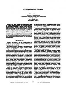
IV. E XPERIMENTAL EVALUATION A. Benefits of incremental and simultaneous solving We now turn to an experimental evaluation of the techniques proposed in this paper. Except where explicitly noted, all experiments were carried out on a machine with dual Intel Xeon E5430 CPUs running at 2.66 GHz using 32 GB of RAM running Linux. The initial experiments are run on instances coming from three nontrivial microcode programs. For these three, MicroFormal was instrumented to dump all instances to files in SMT-LIB format, and produce a log describing how these instances were created. In this paper the programs will be called “program 1”, “program 2” and “program 3”. Table I gives the number of formulae generated in each of these three MicroFormal runs. A test bench has been created which can replay the solver calls in these three runs of MicroFormal, which makes it easy to experiment with different strategies and instrument the system to extract interesting information. In order to emulate the behaviour of MicroFormal, when solving a formula it is first loaded into memory in a separate data structure to avoid measuring the time taking for parsing formulae. From this data structure the MathSAT API is called creating and solving formulae simulating the in-memory usage in MicroFormal as closely as possible without actually running MicroFormal. Apart from the techniques described in this paper, these experiments were performed with MathSAT set up to simply bit-blast and solve the formula using a SAT solver. Since the vast majority of formulas generated by MicroFormal are trivial, this seems to deliver good performance, and this setup should also mean that the techniques described here will also translate to SAT solvers. For the instances taking the most execution time, more aggressive preprocessing techniques can be effective, but the total execution time is dominated by a large number of trivial instances, and the preprocessing normally used in MathSAT seems to be too expensive to be used here. 1) Solving sequences of single formulae: We start by investigating the effect of fixed reset strategies on singleton sets. For these experiments, we solve only singleton sets, skipping over the other calls completely. The result on the three programs are summarized in figure 2. It shows the relative improvement of
Program 1 Program 2 Program 3
10
8
Relative improvement
To solve φi , we solve under the assumption pi . Should it be satisfiable under this assumption, we can easily check which of the other formulae are also satisfied by the same model by checking the truth assignment for the other fresh variables. The algorithm iteratively picks one unsolved formula as a goal and solves under the assumption of the corresponding fresh variable. If it is satisfiable we check if any other unsolved formulae are satisfied by the same model, and discharge all satisfiable formulae.
Program
6
1 2 3
4
2
50
100
150
Reset interval
Fig. 2.
Effect of reset interval on singleton calls
reusing solver information compared to solving each formula in isolation. The horizontal axis shows the reset interval, that is how frequently all learnt information is thrown away. A reset interval of 1 corresponds to solving each formula in isolation. From the figure, it is clear that there is a positive effect of reusing solver information. For program 1 the best improvement is a factor of 4 (at a reset interval of 161), and for program 2 the best improvement is a factor of almost 10 (at reset a interval of 169). Lastly for program 3 the best improvement is a factor of 7.4 (at a reset interval of 99). We can also see that the exact reset frequency is not critical. For program 1 and program 2, there is only a minor difference between different reset intervals above 50. For program 3, the trend is similar but the data appears to be more noisy. This is due to some outliers among the instances to be solved, which are both large and significantly different from any of the others. These cause significant overhead when these instances are retained in the solver and we attempt to solve fresh instances. Performance depends on being able to divest the solver of this irrelevant information as soon as possible, but with a fixed reset interval how quickly this happens is largely due to chance. To avoid this, we will choose a reset interval of 25 for future experiments, which although shorter than what is indicated as the optimal, should on the other hand handle such outliers better. With this reset interval, the improvement for these three programs is a factor of 2.7, 6.7 and 4.9 respectively. To check if reuse of solver information is usable outside of MicroFormal, the technique has also been applied to the instances coming from the SAGE tool [13] (available in SMTLIB under QF BV/sage). Out of 12 sets of instances, a
TABLE II P ERFORMANCE OF THE MSPSAT ALGORITHMS
2000
Reuse
1500
1000
Method
Program 1
Program 2
Program 3
No reuse Reset (25) Reset in-between MSPSAT
104459.86 9104.31 4485.51 6064.98
1722.31 217.13 243.91 278.00
55539.64 5434.52 2694.61 2826.98
●
TABLE III A MPLE PERFORMANCE SUMMARY ( EXECUTION TIMES IN SECS ) ●
500 ● ●● ● ● ●● ●
500
1000
1500
Solver
Type
Median
Mean
Prover
Singleton Non-singleton Ample Singleton Non-singleton Ample
1072.14 389.01 2412.00 98.48 233.25 997.00
2887.13 2264.52 6282.90 289.05 975.24 2183.03
2000
No reuse
Fig. 3. Effect of reusing solver information on SAGE instances. Execution times in seconds
fixed reset strategy of resetting every 25 instances helped in all but two sets. In one of the two, execution time was comparable (332 versus 334 seconds). In the other reusing solver information used 65 seconds versus 11 seconds for solving each instance individually. The added time is taken up in two instances which take considerably more time than the rest. Full results for these sets of instances can be found in figure 3, where total execution time (in seconds) for each set of instances is reported. Although the improvement is not as large as for the three microcode programs seen earlier, there is still a fairly clear improvement, and, indeed this improvement is statistically significant (p = 0.016). 2) Solving sets of formulae: For the cases where MicroFormal generates multiple formulae to solve there are several choices, we will look at a few of them as listed below: 1) Solve them in the same way as single formulae. There might not after all be any need to treat these instances any different from any other. 2) Solve them as with single formulae, but with an infinite reset interval. The motivation is that similarity can be expected to be better within each set than between singleton instances since all instances in a set have been generated at a specific point in symbolic execution. 3) Solve them with MSPSAT. As a baseline, let’s look at the performance when treating each instance as a singleton, disregarding that more than one instance is known a priori. The results are shown in the first row in table II. We can see a significant improvement using MSPSAT over solving each formula individually. For comparison, we also include the execution time when solving all instances reusing solver information using a reset interval of 25, and also when resetting only in between sets of instances. We can see that using a reset interval of 25 gives worse performance than using the MSPSAT algorithm, so there seems to be some value in treating these sets in a special way. For these three programs at least there does however not seem
MathSAT
Standard Dev. 5973.29 4432.13 10316.34 704.25 1751.98 2842.62
to be an advantage with MSPSAT when compared to using a separate solver instance for non-singleton sets which is reset in-between every set. Indeed, the latter technique has a small, but statistically insignificant, advantage over the others. B. Overall impact of MathSAT within Ample As a final experiment the impact of the usage of MathSAT on the Ample tool is evaluated. Ample (Automatic Microcode Path Logic Extraction) is a tool in MicroFormal used for generation of execution paths for dynamic testing, and this will be used for experimental evaluation in this section. For this evaluation 32 different microcode programs have been selected to be representative of small, medium, and large programs. For each, Ample is run with its standard backend engine, the inhouse SAT solver Prover, and with MathSAT. In MathSAT, reusing of solver information was used with a fixed reset frequency of 25, and for non-singleton sets MSPSAT was used. For Prover, singleton sets were solved individually, and nonsingleton sets were solved using the SSAT algorithm. The tool was run on machines with Intel Xeon 5160 CPUs running at 3 GHz and 32GB RAM running Linux, and the execution times of solver calls, other processing, total execution time and memory usage was measured. In these experiments, in no case was memory usage an issue. The results are summarized in table III, which presents the median, mean, and standard deviation values for the total execution time on, respectively, singleton sets of formulae, non-singleton sets (using MSPSAT for MathSAT, SSAT for Prover) and for the total execution time for Ample. The corresponding values, with one point for each of the 32 programs, are plotted in Figure 4. For every program, the performance of MathSAT is better than that of Prover, and for total execution time the improvement is at worst a factor of 1.17, at best a factor of 4.43, and overall the improvement is a factor of 2.88. Not surprisingly, the improvement is statistically significant (p = 9 · 10−9 ). As the experiments on non-singleton sets showed, simply reusing solver information resetting the solver in-between each set may
Solver time (s)
104.5
104
4
● ●
●
●
MathSAT
MathSAT
103
●●
103 ●
● ● ● ● ●● ●● ● ●● ● ●● ● ● ● ● ● ●● ● ●
102
● ● ●
104
●● ●
●● ● ● ● ● ● ● ● ● ● ●● ●
102
●
●
●
● ●
●
103.5
● ●●● ●
● ●
103
● ●
101
●
101
●
●
MathSAT
10
Non−singleton time (s)
●● ●
●
●
●
101
● ●● ●●● ● ● ● ● ● ● ● ●
102.5
●
102
103
104
Prover
101
102
103
104
●
● ●
102.5
Prover
103
103.5
104
104.5
Prover
Fig. 4. Results for each of the 32 programs: (left) total solving times on the singleton sets; (center) total solving times on the non-singleton sets; (right) Ample total execution times.
improve performance further. At the time of writing, this has not been tried on these 32 microcode programs. It should be noted that the difference on non-singleton sets are not necessarily due to the different algorithms (MSPSAT versus SSAT) being used, since two completely different solvers are used for the comparison. V. R ELATED WORK Whittemore et al. [21] describes reusing of learnt clauses in the SATIRE SAT solver. This is an incremental SAT solver which allows the user to retract clauses and add new ones before searching again. To implement this the solver keeps track of the dependencies between learnt clauses and original clauses. If a clause is retracted, all clauses which have been learnt using this clause are also removed. Silva and Sakallah [20] proposed a technique for reusing clauses from one formula to the next in automatic test pattern generation (ATPG) for circuits. In this application a SAT solver is used to try to generate stimuli that expose a particular fault. They notice that some learnt clauses are independent of the current target fault instead depending only on the circuit being studied, and could be reused from one SAT problem to the next. This happens if a learnt clause is derived solely from clauses originating in the circuit. Strichman [19] noticed that in the context of Bounded Model Checking (BMC), certain clauses could be reused from one unrolling to the next. E´en and S¨orensson showed in [11] how learnt clauses could be reused when doing k-induction. This relies on the idea that in this application we are monotonically adding nonunit clauses to the solver, and all unit-clauses can be used as assumptions rather than adding them permanently to the solver. In [14] Große and Drechsler propose to reuse clauses learnt while solving one formula when solving another iff they can be derived from the intersection of the clauses in the two formulae. Babi´c and Hu proposed some simple heuristics to decide if a fact is reusable of not in [5], which allow for reuse of learnt
unit clauses. The only work which considers the idea of reusing all information is the work by E´en and S¨orensson, which is targeted for the case of k-induction where all non-unit clauses in one formula will occur also in the next. For general solving of similar formulae which are not extensions of one another, all previous work concentrate on techniques to compute the relevant parts of the learnt clauses and reuse only those. A. Simultaneous SAT Khasidashvili et al. [16] introduced a technique for solving a set of related formulae using an algorithm they call Simultaneous SAT (SSAT). Given a formula in CNF and a set of proof objectives being literals in this formula, their algorithm is a modification of a normal DPLL-like algorithm. They always keep a particular proof objective as the current goal to satisfy, the currently watched proof objective. At any decision this literal is chosen unless it has already been given a truth value. When the solver finds a model, it checks all other proof objectives and records all that have been satisfied by the model. Then a new currently watched proof objective is chosen among those which has not yet been solved. This is repeated until all proof objectives have been solved. The SSAT algorithm can be seen as a special case of reusing learnt information when all formulae to be solved are known in advance. In contrast to the SSAT algorithm, the MSPSAT algorithm presented in this work doesn’t require any modifications of the underlying solver. Indeed it would be possible to implement using the MathSAT API rather than modifying any part of the solver. VI. C ONCLUSIONS In this industrial case study, we have seen how the introduction of SMT technology can result in increased performance over pure boolean SAT. The experience also demonstrates that a tailored integration within a given verification flow can have a big impact on performance. In particular, reusing
learnt information from solving previous formulae can be very useful, and that in some cases it is possible to achieve good performance without resorting to more complex techniques for reusing information that have been proposed in the past. Simply retaining all information, relevant or not, can provide a significant performance boost with a very low implementation cost and with no added solver complexity. The activity described in this paper has had substantial impact. MathSAT has now been successfully integrated into MicroFormal, and it delivers significantly improved performance over the SAT-based solver previously used. A version of the tool set with MathSAT integrated has been made available to users within Intel with MathSAT available as a commandline option. Using MathSAT, this version has been successfully used for verification of a next generation microarchitecture. In the future, MathSAT will be made the default decision procedure in MicroFormal. Although some improvements have been made to MicroFormal in this case study, the time taken to solve formulae is still considerable compared to the rest of the work of the symbolic execution engine, on average over half the execution time is spent in solving formulae. Therefore, it would be interesting to look for ways of further reducing the time taken to solve instances as well as reducing the number of instances that need to be solved. Listed below are a few possibilities which may be interesting to investigate. Better models: Since MicroFormal is currently capable of storing models for previous formulae, and then use them in a model caching scheme to either avoid future solver calls, or significantly reduce the complexity of future calls, it makes sense to attempt to adapt the models returned from the solver to maximize the utility of this feature. A “good” model in this case is one which models (or can be extended to model) as many future formulae as possible, therefore minimal (or near minimal) models may be interesting. Heuristics for resets: The reset strategy used in this work is a simple strategy with a fixed reset frequency. Although it has been shown to deliver a significant performance improvement, it is still vulnerable to outliers in the sequence of instances. It would be interesting to discover heuristics capable of detecting when irrelevant information stored in the solver is likely to negatively affect performance, and build an adaptive reset strategy around such a heuristic. This should allow for longer reset intervals in the cases where no outliers exists, and further improve performance. A hybrid concrete/symbolic execution engine: One technique which can quickly discover sets of paths in a program is fuzz testing. It might be possible to combine fuzzing with symbolic execution by starting with generating a number of paths with fuzzing, and then extending this set using symbolic execution. The two methods can be interleaved by a technique similar to [13]. Judicial use of fuzzing and concrete execution may in the best case be able to significantly reduce the number of formulae that need to be solved, and taking a closer look at this possibility may be a fruitful avenue of research.
Other possibilities: There are many other possibilities for future improvement. Among them are the following: • Support for uninterpreted functions. MicroFormal abstracts some parts with uninterpreted functions, but currently those are eliminated using Ackermann’s expansion by MicroFormal itself. Passing the original formula on to the solver may improve performance. • Parallelism. There are opportunities for parallelism in MicroFormal. One example would be performing the symbolic execution in parallel exploring several paths simultaneously. ACKNOWLEDGEMENTS This work is supported in part by SRC/GRC under Custom Research Project 2009-TJ-1880 WOLFLING, and by MIUR under PRIN project 20079E5KM8 002. R EFERENCES [1] T. Arons, E. Elster, L. Fix, S. Mador-Haim, M. Mishaeli, J. Shalev, E. Singerman, A. Tiemeyer, M. Y. Vardi, and L. D. Zuck. Formal verification of backward compatibility of microcode. In CAV. 2005. [2] T. Arons, E. Elster, T. Murphy, and E. Singerman. Embedded Software Validation: Applying Formal Techniques for Coverage and Test Generation. Int. Workshop on Microprocessor Test and Verification, 2006. [3] T. Arons, E. Elster, S. Ozer, J. Shalev, and E. Singerman. Efficient symbolic simulation of low level software. In DATE. ACM, 2008. [4] G. Audemard and L. Simon. Predicting learnt clauses quality in modern SAT solvers. In IJCAI. Morgan Kaufmann, 2009. [5] D. Babi´c and A. Hu. Approximating the safely reusable set of learned facts. STTT, 11(4), Oct. 2009. [6] C. W. Barrett, R. Sebastiani, S. A. Seshia, and C. Tinelli. Satisfiability Modulo Theories. In Biere et al. [7]. Part II, Chapter 26. [7] A. Biere, M. Heule, H. van Maaren, and T. Walsh, editors. Handbook of Satisfiability, volume 185 of Frontiers in Artificial Intelligence and Applications. IOS Press, 2009. [8] R. Bruttomesso, A. Cimatti, A. Franz´en, A. Griggio, Z. Hanna, A. Nadel, A. Palti, and R. Sebastiani. A Lazy and Layered SMT(BV) Solver for Hard Industrial Verification Problems. In CAV. 2007. [9] R. Bruttomesso, A. Cimatti, A. Franz´en, A. Griggio, and R. Sebastiani. The MathSAT 4 SMT solver. In CAV. 2008. [10] R. Bruttomesso and N. Sharygina. A Scalable Decision Procedure for Fixed-Width Bit-Vectors. In ICCAD 2009, 2009. [11] N. E´en and N. S¨orensson. Temporal induction by incremental SAT solving. Electronic Notes in Theoretical Computer Science, 89(4), 2003. [12] A. Franz´en. Efficient Solving of the Satisfiability Modulo Bit-Vectors Problem and Some Extensions to SMT. PhD thesis, DISI – University of Trento, 2010. [13] P. Godefroid, M. Y. Levin, and D. Molnar. Automated Whitebox Fuzz Testing. Technical Report MSR-TR-2007-58, Microsoft Research Redmond, Redmond, WA, May 2007. [14] D. Große and R. Drechsler. Acceleration of SAT-Based iterative property checking. In Correct Hardware Design and Verification Methods. 2005. [15] G. Hinton, D. Sager, M. Upton, D. Boggs, D. P. Group, and I. Corp. R The Microarchitecture of the Pentium 4 Processor. Intel Technology Journal, 1, 2001. [16] Z. Khasidashvili, A. Nadel, A. Palti, and Z. Hanna. Simultaneous SATBased model checking of safety properties. In Hardware and Software, Verification and Testing, volume 3875 of LNCS. Springer-Verlag, 2006. [17] S. Khurshid, C. P. as˘areanu, and W. Visser. Generalized symbolic execution for model checking and testing. In TACAS. 2003. [18] J. C. King. Symbolic execution and program testing. Commun. ACM, 19(7), 1976. [19] O. Shtrichman. Pruning techniques for the SAT-Based bounded model checking problem. In CHARME. 2001. [20] J. P. M. Silva and K. A. Sakallah. Robust search algorithms for test pattern generation. In FTCS. IEEE Computer Society, 1997. [21] J. Whittemore, J. Kim, and K. Sakallah. SATIRE: a new incremental satisfiability engine. In DAC. ACM, 2001.