apportionment approach for just-in-time sequencing ... - CiteSeerX

Journal of the Institute of Engineering, Vol. 7, No. 1, pp. 1-14 © TUTA/IOE/PCU All rights reserved. Printed in Nepal. Fax: 977-1-5525830

TUTA/IOE/PCU

APPORTIONMENT APPROACH FOR JUST-IN-TIME SEQUENCING PROBLEM Tanka Nath Dhamala, Ph.D. Prof., Central Department of Mathematics, Institute of Science and Technology, Tribhuvan University Presently: Central Department of Computer Science and Information Technology, TU, Kirtipur.

Gyan Bahadur Thapa Lecturer, Department of Mathematics, Pulchowk Campus, Institute of Engineering, Tribhuvan University

Abstract: The Just-in-Time sequencing of different products is a well-known socio-industrial problem which is supposed to minimize the maximum and total deviations between actual and ideal productions; and the apportionment problem is a socio-political problem which aims to allocate representatives to a state as close as its exact quota. Significant amounts of research have been done in these two problems independently. The relation between them has been studied from last decade. In this article, both problems are addressed with some just-in-time sequencing algorithms and their characterizations via apportionment. Key words: apportionment, divisor methods, algorithms, Just-in-Time sequencing.

1. INTRODUCTION 1.1 Just-in-Time Sequencing Problem Just-in-time (JIT) manufacturing system is a management philosophy based upon the planned elimination of all wastages and on the continuous improvement of productivity; which is done by producing only the necessary amount of necessary products at the right place and at the right time. The goal of JIT system is to minimize the presence of non-value-adding operations and nonmoving inventories in the production line, which results in shorter throughput times, better on-time delivery, higher equipment utilization, better quality products, higher productivity, reduced cycle times, lesser space requirement, lower costs and greater profits. The key behind a successful implementation of JIT process is the reduction of inventory levels at the various stations of the production line; so it is known as lean or stockless production system. The major aim of this system is to satisfy customers for various demands of different

products without holding large inventories and incurring large shortage of the products. The mixed-model JIT sequencing is the problem of determining production sequence of different models of the same product produced on the line by the JIT system, which was developed and perfected by Taiichi Ohno (referred as the father of JIT system) in the Toyota Production System (TPS) around early 1970. This problem is well-studied as a Product Rate Variation (PRV) problem by Kubiak (1993). Some of the basic key elements of JIT production system are group technology, production smoothing, level scheduling, labour balancing, set up time reduction, standard working, visual controls etc. In JIT sequencing (scheduling) environment, products (jobs) that complete early must be held in finished goods inventory till their due dates, while products that complete after their due dates may cause customers to shut down operations. Therefore, an ideal schedule is one in which all products are finished exactly on their assigned due dates.

Journal of the Institute of Engineering

JIT encompasses a much broader set of principles than just those relating to due dates, but scheduling models with both earliness and tardiness penalties do much to capture the scheduling dimension of a JIT approach. The concept of penalizing both earliness and tardiness has spawned a new and rapidly developing line of research in scheduling theory. TPS used the JIT sequencing to distribute production volume and mix of models as evenly as possible over the production sequence (Monden, 1983; Groenevelt, 1993). The JIT sequencing has become a universal and robust concept to balance the two goals of the manufacturing companies: usage goal and loading goal (Monden, 1983; Miltenburg, 1989; Miltenburg et al., 1989). The former maintains a constant rate of usage of all items in the production sequence whereas the latter one smoothes the workload on the final assembly process to reduce the chance of production delays and stoppages. Kubiak (2005) uses JIT sequencing to balance workloads throughout just in time supply chains intended for low-volume high-mix family of products. The purpose of optimal/balanced sequence is to keep the actual production level and the desired production level as close to each other as possible all the time. For more recent literature, we refer to the brief survey of Dhamala and Kubiak (2005). 1.2. Apportionment Problem The problem of how to make a fair division of resources among competing interests arises in many areas of applications in the real world which plays a significant role in decision sciences. A particular problem of fair division having wide application in governmental decision-making is the apportionment problem. The problem of how many representatives should be allotted to a state came in existence since the beginning of the Republican Political system. That is,

2

apportionment problem has its origin in the proportional election system developed for House of Representatives of United States, where each state receives seats in the house in proportion to its population (Balinski and Young, 1982). Moreover, the American Constitution (Article I, Section 2) says that apportionment of representatives to a state should be proportional to its population. Literally, this would mean that some fractional representatives are also to be allotted to the states, which is impossible and meaningless. So some rounding methods must be used to convert the fractions to whole numbers, which are discussed in section 4.2. Though various methods have been used in apportioning the seats in the parliament over the years, often the results seem unfair to many people and bitter disputes have resulted. In section 3, we give a list of surprising paradoxes that happened as a result of using one method or another. Although there is not a single method meeting all the requirements imposed by political needs, a (perfect) apportionment method is supposed to satisfy the following basic properties (see [20]): • Quota Condition: each state should have seats within one of their quotient; e.g., if a state should receive 5.3 representatives, then it can receive 5 or 6 seats. This property is called “satisfying quota”, discussed later as  qi  ≤ ai ≤  qi  . • House Monotonicity: when the total number of representatives (i.e., house size) increases, then any state’s number of representatives should not decrease. • Population Monotonicity: the number of representatives of any state should not decrease as its population increases. Furthermore, any method should not artificially favor large states at the expense of the smaller ones and viceversa.

Apportionment Approach for Just-in-Time Sequencing Problem

3

• Quota Monotonicity: the actual apportionment of any state should not decrease as its quota increases

Zmin = min ∑∑Fi ( xik − kri )

• Minimum Requirement: every state must have at least one representative.

subject to

n

D

n

∑x

ik

• Uniformity: all states should receive the number of representatives by the same formula for representation.

xi( k−1) ≤ xik , i =1, 2,....., n; k =1, 2,....., D

Consider n products to be produced within the specified time horizon, with demands

The constraint

∑d

i

= D . The

i =1

time needed to produce one unit is assumed to be independent on the product and time needed to switch from one product to another is assumed to be negligible. Without loss of generality, it can be supposed that it takes one unit of time to produce one unit of product and thus the time horizon is equal to

D time units. If ri =

di D

with

n

∑

ri = 1 , is

( 4) ( 5)

xiD = di , i =1, 2, ......, n

xik is a non-negative integer

d1 , d 2 ,....., d n ; such that

(3)

=k, k =1, 2,....., D

i=1

2. MODELS OF JIT SEQUENCING PROBLEM

n

( 2)

i =1 k=1

( 3) ensures

(6) that exactly k

units are scheduled in periods1 through k , and ( 5 ) represents the monotone condition. Various scientists have studied above problem via different angles with little-varied objective functions. Miltenburg (1989) suggested following squared and absolute sum deviation just-intime sequencing objectives to be minimized: n

D

fs ( x) = ∑∑( xik − kri )

2

( 7a)

i=1 k=1

i =1

the ideal production rate for the parts of type i , then the scheduling goal for the assembly line is to maintain the total cumulative production of product i to the total production as close to ri as possible. This means exactly kri units of product i should be produced in the periods ( k = 1, 2,...., D ) .

first

k

time

Let xik , i = 1, 2,...., n; k =1, 2,...., D , be the total cumulative production of product i in the time period 1 through k . For a convex symmetric penalty function Fi , i = 1, 2,..., n with minimum Fi ( 0 ) = 0 ; the maximum deviation and sum deviation just-in-time problems are formulated as follows:

Zmax = minmax Fi ( xik − kri ) i ,k

(1)

n

D

fa ( x) = ∑∑ xik − kri

( 7b)

i=1 k=1

He proposed three algorithms: the first one to find the nearest integer point, the second one to test the feasibility of the schedule and the third one (a heuristic) to generate a feasible schedule for the mixed-model JIT production system. Inman and Bulfin (1991) gave an algorithm to minimize the following objective function n

D

f ( y) = ∑∑( yik − tik )

2

(8)

i =1 k =1

where yik and

tik =

2 k −1 2 ri

( i = 1, 2,....., n; k = 1, 2,....., D )

are the times at which k th unit of product i is

Journal of the Institute of Engineering

actually produced and ideally needed respectively. The problem may be interpreted as a single-machine scheduling problem with each unit of product treated as a separate job, where tik is the due date of job ( i, k ) . Steiner and Yeomans (1993) proposed the following maximum deviation objective function to minimize:

g ( x ) = max xik − kri i ,k

( 9)

They reduced the problem into release date/due date decision problem representing as a matching problem in a bipartite graph G = (V1 ∪V2 , E ) , where

V1 = {0, 1,....., D − 1} denotes starting times and V2 corresponds to the copies of each demand. To find a feasible sequence in the release date/due date decision problem is similar to find a perfect matching in bipartite graph G with the additional property that lower numbered copies of a product are always matched to earlier starting times than higher numbered copies. Kubiak and Sethi (1994) minimized the following absolute total deviation objective n

D

h ( x) = ∑∑ Xki − kri

(10)

i =1 k =1

by reducing it into assignment problem, which is efficiently solved, viz. assignment problem with 2 D nodes can be solved in

( )

O D3

time (Papadimitriou and Steiglitz

1982). Tijdeman (1980) studied Chairman Assignment problem providing an algorithm that finds a solution x of the objective function

g ( x) = max xik − kri < 1 i ,k

(11)

with upper bound unity. Later, Jozefowska et al. (2006) vigorously characterized this algorithm with apportionment problem proving that Tijdeman algorithm is quotadivisor method.

4

Our main aim is to link up these JIT sequencing algorithms with the apportionment problem. 3. BASIC CONCEPT OF APPORTIONMENT PROBLEM The apportionment problem is the problem of determining how to divide a given integer number of representatives or delegates proportionally among the given constituencies according to their respective sizes. This is described as follows: Assume that there are s states (or parties) indexed i = 1, 2, ..., s , which are to receive seats of representatives from the house of size h . Suppose every state has a population pi and s

∑

pi = p

is the total population. The

i =1

fundamental problem is to apportion ai seats to state i , where ai ’s must be integers such that s a = h . An ideal apportionment is

∑

i

i =1

assumed to satisfy the equation

pi p

all states, which gives ai =

pi h p

“quota”

=

ai h

for

, called

th

for i state denoted by qi , not

necessarily integer. Since only the integral ai can be assigned to any state, the crucial point is how to handle this problem fairly. One immediate idea is “rounding”: for each state, ideal apportionment should either be rounded down to the next lower integer or rounded up to the next higher integer; but should never exceed these bounds. To this point, Balinski and Young (1975) use the following concept: The ideal apportionment

pi h p

is called “exact quota”

denoted by qi . The largest integer less than or equal to qi is called the “lower quota” li ; the smallest integer greater than or equal to qi is called the “upper quota” ui . An apportionment is said to “satisfy lower quota” if it never gives a state less than its

5

Apportionment Approach for Just-in-Time Sequencing Problem

lower quota of seats, i.e., if li ≤ ai for all i ; to “satisfy upper quota” if it never gives a state more than its upper quota of seats, i.e., if ai ≤ ui for all i ; and to “satisfy quota” if it does both, i.e., if li ≤ ai ≤ ui for all i . This is known as Quota Method of apportionment. Apportionment Paradoxes •

applying Jefferson’s method. For example, in the apportionment based on the 1820 census, New York had a population of 1,368,755, the total US population was 8,969, 878, and the house size was 213. The New York’s quota was thus

q=

1,368, 755 × 213 = 32.503. 8,969,878

But Jefferson method apportioned New York 34 seats.

The Alabama Paradox: An increase in the size of the house can cause a state to lose a seat. This is known as Alabama paradox, appeared while using Hamilton Method of apportionment in 1880 in Alabama State, which received 8 seats from the house size 299, whereas it received only 7 seats from the increased house size 300. This amazing feature (violation of monotonicity) raised some surprise and anxiety in the affected states.

Several apportionment methods are suggested in apportionment literature in different intervals of time by many mathematicians of US and Europe. Some of them are briefly explained here.

•

The Population Paradox: An increase in a state’s population can cause it to lose a seat. This feature is known as population paradox, faced around 1900, while using Hamilton’s method. Still (1979) has defined population paradox as follows: in certain situations, if the population of one state is increased, while holding the other state populations and house size is fixed, then the former state may lose a seat.

This is the simplest method of apportionment proposed by A. Hamilton, which was used to apportion the House of Representatives from 1850 to 1900, under the name of Vinton method of 1850. In this method, each state is given its lower quota of seats. Then the states are listed in order, beginning with the state having the largest fractional remainder (i.e., qi − li ) and continuing on down to the

•

The New States Paradox: Adding new state and increasing house size can cause another state to lose seats, which is known as New States paradox, discovered in 1907 when Oklahoma became a new state. As a new state, Oklahoma received 5 new seats increasing the old house size from 386 to 391. As a result, Maine’s apportionment went up from 3 to 4 and New York’s went down from 38 to 37. But the intent was to leave the number of seats unchanged for the other states.

state with the smallest such remainder. The remaining seats are then assigned one each to the states ranking with the highest fractional part on the list, until the house is full. This method satisfies quota rule, however suffers Alabama, population and New States paradoxes. To avoid these shortcomings, the Divisor methods are developed by E. V. Huntington.

•

The Quota Paradox: Sometimes it may occur that a state receives a number of seats which is smaller than its lower quota or larger than its upper quota, known as Quota paradox and faced while

4. APPORTIONMENT METHODS

4.1 Hamilton’s Method

(Largest

Remainder)

4.2 Divisor (Huntington) Methods All divisor methods, discussed below involve a notion of rounding after finding a suitable divisor d . To use this method, we first look at the exact quota q i = pph . The quantity hp is i

equal to the average number of population represented by each seat in the house. Let

Journal of the Institute of Engineering

do =

p h

. The problem is whether it is

possible to solve the apportionment problem by using a workable value of divisor d , which may not equal to d o , but very near to it. The respective new quotas will be

qi' =

pi d

. The solution for d is not unique;

however the numbers to quotas qi = pi d

pi do

pi d

will be very close

. Interestingly, rounding

might give a different whole number than

rounding

pi do

. The various divisor methods

differ in how they define rounding, which involves the choice of a dividing function D (a ) in each interval of quotients [ a, a + 1] , for

each

non-negative

integer a. Then the result of rounding a number q is  q  if  q  ≤ q < D (  q  ) and  q  if D (  q  )< q ≤  q  . Here, we describe the most important divisor methods.

(i )

Jefferson’s (or Greatest Divisor)

Method: This method rounds down the fractional remainder (i.e., q =  q  ), proposed by T. Jefferson and used from 1790 to 1840. After assigning lower quotas, this method seeks a modified divisor d smaller than the standard divisor d o , and calculates the modified quotas. Then it rounds the modified quotas down to get a new set of minimum quotas. If there are still remaining seats, choose a new modified divisor smaller than the previous one and so on. The dividing function D is DJ (a ) = a + 1 . It does not satisfy quota rule (upper quota violation) and hence favors larger states at the expense of smaller states.

(ii ) Adam’s (or Smallest Divisor) Method: This method rounds up the fractional remainder (i.e., q =  q  ), which was proposed by J. Q. Adam and also advocated

6

by Montana, but was never practical. The dividing function D of this method is DA ( a ) = a . It does not satisfy quota rule (lower quota violation) and hence favors small states.

(iii ) Webster’s

(or Major Fractions) Method: D. Webster corrected Jefferson’s method by rounding the fractional remainder in the usual way (i.e., rounding at the arithmetic mean A between the next lower and next higher whole numbers of the exact quota q ). They simply suggested to round every modified quota down according to the standard rounding rules (i.e., if the fractional part is more than or equal to 0.5 , then round up, otherwise round down). This result of rounding q is defined by q =  q  , if

 q  ≤ q < A and q =  q  , if A ≤ q <  q  ;

where

A = (  q  +  q  )/2. The dividing function D is DW+ ( a ) = a + 12 if a < h (if there are more seats to be awarded) and DW− ( a ) = a − 12 , if a > h (if some seats to be taken away). The state with the largest modified divisor is given additional seat and with the smallest divisor has a seat to be taken away. This process is continued till a = h . It does not satisfy quota rule and does not favor large or small states. It was used in the intervals 1840-1850 and 1900-1941.

(iv) Hill-Huntington’s

(or Equal Proportions) Method: This is the most used method (1941 to present) of apportionment proposed by J. A. Hill and E. V. Huntington around 1911. They argued that states vary so much in size and population. When ratio of their representatives to populations is compared, some of the states are shortchanged compared to other ones. To avoid this defect, instead of rounding the fractional part, this method rounds according

Apportionment Approach for Just-in-Time Sequencing Problem

7

to the geometric mean G between the next lower and next higher whole numbers of the exact quota q . If the modified quota is less than G , then it rounds down, otherwise rounds up. This result of rounding q is

q =  q  , if  q  ≤ q < G

defined by

q =  q  ,

 q  ;

G≤q


aj pj

represents the number

of representatives per person in state i . Ideally the persons of state i have the same number of representatives per person as those ai pi

of state j ; i.e.,

aj

=

pj

, but of course this

generally won’t happen because the numbers ai must be whole numbers. Huntington (1928) made the systematic study of apportionment methods based upon fairness measure, minimizing pair wise measure of inequity (Balinski and Young 1977).

Table 1. Ranking functions and fairness measure of five Huntington methods. Methods

Rank-Index

Fairness measure ai

( p i Jefferson (J) Webster (W)

p a +1

p a+

1 2

p

Hill (H)

a ( a +1)

>

ai (

pj

p 2 a ( a +1) 2 a +1

a j pi

Adams (A)

p a

Thus all divisor methods share the same idea of rounding, but differ in the divisor functions, which are better discussed in table

aj

j

−

ai p j

pj

Dean (D)

j

a

)

− aj)

pi

ai pi

a

aj pj

−1

− apii

ai − a j ( ppij ) 2 by the apportionments obtained for 36 seats for the 6 states.

Journal of the Institute of Engineering

8

Table 2 Apportionment of 36 seats among 6 states State

Population

Exact Quota

Apportionment Methods J

W

H

D

A

A

27,744

9.988

11

10

10

10

10

B

25,178

9.064

9

9

9

9

9

C

19,947

7.181

7

8

7

7

7

D

14,614

5.261

5

5

6

5

5

E

9,225

3.321

3

3

3

4

3

F

3,292

1.185

1

1

1

1

2

1,00,000

36.000

36

36

36

36

36

Two Basic Properties of Huntington Methods: By his test of inequity measure, he described five particular methods, but did not convincingly point out any method as “best”; however his goal was to show that method of Equal Proportions is the best of the five methods, because it is based on the most natural measure of difference, namely the relative difference given by

ai pi

− a

aj pj

min{ pi , i

aj } pj

. The

two basic properties of Huntington methods are “house monotonicity” and “consistency”. If ( p, a ) and ( p ', a ') are tied (i.e., two states having identical populations), then any method M should be “independent” between such states. That is, whenever for some p and h , f i ( p, h ) = a, f j ( p ' h ) = a ' , if

f gives the ( h + 1)

th

seat to state i , then

there should be an alternative solution gε M , identical with f up to h (i.e., th

g h = f h ) that gives the ( h + 1) seat to state j . Any method having this property is called consistent. Moreover, consistency means if ( p, a ) ~ ( p ', a ') , then any two states with populations p and p ' , and apportionments a and a ' are equally deserving in terms of the operation of method M . Theorem 4.2.1 (Balinski and Young, 1977): An apportionment method M is a house

monotone and consistent if and only if it is a Huntington method. 4.3 Parametric Methods A parametric method, denoted by φ δ , is a divisor method φ d based on d ( a ) = a + δ , where 0 ≤ δ ≤ 1 . Various specific parametric methods have been proposed: J. Q. Adams suggested δ = 0 , Condorcet δ = 0.4 , Webster and Sainte-Lague δ = 0.5 and Jefferson and d’Hondt δ = 1 . The parametric methods are cyclic. That is, for two instances of the just-in-time sequencing

D1 = d1 , d 2 ,....., d n and D2 = kD1 = kd1 , kd 2 ,....., kd n , the sequence for D2 is obtained by k repetitions of the sequence for problem D1 . Note that, as δ increases from 0 to 1 , seats being “given-up” by the smaller states in favor of the larger states. This is characterized by the following lemma (Balinski and Ramirez, 1999): Lemma: A parametric method φ α gives-up to another parametric method φ β iff α < β . Thus parametric method φ δ is most favorable to smaller states with δ = 0 and most favorable to larger states with δ = 1 . The fundamental properties of this method are: Scale-invariancy:

Apportionment Approach for Just-in-Time Sequencing Problem

9

φ ( p, h ) = φ ( λ p, h ) , for Exactness: and

∑p

i

p is

if

= h,

all λ > 0 ;

then

integer

p is

the

valued unique

i

solution φ ( p, h ) = p ; Anonymity: solutions depend only on the values of the data, not on the order in which the data is presented. A method φ is balanced if aεφ ( p, h ) and

pi = p j implies ai − a j ≤ 1 . Lemma: A consistent, exact and anonymous method is balanced A method φ

is said to be cyclic if

aεφ ( p, h )

and

p integer

implies a + pεφ ( p, h + ps ) , for an example, Hamilton method is cyclic. Theorem 4.3.1 (Balinski and Ramirez 1999): A divisor method φ is parametric iff it is cyclic.

satisfies three requirements: satisfying quota, house monotonicity and mathematical consistency. Still (1979) defined a class of new apportionment methods (including Quota method) that are also house monotone and satisfy quota. The first characteristic of Still’s method is that all of them are defined recursively as follows: in the trivial case of a house of size 0 , all states are assigned 0 seats. At all larger house sizes, the apportionment is the same as at the next lower house size, but with the additional seat assigned to one of the states according to specified rules. This sequential procedure assures house monotonicity. The second characteristic is the use of eligibility set: a set of those states which are eligible to receive the additional seat, denoted by E ( h) , where

h is house size. The eligibility set E ( h ) at any house size h > 0 consists of all states i that satisfy the following tests:

4.4 Quota Methods Balinski and Young proved that there is no Huntington method that satisfies quota; only the method of smallest divisor satisfies upper (ceiling of exact representation) and only Jefferson’s method satisfies lower quota (floor of exact representation). They devised a method, called Quota method, which avoids both the Alabama paradox and Quota paradox (Balinski and Young, 1975). This is the refinement of the Huntington method. Instead of comparing all the states in the minimization of shortchangedness, only states that are eligible to receive a seat or to lose a seat are considered. Eligibility means that they won’t exceed upper quota or won’t go below lower quota upon receiving or loosing a seat. However, this method is biased favoring large states, since Jefferson’s method is used to compare the states. To avoid this flaw, in the uniqueness proof for their method, Balinski and Young proved that Quota method is the only method which

The upper quota test: the state i satisfies the upper quota test if ai ( h − 1) < ui ( h ) , where ui is the upper quota. The lower quota test: let hi be the house size at which state i first becomes entitled to obtain the next seat, i.e., hi is the smallest house size h ' ≥ h at which the lower quota of state i is greater or equal to ai ( h −1) or n a  hi =  i( hp−i1)+1 ∑ pi  . i =1  

For

each

house

interval h ≤ g ≤ hi ,

size

g in

the

define

si ( g , i ) = ai( h −1) + 1 (the number of seats that state i has in a house of size h before an additional seat is assigned +1); for j ≠ i ,

si ( g , i ) = max{ai ( h − 1) , lg ( h )}. If there is no house size g , h ≤ g ≤ hi , for which

Journal of the Institute of Engineering

∑ s ( g, i ) > g , j

then state i satisfies the

j

lower quota test. The eligibility set E ( h ) consists of all states which may receive the available seat without causing a violation of quota either at h or any larger house size. That is, E ( h ) = {i th state: i th state passes the upper and the lower quota tests}. Still (1979) proved that the eligibility set E ( h ) contains at least one state, for h > 0 ; and all apportionment methods in the class are house monotone and satisfy quota. The states from E ( h ) can be chosen in various ways, for example

( i ) by

using ranking

functions (population, land area, alphabetical order, percent of minorities or women in population etc). ( ii ) by using random selection.

( iii ) by

using

quota-divisor

methods, which are based on divisor methods. The only difference is that the states in quota divisor methods must be from E ( h ) . This algorithm is defined as follows:

(i )

M ( p,0 ) = 0

( ii )

if aε M ( p, h ) and k , iε E ( h ) pk d ( ak )

satisfies

= max d (pai i ) , i

then

bε M ( p, h + 1) with bk = ak + 1 for i = k and

bi = ai for i ≠ k . It is difficult to find a perfect apportionment method. Even the quota methods for congressional apportionment are non-unique (Mayberry, 1978). In this regard, Balinski and Young (1982) give the following Impossibility Theorem: Theorem 4.4.1: There are no perfect apportionment methods. Moreover, it is

10

impossible for an apportionment method to be population monotone and stay within the quota at the same time for any reasonable instance of the problem

( s ≥ 4 and h ≥ s + 3) . 4.5 Balanced Method Roman Shapiro [20] discovered balanced method, which minimizes the advantages of large states over small states in the Jefferson’s method. For each state i , this method uses the following formula to find the apportionment:

ai =

pi h ε , where ∆ = pi p (1 + ∆ ) 1 + pC

Here h = house size, pi = population of p= total population, state i , C = coefficients to balance out the effect of large state. The exact quota

pi h p

of state i is

multiplied by a proportion that is somewhat bigger than one. The epsilon ( 0 ≤ ε ≤ 1) is balancing out the effect of truncation, but favoring large states. To reduce this effect of ε for large states and to satisfy upper quota, there is another number C , balancing that effect and making sure that the results satisfy quota. This method satisfies quota and uses the same formula for representation of all states. However, it favors small states and admits the Alabama paradox. Compared to other methods, this method provides a better alternative if someone would wish to give an advantage to smaller states and stay within quota. This is the reason for the results of the balanced method to be similar to the results of the method of Smallest Divisor (Adam’s method). 5. LINK BETWEEN JIT SEQUENCING AND APPORTIONMENT PROBLEMS Many authors have stirred up on the connection of JIT sequencing (PRV) problem

11

Apportionment Approach for Just-in-Time Sequencing Problem

with apportionment problem. Bautista et al. (1996) have established the relation between JIT sequencing and apportionment problems, stating that the former problem can be seen as a constrained sequential apportionment problem. The monotone condition of PRV problem is equivalent to house monotonicity in apportionment. They first indicated that the algorithm of Inman and Bulfin (1991) is the Webster divisor method of apportionment, which is the fundamental socio-political question. Subsequently, Balinski and Shahidi (1998) proposed a strong approach to JIT sequencing via axiomatics, originally developed for the apportionment problem. The axiomatic method of apportionment depends on some socially desirable and crucial characteristics, such as satisfying quota, house and population monotonicity etc, which must be satisfied for the solution of apportionment problem. However, the famous Impossibility Theorem of Balinski and Young puts a limitation that there are no perfect apportionment methods satisfying all properties. Balinski and Ramirez (1999) vigorously characterized PRV problem in terms of parametric methods of apportionment and rounding as well. Recently, Józefowska et al. (2006) lucidly characterized some of the algorithms of JIT sequencing via apportionment theory. They classified various apportionment methods in a very clear way and linked JIT sequencing algorithms with apportionment via suitable pictorial representation too. Their transformation of two problems is remarkable: product (model) i corresponds to state i , the demand d i for model i corresponds to population pi of state i , the

number of products n ⇔ number of states product i ⇔ state i demand d i for product i ⇔ population pi of state i position in sequence k ⇔ size of house h for a house of size h , xik ⇔ apportionment n

ai to state i total demand D = ∑ d i ⇔ i =1 s

total population p =

∑p

i

i =1

6. SEQUENCING ALGORITHMS AND APPORTIONMENT METHODS Inman-Bulfin (IB) algorithm: Bautista et al. (1996) observed that IB algorithm (1991) to minimize the sum deviation objective function (8) is equivalent to Webster divisor method. The optimal value is obtained by applying earliest due date (EDD) algorithm taking tik as due dates. In IB algorithm, the units are sequenced

according to

increasing order of the values Webster’s

method

apportionment is

the

2 pi 2 ai − 1

2 ki − 1 2 ri

the

and in

rank-index

for

, thus both procedures

are equivalent, and hence Webster optimizes

( 8) with due dates tik

i

=

2 ki − 1 2 ri

.

Steiner-Yeomans (SY) algorithm: Steiner and Yeomans (1993, 1994) proposed a graph theoretic polynomial time algorithm to minimize the maximum deviation objective function (9) based on the following theorem with target value T. Theorem 6.1: A just-in-time sequence with min max xik − kri < T exists iff there exists ik

cumulative production xik of i product in

a sequence that associates the j th copy of

period k corresponds to the number a i of

product i in the interval  E ( i, j ) , L ( i, j )  , where

th

seats apportioned to state i in a house of size h . More precisely, this transformation is as follows:

Journal of the Institute of Engineering

E ( i, j ) =  r1i ( j − T ) 

and

*

are the earliest and latest starting times respectively of j th copy of i th product in the final production sequence. The SY algorithm tests the values of T from the following list in ascending order D − d max D

,

D − d max D

+1

, .....,

j th copy of product i to the

assigning

k th period. If k < Z ij ( j th copy is produced

L ( i, j ) =  r1i ( j − 1 + T ) + 1

T=

12

D −1 D

too early), then the excess inventory cost ψ ijl are incurred in periods from l = k i* j

i* j

l = Z − 1 . If k = Z , then j copy of product i is produced in its ideal position

C ijk = 0.

and

*

to l = k − 1 . Thus the sequencing cost of j th copy of the product i in period k is calculated by the following formula. *

Z ij −1

ik

If T ′ is feasible, then all T , T ′ ≤ T ≤ 1 −

Theorem 6.2: The SY algorithm with T , T * ≤ T < 1 and a tie L ( i, j ) = L ( k , l ) between i and k broken by choosing the

( j − 1 + T ) , r1 ( l − 1 + T )} k

is a quota-divisor with d ( a ) = a + T . Moreover, SY algorithm is parametric method with δ = T .

method

∑ψ

i jl

*

if k < Z ij

,

l =k

C ijk =

*

if k = Z ij

0, k −1

∑ψ

C ijk =

i jl

,

*

if k > Z ij ,

*

l = Z ij

ψ ijl = j − lri − j − 1 − lri ,

where

(i, j) εI ={(i, j) :i =1,.....,n; j =1,.....,di} , i =1,....., D The authors proved that an optimal solution to minimize (10 ) subject to ( 3) to ( 6 ) , can easily be obtained from any

a

quota-

Kubiak-Sethi (KS) algorithm: Kubiak and Sethi (1991, 1994) and Kubiak (1993) nicely reduced the objective function (10) under the constraints ( 3) to ( 6 ) into equivalent assignment problem. The key idea is as follows: For each product i , the ideal position is calculated by the formula

Z ij =  22jr−i 1  , n = 1, 2,....., n and j = 1, 2,......, d i . Let C ijk be the cost of *

C ijk =

1 D

are feasible as well. The smallest feasible T is denoted by T * and referred to as optimum. Józefowska et al. (2006) proved that SY algorithm is a quota-divisor method of apportionment providing the following theorem.

1 ri

is

cost ψ ijl are incurred in periods from l = Z ij

min max xik − kri Z ij ( j th copy

If

produced too late), then the excess shortage

.

Brauner and Crama (2004) proved that at least one of these values is feasible. So we have

one with min

to

th

optimal solution of the following assignment problem: D

minimize

∑ ∑ε C

i jk

x ijk

k =1 ( i , j ) I

subject to

∑ε

(i , j )

x ijk = 1, k = 1, 2, ....., D I

D

∑x

i jk

= 1,

( i, j ) ε I

k =1

xijk = 0 or 1, k = 1, 2, ....., D, ( i, j ) ε I ,

Apportionment Approach for Just-in-Time Sequencing Problem

13

where

xijk =

{

1, if ( i , j ) is assigned to period k 0, otherwise .

Józefowska et al. (2006) characterized KS algorithm based on the following three lemmas. Lemma 1. The KS algorithm does not stay within the quota. Proof: Corominas and Moreno (2003) observed that no solution minimizing the Kubiak-Sethi PRV problem (10 ) subject to constraints ( 3) to ( 6 ) stays within the quota, for instance of n = 6 products with their d1 = d 2 = 23 demands being and

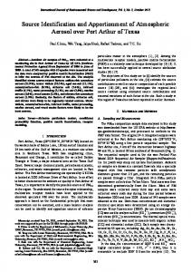
Figure 1. Characterization of JIT sequencing algorithms and apportionment methods.

d 3 = d 4 = d 5 = d 6 = 1. Since KS algorithm minimizes (10 ) , this proves the lemma.

7. CLOSING REMARKS

Lemma 2. The KS algorithm is house monotone. It is obvious due to constraint ( 5 ) .

Though universally accepted independent solution of JIT sequencing problem is not available till the date, there are various approaches to handle this problem, some of them, for example, are single machine scheduling, assignment, Chairman assignment, dynamic programming, apportionment etc. We have tried to link up the JIT sequencing problem with apportionment problem. Assigning exact quota as integer number of seats from a fixed

Lemma 3. The KS algorithm is not uniform, and hence is not population monotone. To sum up, the authors have classified various apportionment methods and characterize the JIT sequencing algorithms in the following quaternion Venn-diagram, where notational conventions are as follows: HM = house monotone methods, NHM = not house monotone methods, Q = quota methods, NQ = not quota methods, Un = uniform methods, Dv = divisor methods, QD = quota divisor methods, P = parametric methods, Still = Still’s methods, J = Jefferson, W = Webster, A = Adams, H = Hill, D = Dean, Ht = Hamilton method, T = Tijdeman algorithm, SY = SteinerYeomans algorithm, KS = Kubiak-Sethi algorithm, IB = Inman-Bulfin algorithm.

house size h to a state satisfying

n

∑a

i

=h,

i =1

itself is really a difficult real life problem. Among all divisor methods, Hill-Huntington method is near to ideal apportionment, which is suitable approach to JIT sequencing problem. While studying the existing literatures, we can say that both problems have similar nature and hence they can be investigated jointly. 8. ACKNOWLEDGEMENT We are indebted to our respected Prof. Dr. Shankar Raj Pant for his continuous inspiration and support in our study.

Journal of the Institute of Engineering

REFERENCES

[1]

M. Balinski and H. P. Young (1974), A New Method for Congressional Apportionment, Proc. Natl. Acad. Sci. USA 71, 4602- 4606. [2] M. Balinski and H. P. Young (1975), The quota method of apportionment, American Mathematical Monthly 82, 701-729. [3] M. Balinski and H. P. Young (1977), On Huntington method of apportionment, SIAM Journal on Applied Mathematics (Part C) 33, 607618. [4] M. Balinski and V. Ramirez (1999), Parametric methods of apportionment, rounding and production, Mathematical Social Sciences 37, 107122. [5] M. Balinski and N. Shahidi (1998), A simple approach to the product rate variation problem via axiomatics, Operations Research Letters 22, 129135. [6] J. Baustista, R. Companys and A. Corominas (1996), A Note on the relation between the Product Rate Variation Problem and the Apportionment problem, JORS 47, 1410-1414. [7] N. Brauner and Y. Crama (2004), The maximum deviation just-in-time scheduling problem, Discrete Applied Mathematics 134, 25-50. [8] T. N. Dhamala and W. Kubiak (2005), A Brief Survey of Just-in-Time Sequencing for Mixed-Model Systems, International Journal of Operations Research 2, 38-47. [9] H. Groenevelt (1993), The JIT Systems, In: Graves, S. C., Rinnooy, K., Zipkin, P.H., editors, Handbooks in Operations Research and Management Science Vol. 4, North Holland. [10] E.V. Huntington (1928), The Appointment of Representatives in Congress, Transaction of the American Mathematical Society, Vol. 30, No. 1, pp 85-110.

14

[11] R. R. Inman and R. L. Bulfin (1991), Sequencing JIT Mixed-Model Assembly Lines, Management Science 37, 901-904. [12] J. Jozefowska, L. Jozefowski and W. Kubiak (2006), Characterization of Just-in-Time Sequencing via Apportionment, A chapter of Book Series in OR and Mgmt. Science. [13] W. Kubiak and S. P. Sethi (1994), Optimal Just-in-Time Schedules for Flexible Transfer Lines, The International Journal of Flexible Manufacturing Systems 6, 137-154. [14] W. Kubiak (1993), Minimizing variation of production rates in just-intime systems: A Survey, European Journal of Operational Research 66, 259-271. [15] W Kubiak (2005), Balancing MixedModel Supply Chains, Chapter 6 in Volume 8 of the (GERAD) 25th Anniverssary Series, Springer. [16] J. P. Mayberry (1978), Quota methods for congressional apportionment are still non-unique, Proc. Natl. Acad. Sci. USA 75, 3537-3539. [17] J. Miltenburg (1989), Level Schedules for Mixed-Model Assembly Lines in Just-in-Time Production Systems, Management Science 35, 192-207. [18] N. Moreno and A. Corominas (2003), Solving the minsum PRV Problem as an Assignment Problem, 27 Congreso Nacional de Estadistica e Investigacion Operativa Lleida, 8-11. [19] Y. Monden (1983), Toyota Production Systems, Industrial Engineering and Management Press, Norcross, GA. [20] R. Shapiro, Method of Apportionment (online), Apportionment of Representatives in the United States Congress House of Representatives and avoiding the ‘Alabama Paradox’. [21] G. Steiner and S. Yeomans (1994), A Bicriterian Objective for Leveling the Schedule of Mixed-Model, JIT Assembly Process, Mathematical Computer Modeling 20, 123-134.

15

Apportionment Approach for Just-in-Time Sequencing Problem

[22] G. Steiner and S. Yeomans (1993), Level Schedules for Mixed-Model Just-in-Time Process, Management Science 39, 728-735. [23] R. Tijdeman (1980), The Chairman Assignment Problem, Discrete Mathematics 32, 323- 330.

[24] C. H. Papadimitrou and K. Steiglitz (2003), Combinatorial Optimization: Algorithms and Complexity, Prentice Hall of India, Pvt. Ltd. [25] J. W. Still (1979), A Class of New Methods for Congressional Apportionment, SIAM Journal on Applied Mathematics 37, 401-418.