Proceedings CPAIOR’02
Approaches to Find a Near-minimal Change Solution for Dynamic CSPs Yongping Ran University Maastricht Department of Computer Science P.O. Box 616,6200 MD Maastricht, NL. email:
[email protected] Nico Roos University Maastricht Department of Computer Science P.O. Box 616,6200 MD Maastricht, NL. email:
[email protected] Jaap van den Herik University Maastricht Department of Computer Science P.O. Box 616,6200 MD Maastricht, NL. email:
[email protected] February 28, 2002 Abstract A Dynamic Constraint Satisfaction Problem (DCSP) is a sequence of static CSPs that are formed by constraint changes. In this sequence, the solution of one CSP may be invalidated by one or more constraint changes. To find a minimal change solution for that CSP with respect to the solution of the previous related CSP, a Repair-Based algorithm with Arc-Consistency (denoted as RB-AC in [4]) has been developed. However, when a new CSP is formed by adding or changing several n-ary (n ≥ 2) constraints, using RB-AC to find a minimal change solution is much harder than using a constructive algorithm to generate an arbitrary solution from scratch. The constraint propagation techniques integrated in RB-AC do not reduce its time complexity. This paper proposes two approximate algorithms to reduce the time complexity of RB-AC by relaxing the criteria of an optimal solution. The experimental results show that one of the proposed algorithms performs quite well in terms of approximation of a minimal change solution within a limited period of time.
Keywords: Dynamic CSP, algorithm, minimal change, optimal solution, local search, approximation, randomize, restart.
1
Introduction
Many AI problems can be modeled as Constraint Satisfaction Problems (CSPs). In practice, a CSP problem definition may change over time because of the environment, the user’s preference or an agent’s behavior in a distributed system (e.g., a machine breakdown or a late delivery of material in a job shop). Each separate change may result in a new CSP. The sequence of such CSPs is denoted as a Dynamic CSP (DCSP) [1]. In a Dynamic CSP, a valid solution of one CSP may not be a solution of the next CSP invoked by the new situation. Hence, a new solution must be generated for that CSP. To get a solution for such CSP, it is always possible to solve it from scratch. However, any solution obtained in this way might be quite different from a previous one. In practical situations, large differences between successive solutions are often undesirable. Recently, H.E. Sakkout et al. [5, 2] proposed an algorithm called “Probe Backtrack Search” to minimally reconfigure schedules in response to a changing environment. They use a very close integration of constraint-directed search with linear programming optimization. However, their solution methods are designed in particular on solving Kernel Resource Feasibility Problems (KRFP). The constraints, optimization function and variable domains in KRFP are quite specific with respect to general DCSPs. For instance, the algorithm introduced in [5] conducts search in two interleaved phases, i.e., resource feasibility phase and temporal optimization phase. In most cases, it is impossible to categorize the constraints of a general DCSP into resource and temporal constraints. So, their solution methods may not be applicable for a general DCSP. In 1998, R.J. Wallace and E.C. Freuder [7] proposed an algorithm to generate solutions that are expected to remain valid after constraint changes in a DCSP. This approach is based on the assumption that the successive changes in DCSP are temporary and tractable. However, when unexpected events occur, the assumptions may no longer be well grounded. As the authors pointed out, in the cases of constraint addition, it is quite complicated to track down the changes directly. Thus, that approach may become too costly to be viable [8]. Somewhat longer ago, Verfaillie and Schiex [6] proposed an algorithm that reuses the solution of a previous CSP to solve the new CSP. They start from selecting an unassigned variable (or a variable that is in the violated constraints) and assign it a value. Subsequently, they apply a constructive CSP solution method, such as backtracking search with forward checking. The new assignment for the selected variable must be consistent with a set (V 1) of assigned and fixed variables. However, it may be inconsistent with the variables in a set (V 2) of assigned and not fixed variables. When this happens, they unassign a variable that is inconsistent with the new assignment from V 2 and then repeat the previous steps. Clearly, the set of variables that will be assigned a new value is rather arbitrary. It depends on choices of new values to the unassigned variables. There is no way to guarantee that this will result in a nearby solution. The solution stability was carried out by fixing the value assignments of a set of variables in the solution of the previous CSP. Of course, a drawback for a general DCSP is that it is hard to predict which value assignments of variables should be fixed in a dynamic environment. Moreover, in some specific application domains carrying out the solution maintenance by
fixing the value assignment of a set of variables is limited. In other application domains, the objective to maintain as many as possible value assignments of variables equal to the old ones is almost prerequisite. For instance, assuming that the task is scheduling people working in a hospital and that someone becomes ill, then too many changes to the old schedule may result in many night shifts, weekend shifts and corresponding compensation days of all employees. To cope with these application demands, a new algorithm RB-AC was proposed in our earlier paper [4]. Instead of creating a completely new solution from scratch, RB-AC uses the solution of the previous CSP (seen as an infringed solution of the current CSP) and systematically searches the neighborhood of the infringed solution by combining local search with constraint propagation to find a minimal change solution for the current CSP, i.e., it modifies the minimal number of value assignments in the infringed solution to satisfy all constraints in the current CSP. In the context of this paper, the notion ‘distance’ is used to denote the number of different assignments between solutions of two CSPs. Consequently, the optimal solution of the current CSP is defined as the solution that has the shortest distance to the solution of its immediate predecessor CSP. As indicated in [4], RB-AC theoretically can find an optimal solution for each CSP (if a solution exists) in a DCSP. Moreover, if the new CSP is the result of adding a unary constraint, the time consumption of RB-AC is not much higher than solving the new CSP from scratch. However, if several n-ary (n ≥ 2) constraints are added to the CSP, and this happens quite often in a practical situation, the time consumption of RB-AC increases drastically. To solve these CSPs, RB-AC may not find an optimal solution in a reasonable period of time. The reason is that the search efficiency of RB-AC is affected when we intend to obtain an optimal-solution stability, i.e, maintaining as many as possible value assignments. Hence, we face an important trade-off between search efficiency and solution optimality. By examining the RB-AC algorithm more closely, we found that a significant portion of the search effort in RB-AC was consumed by additional overhead that the constructive algorithm AC1 does not have. In this paper, we provide an analysis of the additional overhead in RB-AC. Then, we deal with the approaches that balance the search efficiency and solution optimality in such a way that a part of the additional overhead is avoided and a near-optimal solution is obtained within a reasonable period of time. The paper is organized as follows: Section 2 presents the CSP model, the RB-AC algorithm and an analysis of its time complexity. Section 3 presents our approximate algorithms; various limitations and extensions to the algorithms are discussed. Section 4 deals with experimental results, and Section 5 provides some conclusions.
2 2.1
Definitions and Descriptions The CSP model
Below, we provide three definitions on (1) a CSP, (2) a complete assignment, (3) a solution of a CSP. Definition 1 A constraint satisfaction problem (V, D, C) involves a set V = {v 1 , v2 , · · · , vn } of n variables, a set of domains D = {Dv1 , Dv2 , · · · , Dvn } and a set C of constraints. A 1 In this paper, AC stands for a backtracking search algorithm that applies arc-consistency on the yet unassigned variables when the algorithm starts and when a variable has been assigned a value.
constraint cvi1 ,···,vik : Dvi1 × · · · × Dvik → {true, f alse} is a mapping to true or false for an instance of Dvi1 × · · · × Dvik . S Definition 2 A complete assignment a : V → D for a CSP (V, D, C) is a function that assigns values to variables. For each variable v ∈ V, a(v) ∈ D v . S Definition 3 For a CSP (V, D, C), let a : V → D be a complete assignment. Then a is a solution of the CSP iff for each cvi1 ,···,vik ∈ C: cvi1 ,···,vik (a(vi1 ), · · · , a(vik )) = true. Following the formal definition of CSP and its solution, we briefly describe the RB-AC algorithm in the next subsection.
2.2
Description of RB-AC
Given an instance of CSP (V, D, C) and an array a containing a complete assignment for all variables in V . The RB-AC algorithm presented in Figure 1 solves the CSP by calling the procedure solve(V, D, C, a). Below, we first explain the procedure solve and then explain the procedures f ind and assign. The procedure solve starts on identifying the current problem. Since a is presumed to be an infringed solution for the given CSP (V, D, C), some of the constraints are violated. Consequently, at least some of the variables involved in these violated constraints need to change their value assignments. The set X (Figure 1, line (1)) collects these variables. Moreover, constraint propagation is applied on the original domains of all variables to determine the variables that must be assigned a new value, i.e., the variables of which the current value assignments of a lay outside their domains after constraint propagation. These variables are collected in the set U (Figure 1, line (2)). As a result, the new set X, i.e., the set of all variables which may be assigned a new value (Figure 1, line (3)), is updated2 . Thereafter, the initial number of variables n that are to be assigned a new value, is set at max(1, |U |) (Figure 1, line (4)). If X is not empty and n ≤ |V |, the procedure solve calls the procedure f ind(V, 1, U, X, ∅). If the first call of f ind(V, 1, U, X, ∅) does not return success, then the variable n (Figure 1, line (5)) the maximal number of variables that may be assigned a new value is re-determined, and the procedure solve iteratively calls f ind(V, 1, U, X, ∅) until it returns success or n > |V |. RB-AC selects the appropriate variables in the procedure f ind(F, i, U, X, Y ). If U 6= ∅, f ind selects a variable from U and then calls the procedure assign. Otherwise, it selects a variable from the set X and then calls the procedure assign. If the call of assign fails and the variable is selected from the set X, f ind will try another variable in the set X until X becomes empty or one call of assign returns success. The selected variable is assigned a new value in the procedure assign(v, F, i, Y ). Subsequently, the sub-procedure constraint-propagation(F) enforces arc-consistency on the variables in the set F that have not been assigned a new value yet. Whether more variables need to be assigned a new value is determined by recalculating the sets U (Figure 2 By first handling the variables in the set U that must be assigned a new value, we might avoid to try multiple choices from the set X and thus improve the search efficiency [4].
Procedure solve (V, D, C, a) X:=conflict var(C, a); constraint-propagation (V ); U := {v ∈ V | a[v] ∈ / D[v]}; X := X ∪ U ; n := max(1, |U |); u := |V |; if X = ∅ then return success; while (n ≤ |V |) do if (f ind(V, 1, U, X, ∅) = success) then return success; n := max(n + 1, u); u := |V |; end; return f ailure; end.
end; end; return f ailure; end.
(1) (2) (3) (4)
Procedure assign(v, F, i, Y ) save(D[v], a[v]); D[v] := D[v] − {a[v]}; while (D[v] 6= ∅) do d1 :=select-value(D[v]); D[v] := D[v] − {d1 }; a[v] := d1 ; save(D[v ∗ ] |∀v ∗ ∈ F ); constraint-propagation(F ); if (∀v ∗ ∈ F, D[v ∗ ] 6= ∅) then U := {v ∗ ∈ F | a[v ∗ ] ∈ / D[v ∗ ]}; (9) (10) X := U ∪ conflict var(C, a); j := max(1, |U |); if (X = ∅) then return success; else if (i + j ≤ n ∧ U ∩ Y = ∅) then return find(F, i + 1, U, (F ∩ X) − Y, Y ); else u := min(u, i + j); (11) end; restore(D[v ∗ ] |∀v ∗ ∈ F ); end; restore(D[v], a[v]); return f ailure; end;
(5)
Procedure find(F, i, U, X, Y ) if (U 6= ∅) then v :=select-variable(U ); if(assign(v, F − {v}, i, Y ) = success) then return success; else while (X 6= ∅) do (6) v :=select-variable(X); X := X − {v}; if(assign(v, F − {v}, i, Y ) = success) then return success; Y := Y ∪ {v}; (7) F := F ∪ {v}; (8)
[
conflict var(C, a) := cv i
1
,···,vi
k
∈C,cvi
1
,···,vi
k
(a(vi1 ),···,a(vik ))=f alse
Figure 1: RB-AC algorithm.
{vi1 , · · · , vik };
CSP(V,D,C) v2 1 2
v1 2 3
1 2 v3
3 4 v4
solution: a[v1]=2 a[v2]=1 a[v3]=1 a[v4]=3
Ci,j=“not equal” v1 v2 2 1 3 2
1 2 v3
New solutions after a[v1]=3 a[v2]=2 a[v3]=1 a[v4]=4 AC solution
3 4 v4 adding a constraint a[v1]=3 a[v2]=2 a[v3]=1 a[v4]=3 RB-AC solution
Figure 2: Simple example of RB-AC execution. 1, line (9)) and X (Figure 1, line (10)). If X = ∅, the problem is solved and assign returns success. Otherwise, assign(v, F, i, Y ) either recursively calls the procedure f ind (when i < n) or updates u (Figure 1, line (11)) and backtracks to assign another value for the selected variable (when i = n). If the set X is still not empty after the domain of the selected variable has become empty, assign will returns failure. Since the newly calculated set X usually overlaps with the previously calculated set X, we could say that RB-AC investigates subsets of a set X. In order to avoid investigating the same subset of X twice, e.g. first by selecting vi and then vj and second by selecting vj and then vi , the set Y is used. In summary, RB-AC finds an optimal solution by systematically searching the neighborhood of the infringed solution with an iterative deepening approach. If RB-AC fails to find a solution through an exhaustive search with changing the value assignments of n variables, it tries to change the value assignments of n0 variables with n0 > n. If this fails too, it takes n00 variables with n00 > n0 , and so on. Let us show a simple example to explain the ideas behind the RB-AC algorithm. Simple example The left graph of Figure 2 depicts a constraint graph of a CSP instance (V, D, C), where V = {v1 , v2 , v3 , v4 }, Dv1 = {2, 3}, Dv2 = {1, 2}, Dv3 = {1, 2} and Dv4 = {3, 4} are the corresponding domains; and where each line linked between two variables denotes a not equal constraint. Let a(v1 ) := 2, a(v2 ) := 1, a(v3 ) := 1 and a(v4 ) := 3 be a complete assignment satisfying all constraints. Now assume that a binary constraint (not equal ) has been added between v2 and v3 as showed in the right graph of Figure 2. Consequently, the values assigned to the variable v2 and v3 are not consistent
with this new added constraint. Hence X := {v2 , v3 }. At least one variable in the set X that violates the new added constraint must change its value. Since U = ∅, the initial n is set to 1 (n := 1). Next, the algorithm changes the value assignment of a variable in X. If the algorithm selects v2 from X and assign it a new value a(v2 ) := 2, the new added constraint is satisfied. However, the constraint between v1 and v2 is violated. After applying arc-consistency, the current value assignment of v1 is no longer in its domain, and v1 will be added to U . This means that the value assignment of v1 has to be changed too. Since n = 1, it is not allowed to change two value assignments in this iteration. Thus, the algorithm restores the initial value assignment of v2 and initial domain of v1 , selects v3 from the set X and assigns it a new value a(v3 ) := 2. The same situation arises when changing the value assignment of v2 . As a result, all possibilities of changing one value assignment are exhaustively tried without success. Therefore, more variables have to change their value assignments. In order to find the most nearby solution such that all constraints are satisfied, a systematic exploration of the search space is required. In other words, if the algorithm fails to find a solution by changing the value assignment of one variable, it must look at changing the value assignments of two variables. If this fails too, the algorithm takes three variables, and so on. This process is the well-known iterative deepening strategy. Hence, in the Simple example, the algorithm has to increase the value of n (n := 2) and try to change the value assignments of two variables. Assume that v2 is selected and is assigned a new value, i.e., let be a(v2 ) := 2 (Note that the algorithm repeats the work of changing one value assignment). Since v1 is in the recalculated set U and n = 2, we are allowed to change the value assignment of v1 (i.e., let be a(v1 ) := 3) in this iteration. It is easy to see that the new complete assignment a made for v1 , v2 , v3 and v4 (a(v1 ) := 3, a(v2 ) := 2, a(v3 ) := 1, a(v4 ) := 3) satisfies all constraints in the new CSP. The algorithm returns success. Because of the iterative deepening strategy, a is also the most nearby solution of the new CSP (the initial value assignments of v3 and v4 are not changed). Note that a constructive algorithm, which creates a solution from scratch, may find a solution with a greater distance (see Figure 2).
2.3
Time complexity of RB-AC algorithm
Unlike a search algorithm (e.g., AC) that constructs a solution from scratch, RB-AC uses an iterative deepening strategy and searches through the subsets of the variables, i.e., the subsets of the set X. Since the number of such subsets is exponential, search through the subsets can have a significant influence on the time complexity of RB-AC. Below, we analyze the resulting time complexity of RB-AC. Let us assume that RB-AC changes the value assignment of N (N ≤ |V |) variables and obtains the optimal solution. For the sake of dealing with the worst cases in the execution of RB-AC, we assume that the set U (Figure 1, lines (2) and (9)) is always empty. Moreover, the cardinality of set X (Figure 1, lines (3) or (10)) at depth i is less than |V | − i + 1 and the domain size of each variable in X is less than d := maxv∈V |Dv |. The maximum number of nodes (M ) that RB-AC may examine is: M
where
:= |V | · d + (|V | − 1)2 · d2 + · · · + (|V | − N + 1)N · dN > (|V | − N + 2)N −1 · dN −1 + (|V | − N + 1)N · dN > K N −1 · dN −1 K := |V | − N + 2 ≥ 2;
(1)
From Formula (1), it can be inferred that the time complexity of RB-AC for changing the value assignment of N variables is at least O(K N ·dN ) in the worst case. In comparison with O(dN ), which is the worst-case complexity of a constructive method, such as AC, that solves the CSP from scratch, the factor K N (K ≥ 2) is the main cause of the additional overhead introduced by the RB-AC search processes. The constraint propagation reduces the contribution of the factors K N and dN in RBAC. Moreover, it reduces the factor dN in the constructive algorithm AC. However, when a CSP is modified by adding or changing several n-ary (n ≥ 2) constraints, the constraint propagation does not provide sufficient help in reducing the time consumption caused by RB-AC. The heuristics on variable or value selection do not improve the efficiency for the exhaustive search at each n(n
1
Figure 4: CSP(20,10,0.7,p2) 18 16 RB RS 14 BS 12 AC 10 8 6 4 2 0 0.1 0.2 0.3 0.4 0.5 0.6 0.7 0.8 0.9 p2 values-->
10000 1000
Figure 6: CSP(20,10,0.7,p2)
RB RS BS AC
Average time(seconds)
Average time(seconds)
Figure 5: CSP(20,10,0.3,p2)
100 10 1 0.1 0.2 0.3 0.4 0.5 0.6 0.7 0.8 0.9 p2 values-->
10000 1000
10 1 0.1 0.2 0.3 0.4 0.5 0.6 0.7 0.8 0.9 p2 values-->
Figure 7: CSP(40,20,0.3,0.7)
1
Figure 8: CSP(40,20,0.3,0.8) 29
raubNA ra4hNA
33 32.5 32 31.5 31
Average Distance
Average Distance
RB RS BS AC
100
1
33.5
30.5
raubNA ra4hNA
28.5 28 27.5 27 26.5 26
0
200
400 600 800 1000 1200 1400 Average Time (seconds)
0
Figure 9: CSP(40,20,0.3,0.7)
100
200 300 400 500 Average Time (seconds)
600
Figure 10: CSP(40,20,0.3,0.8) 29
ra4hNA ra4hA
32.5 32 31.5 31 30.5 30 29.5
Average Distance
33 Average Distance
1
ra4hA ra4hNA
28.5 28 27.5 27 26.5 26
0
200 400 600 800 1000 1200 1400 Average Time (seconds)
0
100 200 300 400 500 600 700 800 Average Time (seconds)
Figure 11: CSP(40,20,0.3,0.7)
Figure 12: CSP(40,20,0.3,0.8) 29
ra4hA mi4hA
32 31.5 31 30.5 30
Average Distance
Average Distance
32.5
29.5
ra4hNA mi4hA
28 27 26 25 24
0
200 400 600 800 1000 1200 1400 Average Time (seconds)
0
Figure 13: CSP(40,20,0.3,0.7)
Figure 14: CSP(40,20,0.3,0.8) 29
mi4hNA mi4hA
33 32.5 32 31.5 31 30.5 30
Average Distance
33.5 Average Distance
100 200 300 400 500 600 700 800 900 Average Time (seconds)
mi4hNA mi4hA
28 27 26 25 24
0
200 400 600 800 1000 1200 1400 Average Time (seconds)
0
100 200 300 400 500 600 700 800 Average Time (seconds)
The Figures 3 and 4 show that the solutions of BS and RS are much closer to the solutions of RB-AC than those the adapted AC produced. The Figures 5 and 6 show that BS has a similar profile of time consumption as RB-AC has, and that the time consumption of RS is much lower than those of BS. Note that the empty places in the figures correspond with problem instances that are unsolvable. In the next series of experiments, we dealt with solving CSP (40, 20, p1, p2 ). We tested the approximate algorithm RS for a variety of parameter combinations; the parameters are the number of restarts, the value-selection ordering, the upper bound for the number of backtracks, and the search-depth adaptation. In the experiments, p1 takes the values 0.3 and 0.5. These values of p1 are examples of CSP with a low and high number of constraints, respectively. p2 takes the values 0.7 and 0.8. These two values of p2 represent the loose and tight constraints in CSPs, respectively. Note that when p2 is 0.6, the CSPs are already over-constrained. The experimental results for CSPs (40, 20, 0.3, 0.7) and (40, 20, 0.3, 0.8) are presented in the Figures 7 to 14. In these Figures, the number of restarts takes values from 100 to 7000. The marked points on the curves represent the average distances and average time consumption produced by the indicated approach over 10 CSP instances. One approach is compared with another in terms of the execution efficiency (time consumption) and the solution optimality (shortest distance) after a certain time elapse. Due to the similarity, the experimental results for p1 :=0.5 are not presented. When p2 is 0.7, we first compare the effects of the two approaches that have a distinct number of backtracks, but both of them are equipped with random-value selection (ra) and no-search-depth adaptation (NA). Figure 7 shows that a moderate number (4h:=400) of backtracks (ra4hNA) outperforms a large number (ub:=500,000) of backtracks (raubNA). Second, the previously better approach (ra4hNA) is taken to be
compared with an approach (ra4hA) that applies search-depth adaptation while other parameters remain the same. Figure 9 shows that search-depth adaptation (ra4hA) outperforms the no-search-depth adaptation (ra4hNA). Third, again the previously better approach (ra4hA) is taken to be compared with an approach (mi4hA) that applies the mini-conflict value-selection heuristics while other parameters remain the same. Figure 11 shows that the mini-conflict value-selection heuristic (mi4hA) performs roughly equal to the random-value selection (ra4hA). When p2 is 0.8, we compare different approaches in a similar way as that p2 is 0.7. Figure 8 shows that a moderate number of backtracks (ra4hNA) outperforms a large number of backtracks (raubNA) after 400 seconds. Between 50 and 400 seconds the two approaches perform roughly the same. Here, both approaches take the randomvalue selection and no-search-depth adaptation. Figure 10 shows that no-search-depth adaptation (ra4hNA) outperforms search-depth adaptation (ra4hA), while both of them take 400 backtracks and the random-value selection. Figure 12 shows that the miniconflict value-selection heuristic with search-depth adaptation (mi4hA) outperforms the random-value selection with no-search-depth adaptation (ra4hNA), while both of them take 400 backtracks. Now, we can figure out the proper parameter combinations in RS to solve the CSPs with different type of constraints. The Figures 7, 9 and 11 show that using a moderate number of backtracks and search-depth adaptation is crucial for solving the CSPs with tighter constraints. The value-selection heuristic is, however, not important since the mini-conflict heuristic does not definitely outperform the random value selection and vice versa. Figures 8, 10 and 12 show that the mini-conflict value-selection heuristic and a moderate number of backtracks with search-depth adaptation, denoted as MIMOA, outperforms other parameter combinations for solving the CSPs with looser constraints. Since it is usually difficult to determine whether a given CSP has looser or tighter constraints in practice, considering Figure 11 and Figure 12 together, the MIMOA can be taken as the best parameter combination for solving general CSPs. If we change one of the parameters in the MIMOA, such as replacing the searchdepth adaptation (mi4hA) with no-search-depth adaptation (mi4hNA), the quality of the produced solution is not better than that of MIMOA. Figure 13 shows that the searchdepth adaptation certainly outperforms the no-search-depth adaptation for the CSPs with tighter constraints. Figure 14 shows that there is no preference for search-depth adaptation or no-search-depth adaptation in solving the CSPs with looser constraints. For the same reason, in practice the MIMOA can still be viewed as the preferred parameter combination for solving general CSPs. Other parameter combinations have also been examined in the experiments. They did not outperform the parameter combination in the MIMOA on the whole. Similar conclusions can be drawn from the results of solving CSPs (40, 20, 0.5, p2).
5
Conclusions
In this paper, we proposed two algorithms, BS and RS, that approximate a minimalchange solution for a DCSP. The experimental results showed that in a limited period of time both approximation algorithms can obtain solutions that are close to the minimalchange solution. However, RS clearly outperforms BS. Concerning the parameter combinations in RS, it is crucial to use a sufficiently large
number of restarts and a moderate number of backtracks for a general CSP. If the CSP has looser constraints, the mini-conflict value selection should be applied in RS. If the CSP has tighter constraints, the random value or mini-conflict value selection can be applied arbitrarily. Since it is usually difficult to determine whether a given CSP has looser or tighter constraints, the mini-conflict value selection is preferred. If the mini-conflict value selection heuristic is used, search-depth adaptation and nosearch-depth adaptation can be applied arbitrarily for the CSPs with looser constraints. However, if CSPs have tighter constraints, the search-depth adaptation should be applied. Again, since it is usually difficult to determine whether a given CSP has looser or tighter constraints, the search-depth adaptation is preferred. In summary, whether a general CSP has looser or tighter constraints, using a sufficiently large number of restarts, a moderate number of backtracks, mini-conflict value selection and search-depth adaptation in RS is regarded as the best parameter combination for getting a near optimal solution.
References [1] R. Dechter and A. Dechter. Belief maintenance in dynamic constraint networks. In Proc. AAAI-88, pages 37–42, 1988. [2] O. Kamarainen, H.E. Sakkout, and J. Lever. Local probing for resource constrained scheduling. In Proc. the CP01 Workshop on Cooperative Solvers in Constraint Programming, CoSolv ’ 01, Paphos, Cyprus, pages 73–86, 2001. [3] S. Minton, M.D. Johnston, A.B. Philips, and P. Laird. Minimizing conflicts: A heuristic method for constraint-satisfaction and scheduling problems. Artificial Intelligence, 58:161–205, 1992. [4] N. Roos, Y. P. Ran, and H. J. van den Herik. Combining local search and constraint propagation to find a minimal change solution for a dynamic csp. In Proc. AIMSA’2000, Lecture Notes in Computer Science No. 1904, Springer-Verlag, pages 272–282, 2000. [5] H.E. Sakkout and M. Wallace. Probe backtrack search for minimal perturbation in dynamic scheduling. Constraints, Special Issue on Industrial Constraint-Directed Scheduling, 5(4):359–388, 2000. [6] G. Verfaillie and T. Schiex. Solution reuse in dynamic constraint satisfaction problems. In AAAI-94, pages 307–312, 1994. [7] R.J. Wallace and E. C. Freuder. Stable solutions for dynamic constraint satisfaction problems. In Principles and Practice of Constraint Programming, Lecture Notes in Computer Science, No.1520, Springer-Verlag, pages 447–461, 1998. [8] R.J. Wallace and E.C. Freuder. Representing and coping with recurrent change in dynamic constraint satisfaction problems. In CP99 Post-Conference Workshop on Modelling and Solving Soft Constraints, Virginia, USA, 1999.