arXiv:cond-mat/0209111v1 [cond-mat.stat-mech] 4 Sep 2002
Approaches to Network Classification Vladimir Gudkov∗ and Joseph E. Johnson† Department of Physics and Astronomy University of South Carolina Columbia, SC 29208 Shmuel Nussinov‡ Tel-Aviv University School of Physics and Astronomy Tel-Aviv, Israel and Department of Physics and Astronomy University of South Carolina Columbia, SC 29208 (Dated: February 1, 2008)
Abstract We introduce a novel approach to description of networks/graphs. It is based on an analogue physical model which is dynamically evolved. This evolution depends on the connectivity matrix and readily brings out many qualitative features of the graph. PACS numbers: 89.75.Hc, 89.90.+n, 46.70.-p, 95.75.Pq
∗ † ‡
[email protected] [email protected] [email protected]
1
I.
INTRODUCTION
A graph or network consists of n vertices/nodes Vi with edges (communication lines) connecting them. It can be described by an n × n connectivity matrix C where Cij = Cji = number of edges connecting Vi and Vj . Even when we allow Cij to be only 0 or 1 - for (dis)connected Vi Vj , the number of C matrices 2n(n−1)/2 is huge already for moderate n. If two matrices differ only by the labelling of the vertices - i.e. by a similarity transformation C ′ = U −1 CU with U (U −1 = U † ) effecting the permutation of rows (columns) of C - then C and C ′ represent the same graph. Since there are n! such permutations the problem of deciding whether the two connectivity matrices correspond to the same graph is believed to be of a high degree of difficulty. It is equally hard find intrinsic relabelling invariant features, of graphs which characterize all graphs. Even if not achieving this goal, such intrinsic features may be most valuable. Thus the characteristic polynomial or eigen-value (λ1 . . . λn ) of the connectivity matrix encode many important graph theoretic features[1]. For most applications a complete characterization of graphs/networks is redundant. We are often interested in the ”Big picture” or gross features. These include the answers to the following general questions about the graph/network: Q1 : “Are there some groups of vertices which are relatively strongly interconnected and more weakly connected to the rest of the “external vertices” ? ” We will refer to these groups as “clusters in graph.” Clearly these differ from the graph theoretic “cliques” defined by requiring that each vertex in the clique be connected to all other vertices in the clique with no reference to the extent of external connections. Q2 : “Are there groups of vertices which are “distant” from each other in the sense that there are no (or few) “short paths” connecting them?” (“Short paths” are those with a small number of consecutive links.) Ideally we would like to view a complex graph as a smaller set of (k ≪ n) of “super vertices” each having a specific internal structure. By connecting to other super vertices, these form a “super graph” at a higher level. The shear number of graphs seems to defy such a goal when all graphs are considered. We believe however that actual communication, social, commercial, political etc networks 2
are essentially not random. The very history of their, often gradual, formation can result in a hierarchial clustering. There is often a further tendency to enhance clustering. If Vi and Vj are both strongly connected to Vk then Vi and Vj also frequently develop a direct connection. Physical constraints such as the three dimensional space we live in and the essentially two dimensional surface of the earth or boards of printed circuits also play a crucial role along with the need to economize on the total length and usage of communication lines. All the above tends to make “clusters in graphs” with relatively loose connections between them more likely so that two questions Q1 , Q2 above can be answered in the affirmative. The following analogue situation in biology is quite instructive. An outstanding, problem in post genomic biology is to predict the folding of proteins given their known amino acid sequence. While natural “native” proteins almost instantaneously fold into their functional three dimensional form, artificially constructed, random, sequences do not. It is believed that “building blocks” - and specific “energy landscapes” help guide the system to its correct folded form - in nature and in simulations. This is reminiscent of the present problem where methods geared to specific “Real Life” networks with a presumed tendency for clustering are advantageous. How can we efficiently search for such patterns? We can ask for the number of paths in the graph of length s connecting a vertex Vi to itself or Vi to Vj . By “feeling out” larger and larger region (as s increases) we can tell if Vi belongs inside a cluster and if Vi and Vj are distant in the sense described above. We will elaborate on a simple approach for achieving this in Section II below. Bringing vertices in a “cluster” into close spatial proximity can help in identifying these clusters. This can be achieved in a dynamical approach in which we model the vertices Vi by moveable point masses at ~ri (t). Attractive “forces” are postulated between any pair of points which are connected in the original graph. Possible implementations of this general approach are discussed in Section III.
3
II.
THE NUMBER OF RETURNING PATHS AS A TEST FOR “CLUSTERING
IN GRAPHS”
Imagine an actual physical model of the network where each edge is replaced by a 1Ω resistor. The electrical resistance between two nodes (or between two groups of vertices which are separately shorted) nicely models the “distance” between these nodes (or the two groups) as defined in Q2 above. The laws of adding resistances in series and in parallel imply that the resistance, like the “distance”, increases the longer the paths on the graph connecting the two nodes are, and also decreases with the number of such connecting paths. Instead of using this analog computation we can, by using powers of the connectivity matrix C, trace out the evolution in s steps of messages sent from each node to all its neighbors. In fact the i, j elements of C s ; (C s )ij equals the number of paths comprised of s connected edges which start in Vi and terminate in Vj . In particular (C s )ii is the number of paths returning to Vi in s steps. When raised to a high power C, like any symmetric real matrix, simplifies considerably. Let λ1 . . . λn be the n real eigenvalues of C in descending order and V~1 . . . V~n the correspond~ s of C s become all proportional to V~1 with ing orthonormal n eigenvectors. The columns C a factor representing the projection of V~1 on the i-th column of C: ~ s )i ∝ (C ~i · V ~ i )V ~i (C
(1)
and likewise for the rows. Upon further multiplication by C, C s gets then multiplied by λi . For the special case when all vertices in C have the same valency v (i.e. each is connected to v others) λi = v and 1 Vi+ = √ (1, 1, . . . 1). n
(2)
While we seek some dilution of information such trivialization should be avoided. Useful information can be obtained by looking at (C s )ij at moderate values of s. If i belongs in a rich heavily connected, “cluster in graph” then the initial rise of (C s )ij : (C s )ii ∼ (vcl )s
f or i ∈ cluster
(3)
is higher than the initial rise of the same quantity when Vi is a generic vertex located in a region of average (v) valency so that: (C s )ii ∼ (v)s 4
(4)
with v ≤ vcl .
To partially avoid the degeneration at high s, and gain more information from C s for
large s, we tried adopting the following strategy. Instead of C 2 we use C˜ 2 = C 2 − diag C 2
(5)
Since the diagonal of C 2 counts all paths which come back to their origins in two steps, these paths are omitted in C˜ 2 . Going one more step we consider C˜ 2 · C. By subtracting again its diagonal elements and defining C˜ 3 = C˜ 2 · C − diag C˜ 2 · C
(6)
we omit all paths which retrace in three steps, etc. In general we define C˜ s+1 = C˜ s · C − diag C˜ s · C
(7)
And (C˜ s+1)ij is the number of paths from i to j of length s + 1 which have not formed at any prior stage a closed loop, and (C˜ s · C)ii is the number of i → i such paths.(Such self avoiding walks are quite complex even for regular lattices (see, for exapmle recent papers[2, 3], and are tied to Ising models in the corresponding dimensions. Exact enumerations of such SAW’s yield solutions of the Ising models but not vice versa, parenthetically we note that if C˜ n−1 ·C has diagonal elements then the graph in question does have a hamiltonian circuit namely a closer path of length n which visits each vertex exactly one time.) While the latter number increases much more slowly than (C s )ii , it still “runs-away” as s → ∞ , so that we need to “re-normalize” C˜ s at each stage to have each (C˜~ s )i column vector be of unit length. A plot of (C˜ s−k ·C)ii as a function of s could ideally help “map out” other clusters in the graph. After “exhausting” all vertices in the putative initial cluster C1 in which i resided - which due to self-avoidance will take n1 steps with n1 the number of vertices in C1 - we will wander off into a generic part of the graph. There the slower growth rate (5) will take over. If we can reach in di2 steps a second rich cluster C2 we could after such number of steps start having again a fast growth rate (3). This continues until n2 steps later, C2 is exhausted etc. etc. However the graph “between the clusters” is still a network. This causes diffusive migration between two clusters with no sharp arrival times. Also for appreciable s several clusters may be reached at the same or similar number of steps. These features tend to smooth out the changes of (C˜ s )ii . 5
III.
DYNAMICAL EVOLUTION HIGHLIGHTING NETWORK STRUCTURE.
A basic difficulty in discerning intrinsic graph / network structure is that the connectivity matrix depends on the labelling of the vertices. The following example clearly illustrates this. Let us assume a large subset of vertices in our graph indeed divide naturally into fairly well-defined clusters C1 with n1 vertices, C2 with n2 vertices etc up to Ck . If we label our vertices in such a way that all vertices belonging in any one cluster are contiguous, the connectivity matrix will be “Almost Block Diagonal”. This is depicted in Fig.(1): The n1 ×n1 , n2 ×n2 sub matrices along the diagonal will then be connectivity matrices for the first, second, etc cluster. By assumption these matrices have a relatively high proportion of non-vanishing elements. The corresponding darker squares can thus be visually discerned relative to the background of the lighter more sparse remaining parts of the original C matrix. This nice feature completely disappears after massive relabelling, i.e. massive joint reshufflings of columns and rows in the matrix C (Fig.(2)). The whole matrix will then have a roughly constant average density of unit entries looking uniformly gray. Our goal is essentially to reconstruct the original, convenient “Almost Block Diagonal” form which exhibits the clusters. Its difficulty is exacerbated by the fact that the block diagonalization is only approximate and there are many non-vanishing entries outside the blocks. Also we do not know a priori which size blocks and how many blocks do exist. The representation of a graph by drawing it in two dimensions also introduces undesired arbitartrariness reflected in the choice of coordinates (xi , yj ) of the points representing the various vertices. Two different drawings of the same graph may appear completely different and unrelated. Such arbitrariness is particularly harmful when we try to implement the general idea described above and introduce attractive forces between any pair of points representing a pair of connected vertices. The subsequent motion of the points may depend on their arbitrary initial placement. To place the n vertices in a completely symmetric and unbiased manner we need to go to n − 1 dimensions. The vertices (or the n physical point masses modelling them in our approach) can be then put at the n vertices of a symmetric simplex inscribed inside the unit sphere in n − 1 dimensions. Specific coordinates of the n vertices can be constructed in a simple inductive process indicated in Appendix A. All vertices are equidistant from the 6
(Cij) 0
10
20
30
j
40
50
60
70
80
90
100 0
10
20
30
40
50 i
60
70
80
90
100
FIG. 1: Connectivity matrix with the average cluster valency 20% and inter cluster connectivity valency 3%.
origin; and specifically we chose: ~ri2 = 1 using this,( implies:
P
(8)
~ri )2 = 0 and the equality - due to symmetry - of all ~ri · ~rj for any i 6= j readily
1 all i 6= j i, j = 1 . . . n. (9) n−1 The distance between any pair of vertices of the simplex i.e. between any pair of the ~ri · ~rj = −
representative points at the outset of our proposed dynamical simulation is therefore: |~ri − ~rj | =
s
2n n−1 7
all
i 6= j.
(10)
(Cij) 0
10
20
30
j
40
50
60
70
80
90
100 0
10
20
30
40
50 i
60
70
80
90
100
FIG. 2: Randomly reshuffled connectivity matrix C.
We next endow our system with some dynamics[4]. We introduce a fictitious attractive force between points corresponding to vertices which are connected in the initial graph of interest. Thus if Cij 6= 0 we postulate (~ri − ~rj ) . F~ij (~ri , ~rj ) = ζij f (|~ri − ~rj |) |~ri − ~rj |
(11)
To be the force attracting the point mass i to the point mass j, in the direction of ~ri − ~rj . To retain the initial symmetry and avoid any biasing we take the same force law f (r) for all pairs. The specific shape of f (r) will be tuned to optimize the gradual clustering. In general f (r) falls with distance and conversely, grows at short distances. The only way information about the specific graph of interest is communicated to our 8
dynamical n body system is via the overall strengths of the forces ζij . It vanishes if Cij = 0. For the generalizations considered later and also to better mimic real networks we allow any ζij ≡ Cij > 1 so that it counts the number and “quality” of connections between Vi and Vj . We next let our point move according to the standard newtonian dynamics: mi
X d2~ri F~ij . = F~i = 2 dt j
(12)
In order to avoid ”overshoots” and oscillations we can add damping via viscous frictional forces:
d2~ri d~ri mi 2 + µi = F~i . (13) dt dt Finally we can adopt the extreme µi ≫ mi so as to neglect inertial effects and have first
order “Aristotelian Dynamics”: d~ri = F~i . dt The latter is readily discretized for time increments δ:
(14)
µi
~ri (t + δ) = ~ri (t) +
δ ~ Fi (~ri (t)) µi
i = 1 . . . n,
l 6= i
l = 1 . . . n.
(15)
To preserve the initial symmetry we take all initial mass ( and separately all initial viscosities) to be equal µi = µ , mi = m. Different masses (and / or viscosities) will arise at later stages when we treat super graphs with heavy vertices representing initial clusters. The attractive central forces can be derived from a pair wise potential i.e.: f (r) = −
d U(r). dr
(16)
And the overall potential energy is then: U(~r1 . . . ~rn ) =
X i>j
ζij U(|~ri − ~rj |)
(17)
U(r) is assumed to monotonically increase with decreasing r. The possible equilibrium “fixed points”of our dynamical system namely those for which d~ri = F~i = 0 dt
(18)
all i are then stationary points of U(~r1 . . . ~rn ). With only attractive forces or potentials present our n point system eventually collapses towards the origin. This is readily seen as the scaling ~ri → λ~ri 9
(19)
with λ < 1 will obviously decrease the U(~r1 . . . ~rn ) of equation (17) for any set of ~ri . A joint collapse of all n points happening before the vertices belonging to “clusters in the graph” have separately concentrated in different regions compromises our goal of identifying the latter clusters. To avoid the radial collapse we constrain ~ri (t), at all times to be on the unit sphere: |~ri (t)| = constant = 1
all
t ≥ 0.
(20)
To incorporate this we supplement eq.(15) by a length renormalization: ~ri (t + δ) →
~ri (t + δ) |~ri(t + δ)|
(21)
to be performed following the operation (15) at each step of our evolution. The constraint (20) amounts to introducing normal (radial) reaction forces which cancel the radial components of any of the forces F~i , leaving us with only the tangential parts: F~iT ≡ F~i − (F~i · ~ri )~ri
(22)
The basic conjecture we make is the following: “After a sufficiently long time T (or sufficiently many steps s = T /δ) has elapsed so that any point moved on average an appreciable distance away from its initial location |~ri (T ) − ~ri (0)| ≥ a ≈ 1 geometrical clusters of points tend to form. The points in each geometrical cluster correspond, to a good approximation, to the original vertices in a “cluster of the graph” which these points represent.” In the following we motivate this conjecture. We recall the definition of a cluster in the graph as a subset Cl of nl vertices with a higher than average number of connections between them and than average number of connections with external vertices. At t = 0, the points representing any subset of p vertices out of the n vertices in the graphreside at the p vertices of a (p − 1) dimensional symmetric simplex. n
such “faces” of our original n − 1 dimensional simplex. p To most clearly illustrate our point let us assume an “ideal graph cluster” so that in first
All together there are
approximation we completely neglect those forces attracting members of the cluster (more precisely point masses representing vertices in the cluster) to “outside” points. Had we also omitted the constraint (20) then the forces acting between the nl points of the cluster Cl 10
would initially and hence at all subsequent times, be restricted to the corresponding nl − 1 dimensional face. Repeating the argument made originally for the full set of n vertices, a collapse of these nl points into some point inside the nl simplex (i.e. on the nl −1 dimensional face) is guaranteed. With the constraint (20) enforced, the set of nl points will still collapse but now not to a point on the nl simplex but to a point on the “spherical nl simplex” which is the projection of the simplex on the unit sphere. The point of common clustering need not be at the geometrical center of this spherical nl − 1 dimensional face. However unless the cluster in question is very asymmetric in its internal connections, it may not be too far from it. Let us next turn on the few forces pulling members of the cluster due to external vertices, i.e. points initially residing outside this face. Such pulls may slightly shift the location of the clustering point away from the nl − 1 dimensional spherical “face”. It is unlikely that it will disrupt completely the clustering of the vertices Vi ∈ Ci belonging in the cluster. We believe that the tendency to cluster will persist even in the more general case when the clusters are not so sharply defined. Let us focus on one particular vertex Vi located at t = 0 at ~ri , one of the n simplex n vertices. Among all the subsets of nl vertices, i.e. nl −1 dimensional faces, a subset of nl
n−1 n−1 different nl − 1 dimensional shares the specific Vi . Stated differently, nl − 1 nl − 1
faces do intersect at the Vi considered i.e. n − 1 edges,
(n−1)(n−2) 2
triangles,
(n−1)(n−2)(n−3) 3!
tetrahedrals and so on. Furthermore each of the triangles includes two of the n − 1 edges impinging at Vi , every tetrahedra contains three edges, etc. of these
n−1 simplexes there is a particular one nl − 1 which we denote by Sl so that the point in question ~ri , has a maximal number of forces Let us next assume that among all such
acting in its direction (as compared with the number of forces acting on the direction of any one of the other simplexes). This is the reflection in our dynamical model the fact that the vertex Vi belongs in a cluster Cl i.e. has more connections to Vj ∈ Cl than to vertices in any other subset of nl vertices. It is obvious that in the initially symmetric situation the point ~ri will then start moving in the direction of that specific nl − 1 dimensional face since the force in its direction 11
will be maximal. The motion will not be exactly in this hyperplane as Vi may have some external connections and consequently there will be forces on the mass point ~ri in other directions. However since the largest force component is along this direction the largest initial displacement δ1 (~ri ) = ~ri (δ) − ~ri (0) ∝ F~i also. This motion will then be the first small step towards the formation of the physical cluster of the points representing Cl . Now at t = 0 all vertices start moving. If all (or most) of the nl vertices on the simplex (face) in question share this same feature of Vi then all (or most) of the nl points will tend to migrate away from the initial nl vertices of the simplex in question and move toward its interior. Once the representative points start to cluster on or near the corresponding nl − 1 dimensional spherical face the non-linear aspects of the many-body dynamical evolution come into play. These will tend to enhance and accelerate the clustering in several ways. One such effect is simple. As the group of points start to come closer together the average distances |~ri − ~ri′ | with (Vi , Vi′ ) ∈ Cl decrease. By assumption the attractive forces between them become stronger. This then accelerates the clustering of the points which started to cluster. A presumably subtler effect is the more coherent pull on “straggling vertices”. These vertices belong to a strong cluster but due to “Accidental” connections to some different group of vertices start moving in a different direction. The initial forces acting on any vertex have an angle of 60o between any pair. However because of our constraint of staying on the sphere we need to consider only the projection on the n − 2 hyperplane tangent to the sphere at the vertex Vi , say, in question. After this projection the n − 1 edges emanating from Vi span the n − 2 dimensional hyperplane just in the same symmetric manner as the n unit vectors ~ri span the original n − 1 dimensional n simplex. Hence at eq.(9) the angle between members of any pair of the effective tangential forces is 1 . (23) n−2 Thus if Vi was connected to all the remaining n − 1 vertices in the original graph the sum cos [θij[projected]] = −
of all the (tangential!) forces acting on it would vanish. In reality the valency of Vi , vi = total number of vertices directly connected to it is, much smaller than n − 1. The almost orthogonal vi forces acting on it will thus tend to add in quadrature. The same a-fortiori holds for the viCl forces directed to the face representing the cluster Cl . ( viCl is a partial i-Cl valency, namely the number of vertices in Cl connected to Vi ). 12
The initial force component along the nl − 1 dimensional face is then: F~i{i∈Cl } (t = 0) =
X
j∈Cl
F~ij (t = 0) ∝ [viCl ]1/2
(24)
Assume however that after some time most points corresponding to the putative cluster and in particular the viCl points in the cluster connected to Vi , have already bunched together on the surface of the sphere. The various forces exerted by these viCl points on Vi will now be almost parallel and instead of (24) we will have F~i{i∈Cl } (t > t0 ) =
X
j∈Cl
F~ij (t > t0 ) ∝ viCl .
(25)
The resulting force will be considerably enhanced if viCl >> 1. If the vertices in the original graph had on average small overall valency then viCl could √ happen to be small - say O(2 − 3). The viCl enhancement of (25) relative to (24) would then be minimal. Also viCl could be smaller than the number of connections that Vi happens to have with points in some random face with nc′ 1 = nl − 1 dimensions. The vertex Vi will then “wander off” at t = 0 in the direction of this face rather than that of the “correct” face corresponding to the cluster Cl . We can avoid such situations and enhance the coherence effect discussed above by replacing the original connectivity matrix by an appropriate power (C˜ s ) where the overall valencies (and in particular valencies pertaining to cluster) are (particularly) strongly enhanced. Note that an “error”due to an initial wandering off of Vi in the direction of some random face which corresponds to no cluster in the graph, is corrected by the very clustering which is assumed to occur. The other points in the “random” face will, by assumption, tend to migrate out of this face into other faces where these points can more efficiently cluster (physically). Finding no nearby cluster on the wrong face the “straying” vertex Vi in question is likely to be pulled back into the original cluster Cl (or to another cluster which formed in the meantime and to which Vi is more strongly connected). Thus our dynamical evolution process can be construed not as just motion of n points on the unit n − 1 dimensional sphere, but rather we can view it as a competition between the putative different (physical!) clusters for additional members (points). In this ongoing “tug of war” clusters with stronger internal connectivity are likely to “win over” farther members and form first.
13
Once the points corresponding to a cluster in the graph have “bunched” close together they become effectively one dynamical unit - a “supervertex”. Not only will all the points pull coherently external points but also the converse naturally holds: the clustered points will tend to respond coherently as one dynamical unit to an external force. Thus assume that we try to “pull away” one member point. Due to its close proximity to other members of the cluster the point in question will strongly pull on those connected to it. The latter points in turn will pull on further points in the cluster etc and eventually the whole cluster will move in response to the external force. Hence the compact clusters, once formed, will be stable with respect to “stray” external “tidal forces”. The actual emergence of the physical clusters can be readily ascertained. Once |~ri − ~rj | is smaller than a prescribed small number the pair of points are “merged” into one point, at (~ri + ~rj )/2. Actually we need at this point to project again (~ri + ~rj )/2 onto the sphere. In further evolution the force acting on the merger point is the sum total of all the forces acting on ~ri and ~rj . Also the resulting point should be endowed with twice the viscosity inertia µi∪j = µi + µj and / or mi∪j = mi + mj . This new, doubled up, point represents a new graph derived from the original by identifying Vi and Vj . It has n − 1 vertices and its
connectivity matrix has the same elements Cll′ when both ll′ differ from either i or j. The
new vertex (Vi∪j ) is now connected to all the ll′ vertices which were connected to either i or j. We can keep on merging using at each step the center of mass ~rcm(i,j) ≡
mi~ri + mj ~rj mi + mj
(26)
as the merge point. Also we keep adding the masses and viscosities of the merged points and keep the connections to all vertices/points presently existing. Ideally this process would yield, after a reasonable number of steps s, to k “supervertices” corresponding to the k blocks {nl1 × nl1 , nl2 × nl2 , . . . nlk × nlk } in the properly ordered
original C matrix of Fig. 1. The off-diagonal element ll′ will be here the total number of “l” entries in the original matrix C in the nl ×nl′ rectangle at the “intersection” of the Cl , and Cl′
blocks. We could now repeat a similar dynamical procedure for the k “supervertices”. This is in fact what the above algorithm is doing anyway in a relatively smooth and continuous manner. Instead of merging pairs of closely aligned points, we can identify various physical clusters 14
with some minimal number of points and merge those as above. The technicalities of how we actually merge the clustered points aside, the key question of whether the optimal desired clusters will form to start with, still remains. The dynamical evolution described here forms clusters of all sizes - small ones with few members, larger ones which may include all or parts of smaller clusters and the one big supercluster containing all n vertices. We have blocked, by constraining at all times, the fastest route towards forming the overall cluster, namely via radial infall. Clustering will eventually still occur at some point the unit sphere. In structure formation in three dimensions, creation of small clusters requires the particles forming the cluster to travel for shorter distances than in the case of bigger clusters. Due to the peculiar geometry of n particles in n − 1 dimensions described in appendix A, this intuition does not carry over. Formation of any cluster requires roughly the same distance to be covered regardless of the size of the cluster. Hence we are not guaranteed by essentially kinematic reasons that the smaller clusters will form first - en route to the bigger clusters which is the desired scenario for our purposes here. Careful tuning of the force of f (r) helps achieve such a scenario. For f (r) ≃ c/r α with large α , small differences in the distances will have large effect, (note that for the gravitational force in n − 1 dimensions, α = n − 2). Too strong a rise for r < rinitial and fall for r > rinitial may however lead to accidental clustering of some small groups. In particular it may diminish the effect of the corrective mechanism via the coherent pull of the elements of the cluster on straying elements described above. An interesting alternative prevents complete clustering but allows formation of clusters with higher than average internal connectivity. We introduce in addition to the above attractive force between vertices Vi and Vj with Cij 6= 0, repulsive forces when Vi and Vj are not connected: Gij = g(~rij )
(~ri − ~rj ) ≡ Fij (r) |~ri + ~rj |
f or Cij = 0.
(27)
Again this can be derived from a repulsive W (r) potential. Since in general we have many more unconnected vertices in a graph with large n, the repulsion can be weak relative to the attraction. Let us assume that the average valency is v. If all n points would physically cluster we have O(n2/2) repulsive interactions W (a), with a the size of the clustering region, and O(nv/2) attractive interacter V (a). Thus it suffices
15
to have v V (a) (28) n in order to prevent forming complete clustering into one big supercluster. (The constraint W (a) ≥
|~ri (t)| = 1 is still necessary to prevent vertices from being pushed to infinity!) We note that as a putative new member is trying to join a cluster Cl , in which its valency vi{C1 } is higher than the average, we need to facilitate joining, to satisfy the following condition: vi{C1 } V (a). (29) n1 ≥ v, and further nl