www.sciencepubco.com/index.php/IJASP ... This procedure, however, may have slow stochastic convergence, or may not ..... We implemented the Monte Carlo-based VS method described in Sections 2 and 3 in Scientific Python (www.
International Journal of Advanced Statistics and Probability, 1 (3) (2013) 110-120 c °Science Publishing Corporation www.sciencepubco.com/index.php/IJASP
Approximate inference via variational sampling Alexis Roche Siemens Healthcare Sector, Biomedical Imaging Center (CIBM) CH-1015 Lausanne, Switzerland Email: alexis.roche@{epfl.ch, gmail.com}
Abstract A new method called “variational sampling” is proposed to estimate integrals under probability distributions that can be evaluated up to a normalizing constant. The key idea is to fit the target distribution with an exponential family model by minimizing a strongly consistent empirical approximation to the Kullback-Leibler divergence computed using either deterministic or random sampling. It is shown how variational sampling differs conceptually from both quadrature and importance sampling and established that, in the case of random independence sampling, it may have much faster stochastic convergence than importance sampling under mild conditions. The variational sampling implementation presented in this paper requires a rough initial approximation to the target distribution, which may be found, e.g. using the Laplace method, and is shown to then have the potential to substantially improve over several existing approximate inference techniques to estimate moments of order up to two of nearlyGaussian distributions, which occur frequently in Bayesian analysis. In particular, an application of variational sampling to Bayesian logistic regression in moderate dimension is presented. Keywords: Bayesian inference, Monte Carlo integration, quadrature, Laplace method, logistic regression.
1
Introduction
A central task in probabilistic inference is to evaluate expectations with respect to the probability distribution of unobserved variables. Assume that p : Rd → R+ is some unnormalized target distribution representing, typically, the joint distribution of some data (omitted from the notation) and some unobserved d-dimensional random vector x. Making an inference on x often involves computing a vector-valued integral of the form: Z I(p) = p(x)φ(x)dx, (1) where φ : Rd → Rn is a feature function. For instance, the posterior mean and variance of x can be recovered from (1) if the components of φ form a basis of second-order polynomials (including a constant term to capture the normalizing constant of p). A recurring problem, however, is that (1) may be analytically intractable in practice, so that one has to resort to approximation methods, which may be roughly classified as being either sampling-based, or fitting-based, or both. Sampling-based methods substitute (1) with a finite sum of the form: ˆ = I(p)
X k
wk
p(xk ) φ(xk ), π(xk )
(2)
where π is a suitable non-vanishing “window” function, while xk and wk are evaluation points and weights, respectively, which are determined either deterministically or randomly. In the deterministic case, (2) is called a quadrature rule. Classical Gaussian quadrature is exact, by construction, if the integrand (p/π)φ is polynomial in each component. Other rules known as Bayes-Hermite quadrature model the integrand as a spline or, equivalently, as the outcome of a Gaussian process [24]. For computational efficiency in multiple dimensions, quadrature rules
International Journal of Advanced Statistics and Probability
111
should be implemented using sparse grids [12], a basic example of which is used, e.g., in the unscented Kalman filter [17]. An alternative to quadrature is to sample the evaluation points randomly and independently from the window function π considered as a probability density, leading to the popular importance sampling (IS) method [20]. Setting uniform weights wk = 1/N , where N is the sample size, then guarantees that (2) yields a statistically unbiased estimate of I(p). This procedure, however, may have slow stochastic convergence, or may not converge at all, if the integrand (p/π)φ has large or infinite variance under π. The most common approach to mitigate this problem is to constrain sampling so as to reduce fluctuations of the integrand across sampled points. This has motivated an impressive number of IS enhancements proposed in the literature, including defensive and multiple IS [27], adaptive IS [6, 7], path sampling [11], annealed IS [23], sequential Monte Carlo methods [10], Markov chain Monte Carlo (MCMC) methods [1, 2, 13], and nested sampling [32]. In contrast with sampling-based methods, fitting-based methods evaluate (1) by replacing the target distribution p with an approximation for which the integral is tractable, thereby usually avoiding sampling. For instance, the well-known Laplace method [33] performs a Gaussian approximation using the second-order Taylor expansion of log p at the mode. In some problems, however, more accurate Gaussian approximations may be obtained by iterative analytical calculation using variational methods such as lower bound maximization [25, 30, 14, 26] or expectation propagation (EP) [21, 22]. Other types of explicit approximations (not necessarily Gaussian) may be computed using a latent variable model and applying the variational Bayes algorithm [4] or using other structured variational inference methods [16, 22]. Fitting-based methods, however, are not always applicable as they typically rely on parametric or structural assumptions regarding the target distribution. When applicable, they may be computationally efficient but may lack accuracy since they intrinsically rely on approximations. On the other hand, sampling-based methods are widely applicable and virtually not limited in accuracy but tend to be time-consuming in practice in that they may require many function evaluations to converge. This paper explores a third group of methods that combine sampling and fitting ideas. As in variational methods, the evaluation of (1) is recast into an optimization problem. However, rather than choosing the objective function for analytical tractability, the idea is to approximate, by sampling, an intractable objective whose optimization is known to yield an exact result. The rational behind this variational sampling idea is that a well-chosen variational formulation may be statistically more efficient than a direct integral evaluation as in (2). While previous methods in this vein used weighted log-likelihood as a sampling-based approximation to the Kullback-Leibler (KL) divergence [34, 9, 8], this paper advocates another very natural way to approximate the KL divergence that yields more accurate integral estimates under mild conditions and, perhaps surprisingly, does not seem to have been proposed before.
2
Variational sampling
Our starting point is a well-known variational argument: computing the integral (1) is equivalent, under some existence conditions, to substituting p with the distribution q? that minimizes the inclusive KL divergence: Z Z Z p(x) L? (q) = D(pkq) = p(x) log dx − p(x)dx + q(x)dx, (3) q(x) over the exponential family: qθ (x) = eθ
>
φ(x)
,
(4)
which is induced by the feature function φ. Here, we consider the generalized KL divergence as, e.g. in [22], which is a positive-valued convex function of (p, q) for any pair of unnormalized distributions, and vanishes iff p = q. Remarkably, since I(q? ) = I(p), the variational approximation q? yields an error-free integral for this particular choice of divergence and approximating family. We note that I(q? ) has a closed-form expression if the exponential family consists of Gaussian or finite distributions, or products of convenient univariate distributions. The experiments reported in Section 4 focus on the Gaussian family, where φ spans the space of second-order polynomials in x, in which case q? is the Gaussian distribution with same normalizing constant, mean and variance matrix as p. Note that, since we have the decomposition D(pkqθ ) = D(pkq? ) + D(q? kqθ ) for any qθ in the exponential family, minimizing (3) boils down to minimizing the excess KL divergence D(q? kqθ ), which is clearly a positive quantity that vanishes iff qθ = q? . Provided that θ defines a unique parametrization, the excess KL divergence is nonzero whenever I(qθ ) differs from I(q? ) = I(p) and therefore it defines a natural error measure on the integral (1), which we will use in Section 4 to assess estimation accuracy.
112
International Journal of Advanced Statistics and Probability
2.1
Surrogate KL divergence
Unfortunately, evaluating (3) for any q and thus finding q? is just as difficult as evaluating (1). However, it seems natural to use a sampling approximation of L? (q) as a surrogate cost function to be minimized. To this end, we remark that L? (q) is the expected value under p of the loss function `(x, q) = − log(r(x)) − 1 + r(x) with r(x) ≡ q(x)/p(x). Applying an integration rule such as (2) to `(x, q), we may propose the following KL approximation: X h p(xk ) p(xk ) p(xk ) q(xk ) i wk log − + . (5) L(q) = π(xk ) q(xk ) π(xk ) π(xk ) k
As depicted in Figure 1, the loss `(x, q) at any point x is minimized and vanishes iff r(x) = 1, meaning q(x) = p(x). This implies the strong consistency property that L(p) ≤ L(q) for any unnormalized distribution q possibly outside the approximating exponential family, with equality iff q coincides with p at the sampled points. In other words, L defines a valid cost function not just in an asymptotic sense, but for any finite sample. Another way to see this is to remark that (5) may be interpreted as a finite KL divergence D(¯ pk¯ q), where the weighted sample vectors: h p(x ) i h i > > p(x2 ) qθ (x1 ) qθ (x2 ) 1 ¯ = w1 ¯ = w1 p , w2 ,... , q , w2 ,... , (6) π(x1 ) π(x2 ) π(x1 ) π(x2 ) are considered as unnormalized finite distributions. This remark suggests that our variational sampling strategy essentially recasts a continuous distribution fitting problem into a discrete one. 3.0
2.5
−logr−1 + r
2.0
1.5
1.0
0.5
0.0 0
1
2
r
3
4
5
Figure 1: Loss function associated with the generalized KL divergence. We note that another possible sampling-based approximation of (3) is: i Z X p(xk ) h p(xk ) L0 (q) = wk log − 1 + q(x)dx, π(xk ) q(xk )
(7)
k
which slightly differs from (5) in that the sampling approximation to the integral of q is replaced by its exact expression. Minimizing (7) over the exponential family is akin to a familiar maximum likelihood estimation problem, yielding the moment-matching condition: Z X p(xk ) wk qθ (x)φ(x)dx = φ(xk ). π(xk ) k
In other words, minimizing L0 provides the same integral approximation as a direct application of the integration rule to p, and has therefore no practical value in the context of estimating integrals. L0 has been used previously by analogy with maximum likelihood estimation for various distribution approximation tasks, e.g. in the Monte Carlo expectation-maximization algorithm [34] or in the cross-entropy method [9]. However, L0 cannot be interpreted as a discrete divergence, contrary to L, and turns out not to satisfy the above-mentioned strong consistency property of L to be globally minimized by p, meaning that it is generally possible to find a distribution q, even in a restricted approximation space, such that L0 (q) < L(p), as illustrated in Figure 2. In the sequel, we refer to variational sampling (VS) as the minimization of L as defined in (5). Owing to the strong consistency of L as a KL divergence approximation, VS may produce more accurate integral estimates than a direct application of the integration rule if the target distribution is “close enough” to the fitting family.
113
International Journal of Advanced Statistics and Probability
0.6
0.6
VS
VS
direct 0.5
direct 0.5
spline
0.4
0.4
0.3
0.3
0.2
0.2
0.1
0.1
0.0
0.0
8
6
4
2
0
2
4
6
8
spline
8
6
4
2
0
2
4
6
8
Figure 2: Exactness of variational sampling for fitting a normal distribution N (0, 1) using a Gauss-Hermite rule (left) and random independent sampling (right) both with window function π = N (−2, 4). Blue lines: target distribution and VS Gaussian fits. Red lines: Gaussian fits obtained by direct integral approximations (equivalent to IS in the random sampling case). Green lines: interpolating Gaussian splines.
2.2
Minimization
When choosing the approximation space as the exponential family (4), L(qθ ) is seen to be a smoothly convex function of θ, abbreviated L(θ) in the following, with gradient and Hessian matrix: ¯ ), ∇θ L = Φ> (¯ qθ − p
> ∇θ ∇> qθ )Φ, θ L = Φ diag(¯
¯ and q ¯ θ are the weighted samples of p and q as defined in (6), and Φ is the N ×n matrix with general element where p Φkj = φj (xk ). The Hessian may be interpreted as a Gram matrix and is thus positive definite everywhere provided that Φ has rank n. While there is generally no closed-form solution to the minimization of (5), the following result provides a simple sufficient condition for the existence and uniqueness of a minimum. Proposition 2.1. If the matrix Φ has rank n, then L(θ) admits a unique minimizer in Rn . Proof. If Φ has rank n, then Φ> diag(¯ qθ )Φ is positive definite for any θ. This implies that L(θ) is strictly convex and guarantees uniqueness. Existence then follows from the fact that L(θ) is coercive in the sense that limkθk→∞ L(θ) = +∞. To prove that, we decompose θ via θ = tu where t is a scalar and u a fixed unit-norm vecP tor. Φ having rank n means that u> Φ 6= 0, hence there exists at least one k for which i ui φi (xk ) 6= 0, implying that limt→+∞ qtu (xk )/p(xk ) ∈ {0, +∞} therefore limt→+∞ `(xk , qtu ) = +∞, which completes the proof. For many choices of φ functions, such as linearly independent polynomials, this condition is verified as soon as N ≥ n distinct points are sampled. For instance, the minimum sample size to guarantee uniqueness when fitting a full Gaussian model is n = (d + 2)(d + 1)/2. In small dimension, say d < 10, we perform numerical optimization using the Newton method with adaptive step size, which involves inverting the Hessian matrix at each iteration using a Cholesky decomposition. This step is time consuming in larger dimension, hence we resort to a quasi-Newton approach where the Hessian is approximated by the fixed matrix Φ> diag(¯ p)Φ, which gives a rough estimate of the Hessian at the minimum. Using this trick, the optimizer typically requires more iterations to converge but runs faster overall because iterations are much cheaper.
3
Monte Carlo implementation
So far, we have considered a general definition of variational sampling that relies on any deterministic or stochastic integration rule of type (2). In practice, it is simple to implement the IS rule, where points are sampled independently from a probability density π and weights are uniform, wk = 1/N . In this context, VS is a Monte Carlo integration method comparable to IS, and enjoys an analogous central limit theorem that states, in short, that the VS integral estimator is asymptotically unbiased with variance inversely proportional to N .
114
International Journal of Advanced Statistics and Probability
Proposition 3.1. Under the conditions of Proposition 2.1, let θˆ = arg minθ∈Rn L(θ) and let the corresponding ˆ ˆ integral estimator I(p) = I(qθˆ). If D? (pkq) admits a unique minimizer q? in the exponential family, then I(p) converges in distribution to I(p): Z √ [p(x) − q? (x)]2 d N [Iˆp (φ) − Ip (φ)] → N (0, Σ), with Σ = φ(x)φ(x)> dx, (8) π(x) provided that Σ exists and is finite. Sketch of proof. The proof is based on standard Taylor expansion-based arguments from asymptotic theory and is straightforward using a general convergence result on Monte Carlo approximated expected loss minimization given by Shao [31], theorem 3. This theorem implies under the stated conditions that θˆ converges in distribution to θ? . The result then easily follows from a Taylor expansion of I(qθ ) around θ? . √ As corollaries of Proposition 3.1, we also have that N (θˆ − θ? ) converges inR distribution to N (0, H −1 ΣH −1 ), where H is the Hessian of the continuous KL divergence at the minimum: H = q? (x)φ(x)φ(x)> dx, and that the minimum KL divergence is overestimated by a vanishing portion: ˆ − L? (θ? ) = D(q? kq ˆ) = L? (θ) θ
1 1 trace(ΣH −1 ) + o( ), 2N N
meaning that the integral estimation error, as measured by the excess KL divergence, also decreases in 1/N . The VS asymptotic variance Σ/N is to be compared with that of the IS estimator, which is given by Σ0 /N with: Z p(x)2 Σ0 = φ(x)φ(x)> dx − I(p)I(p)> . (9) π(x) Both variances decrease in O(1/N ) yet with factors that might differ by orders of magnitude if the function p−q? takes on small values. Substituting p with p − q? in (9), we get the fundamental insight that VS is asymptotically equivalent to IS applied to p − q? even though q? is unknown. An interpretation of this result is that VS tries to compensate for fluctuations of the importance weighting function, p/π by subtracting it a best fit (in the KL divergence sense), q? /π. We retrieve the fact that VS is exact in the limiting case p = q? . In this light, VS appears complementary to IS extensions that reduce variance by constraining the sampling mechanism [6, 11, 27, 7, 23, 10]. From Proposition 3.1, a sufficient condition for stochastic convergence is that Σ be finite. Loosely speaking, this means that π should be “wide enough” to sample regions where p and q? differ significantly. In practice, choosing π as an initial guess of q? found, e.g. using the Laplace method, is often good enough to get fast convergence. This strategy, however, does not offer a strict warranty. In cases where p or q? have significantly stronger tails than the chosen π, convergence might not occur or be too slow. While such cases may be diagnosed using an empirical estimate of Σ, they will necessitate to restart the method, e.g. by rescaling the variance of π. A strategy that alleviates the need for such a calibration step, is to pre-multiply p by a fast decreasing “context” function c and search for a fit of the form c(x)qθ (x). In this straightforward extension, VS minimizes a sampling approximation to the localized KL divergence Dc (pkqθ ) = D(cpkcqθ ) as opposed to the global divergence D(pkqθ ), and faster convergence then comes at the price of a biased integral estimate. This approach may be viewed as a tradeoff between the Laplace method and global KL divergence minimization.
4
Experiments
We implemented the Monte Carlo-based VS method described in Sections 2 and 3 in Scientific Python (www. scipy.org). The code is in open-source access at https://github.com/alexis-roche/variational_sampler. The following describes some experiments using VS to illustrate its practical value compared to other methods.
4.1
Simulations
We simulated non-Gaussian target distributions as mixtures of 100 normal kernels with random centers and unit variance: 100
pδ (x) =
1 X N (x; µi , Id ), 100 i=1
i.i.d.
µi ∼ N (0,
δ2 Id ). d
(10)
115
International Journal of Advanced Statistics and Probability
The parameter δ 2 represents the average squared Euclidean distance between centers, and thus controls deviation of pδ from normality. Figure 3 compares performances of VS, IS, Bayesian Monte Carlo (BMC) [29] and the Laplace method in estimating the n = (d + 2)(d + 1)/2 moments of order 0, 1 and 2 of pδ , in different dimensions, for different values of δ and for different sample sizes. VS, IS and BMC were run on the same random samples drawn from the Laplace approximation to pδ . VS was implemented to fit a full Gaussian model to pδ , as described in Section 2. The BMC method works by fitting an interpolating spline and was implemented here using an isotropic Gaussian correlation function with fixed scale 1 that matches the Gaussian kernels in pδ . Errors are measured by the excess KL divergence D(q? kˆ q ) (see Section 2), where qˆ is the Gaussian fit output by a method and q? is the known KL optimal fit analytically derived from pδ . Note that D(q? kˆ q ) can be calculated analytically as it is the KL divergence between two unnormalized Gaussian distributions. It is a global error measure that combines errors on moments of order 0, 1 and 2, hence it departs from zero whenever either the normalizing constant, or the posterior mean, or the posterior variance matrix is off. 0.40 0.35
0.25
0.20 0.15
1.4 1.2 1.0 0.8 0.6
0.10
0.4
0.05
0.2
0.000
50
100
150
200
Sample size
0.30
250
300
0.00
350
0.15
0.10
100
150
200
Sample size
250
300
350
VS IS Laplace
1.4 1.2
Excess KL divergence
0.20
50
1.6
VS IS Laplace
0.25
VS IS BMC Laplace
1.6
Excess KL divergence
Excess KL divergence
0.30
Excess KL divergence
1.8
VS IS BMC Laplace
1.0 0.8 0.6
0.4
0.05 0.000
0.2 1000
2000
3000
4000
5000
Sample size
6000
7000
8000
0.00
1000
2000
3000
4000
5000
Sample size
6000
7000
8000
Figure 3: Excess KL divergences of VS, IS, BMC and the Laplace methods for simulated Gaussian mixture target distributions as in (10). Left, δ = 1.5. Right, δ = 3. Top, in dimension 5. Bottom, in dimension 30. BMC errors in dimension 30 are out of the represented range. Dots and vertical segments respectively represent median errors and inter-quartile ranges across 100 sampling trials. These simulations illustrate the accelerated stochastic convergence of VS over IS for target distributions that are close to Gaussian. For almost Gaussian distributions, VS is merely equivalent to the Laplace method. As the target departs from normality, VS can significantly improve over the Laplace method while still requiring much smaller samples than IS for comparable accuracy. The BMC method was here competitive with IS in dimension 5,
116
International Journal of Advanced Statistics and Probability
but broke down in higher dimension. These findings must be tempered by the fact that VS requires more computation time than IS for a given sample size, as shown in Figure 4. The good news is that estimation time scales linearly with sample size similarly to IS, but unlike BMC where it scales quadratically. As we will demonstrate now, one may actually save considerable computation time by running VS on a moderate size sample rather than running IS on a larger sample for equivalent accuracy. 5
VS IS BMC
Estimation time (sec)
4 3 2 1 0 1000
2000
3000
4000
5000
Sample size
6000
7000
8000
Figure 4: Estimation time (excluding sampling time) for VS, IS and BMC in dimension 30.
4.2
Logistic regression
We here investigate VS and other methods to make Bayesian inference in logistic regression [28]. In this case, the QM unnormalized target distribution reads p(x) = p0 (x) i=1 σ(yi a> i x), where yi ∈ {−1, 1} are binary measurements in number M , σ(x) = 1/(1 + e−x ) is the logistic function, ai are known attribute vectors, p0 is a prior, and x is an unknown vector of coefficients. Quantities of special interest are the posterior mean and possibly the posterior variance of x to make MAP or averaged predictions [28]. It is customary to approximate these using the Laplace method, which is fast but usually inaccurate. In the case of probit regression, where σ is replaced with the standard normal cumulative distribution, there exists an instance of the EP algorithm with fully explicit updating rules (hereafter referred to as EP-probit) that generally yields better results [28]. Whilst explicit EP does not exist for logistic regression, one may resort to the variational bound Gaussian approximation proposed by Jaakkola & Jordan [15], denoted VB-logistic in the following, which minimizes an upper bound of the exclusive KL divergence. A related variational bound method using a mean-field approximation is discussed in [18]. Other structured variational methods such as Power EP [22] have the potential to work for logistic regression but have not been reported so far. In [13], several MCMC methods are compared against benchmark logistic regression problems, among which the best performers tend to have high computational cost. The strategy we propose here is to use VS with sampling kernel π chosen as the Laplace approximation to p. We report below results on several datasets from the UCI Machine Learning Repository [3] with attribute dimension ranging from d = 4 to 34, where VS is compared to IS and BMC in the same sampling scenario, as well as to EP-probit and VB-logistic. In each experiment, a constant attribute was added to account for uneven odds. All attributes were conventionally normalized to unit Euclidean norm and a zero-mean Gaussian prior with large isotropic variance 105 was used. We evaluated VS, IS and BMC on random samples of increasing sizes N corresponding to multiples 2, 4, 8, 16, . . . of the number of Gaussian parameters, n = (d + 2)(d + 1)/2, provided that the overall computation time, including Laplace approximation (which took only 10–50 milliseconds), sampling and moment estimation, was below 10 seconds. All simulations satisfying this criterion were repeated 250 times. BMC was implemented using an isotropic Gaussian correlation function with scale parameter tuned empirically to yield roughly optimal performance rather
117
International Journal of Advanced Statistics and Probability
than optimized by marginal likelihood maximization [29]. This was done to keep computation time comparable with both IS and VS. Ground truth parameters were estimated using IS with samples of size 107 . Excess KL divergences as defined in Section 2 are reported in Table 1 for each method. For VS, IS and BMC, the reported value corresponds to the largest sample size that enabled less than 10 seconds computation. While both deterministic variational methods EP-probit and VB-logistic ran fast (converging in 1–2 seconds), they both performed poorly in logistic regression. This could be expected for EP-probit as it relies on a probit model and indeed turned out to be the best performer for probit regression. VB-logistic, however, was designed for logistic regression but only works well in dimension d = 1 in our experience. Overall, logistic regression results show that VS was the only method to clearly improve over the Laplace method in all datasets. VS proved both more accurate and more precise than IS and BMC, while IS was more accurate than BMC but generally less precise. Figure 5 shows VS, IS and BMC errors as decreasing functions of computation time, and confirms that VS has the potential to massively overcome its lower computational efficiency at given sample size compared to IS. Note that, since sampling time is proportional to the number of measurements M , the computational overhead of VS relative to IS is a decreasing function of M . An additional observation is that IS and BMC tended to provide more accurate posterior mean estimates than the Laplace method, but worse variance estimates except for the “Haberman” low-dimensional dataset. 45
30
VS IS BMC Laplace
40
25
Excess KL divergence
Posterior mean error
35
20
30 25
20 15
15 10 5
10 50
VS IS BMC Laplace
1
2
3
4
5
Computation time (sec)
6
7
8
00
1
2
3
4
5
Computation time (sec)
6
7
8
Figure 5: Estimation errors in logistic regression on the “Ionosphere” UCI dataset. Left, errors on the posterior mean (Euclidean distances). Right, excess KL divergences. Dots and vertical segments respectively represent median errors and inter-quartile ranges across 250 sampling trials. Errors for EP-probit and VB-logistic are out of the represented range. These results suggest VS as a fast and accurate method for Bayesian logistic regression. It is perhaps less useful in this implementation for probit regression where, as shown by Table 1, VS still performed well and compared favorably with IS and BMC but was less accurate than EP-probit within 10 seconds computation time. Since EP does not exactly minimize the KL divergence [21, 22], VS could beat the EP solution using larger samples, as a consequence of Proposition 3.1, however such refinement might be considered too costly in practice.
5
Conclusion
In summary, VS is an asymptotically exact moment matching technique that relies on few assumptions regarding the target distribution and can provide an efficient alternative to the Laplace method as well as conventional samplingbased and variational inference methods. VS may be viewed as a nonlinear integration rule that is exact for Gaussian functions (or, more generally, arbitrary exponential families). Although the VS implementation tested in this paper uses random sampling, we stress that VS is not intrinsically a Monte Carlo method as it can be constructed from any integration rule. Monte Carlo VS was shown to work well in problems of moderate dimension (up to 34 in the presented logistic regression examples) for which a reasonable initial approximation to the target distribution
118
International Journal of Advanced Statistics and Probability
Table 1: Excess KL divergences (divided by corresponding excess KL divergences of the Laplace method) in logistic and probit regression on UCI datasets: mid-hinges and inter-quartile ranges for several inference methods restricted to 10 seconds computation. Values below 1 indicate higher accuracy than the Laplace method. Dataset
d
M
Haberman
4
306
Parkinsons [19]
23
195
Ionosphere
33
351
Prognostic Breast Cancer
34
194
Model Logistic Probit Logistic Probit Logistic Probit Logistic Probit
EP-probit 1941.9 0.0005 13.22 0.05 17.07 0.06 6.26 0.01
VB-logistic 88.91 4811.11 295.21 129.90 139.82 58.60 24.49 26.10
VS 0.001 ± 0.000 0.001 ± 0.001 0.12 ± 0.01 0.10 ± 0.01 0.22 ± 0.02 0.18 ± 0.02 0.61 ± 0.04 0.12 ± 0.01
IS 0.007 ± 0.004 0.157 ± 0.074 0.24 ± 0.09 0.32 ± 0.13 0.69 ± 0.40 0.56 ± 0.27 0.83 ± 0.22 0.48 ± 0.20
BMC 0.015 ± 0.007 0.025 ± 0.021 1.21 ± 0.05 1.04 ± 0.04 2.30 ± 0.05 3.92 ± 0.05 1.29 ± 0.04 1.62 ± 0.06
was available and was used as a sampling distribution. There are many Bayesian inference problems where such an initial approximation can be obtained efficiently using the Laplace method or other analytical methods. Extension to high dimension is challenging if only because the number of free parameters in a full Gaussian model scales quadratically with dimension. We see different potential ways to overcome this difficulty. One is to use a sparse Gaussian approximation, such as one with diagonal covariance model for which the number of parameters n = 2d + 1 reduces to a linear function of dimension. This can help if one is interested in marginal moments only, but can also slow down convergence if strong component-wise correlations exist. Another possible workaround is to try and factorize the target distribution into a product of elementary distributions that each involve few variables, and use VS as a building block within an EP-like algorithm [21, 22] to repeatedly perform factor-wise approximations if those cannot be computed analytically. Finally, a more general approach is to use stochastic gradient descent methods [5] to substitute quasi-Newton minimization in large dimensional problems in order to cut down computational complexity and memory load.
Acknowledgments This work was partly supported by the CIBM of the UNIL, UNIGE, EPFL, HUG and CHUV and the Jeantet and Leenaards Foundations. Thanks to Nanny Wermuth for encouragements.
References [1] C. Andrieu, N. de Freitas, A. Doucet, and M. Jordan. An introduction to MCMC for machine learning. Machine Learning, 50:5–43, 2003. [2] C. Andrieu and J. Thoms. A tutorial on adaptive MCMC. Statistics and Computing, 18(4):343–373, 2008. [3] K. Bache and M. Lichman. UCI machine learning repository, 2013. [4] M. J. Beal and Z. Ghahramani. The variational Bayesian EM algorithm for incomplete data: with application to scoring graphical model structures. In Bayesian Statistics 7. Oxford University Press, 2003. [5] L. Bottou and O. Bousquet. The tradeoffs of large scale learning. In Advances in Neural Information Processing Systems, pages 161–168, 2008. [6] C. G. Bucher. Adaptive sampling – an iterative fast Monte Carlo procedure. Structural Safety, 5:119–126, 1988. [7] O. Capp´e, A. Guilin, J.-M. Marin, and C. Robert. Population Monte Carlo. Journal of Computational and Graphical Statistics, 13(4):907–929, 2004. [8] P. Carbonetto, M. King, and F. Hamze. A Stochastic approximation method for inference in probabilistic graphical models. In Advances in Neural Information Processing Systems, pages 216–224, 2009.
International Journal of Advanced Statistics and Probability
119
[9] P.-T. De Boer, D. Kroese, S. Mannor, and R. Rubinstein. A tutorial on the cross-entropy method. Annals of Operations Research, 134(1):19–67, 2005. [10] P. Del Moral, A. Doucet, and A. Jasra. Sequential Monte Carlo samplers. Journal of the Royal Statistical Society: Series B, 68(3):411–436, 2006. [11] A. Gelman and X.-L. Meng. Simulating normalizing constants: From importance sampling to bridge sampling to path sampling. Statistical Science, 13:163–185, 1998. [12] T. Gerstner and M. Griebel. Numerical integration using sparse grids. Numerical algorithms, 18(3-4):209–232, 1998. [13] M. Girolami and B. Calderhead. Riemann manifold Langevin and Hamiltonian Monte Carlo methods. Journal of the Royal Statistical Society: Series B, 73(2):123–214, 2011. [14] P. Hall, J. Ormerod, and M. Wand. Theory of Gaussian variational approximation for a Poisson mixed model. Statistica Sinica, 21:369–389, 2011. [15] T. Jaakkola and M. Jordan. A variational approach to Bayesian logistic regression models and their extensions. In Sixth International Workshop on Artificial Intelligence and Statistics, 1997. [16] M. I. Jordan, Z. Ghahramani, T. S. Jaakkola, and L. K. Saul. An introduction to variational methods for graphical models. Machine Learning, 37(2):183–233, 1999. [17] S. J. Julier and J. K. Uhlmann. Unscented filtering and nonlinear estimation. Proceedings of the IEEE, 92(3):401–422, 2004. [18] D. A. Knowles and T. Minka. Non-conjugate variational message passing for multinomial and binary regression. In Advances in Neural Information Processing Systems, pages 1701–1709, 2011. [19] M. A. Little, P. E. McSharry, S. J. Roberts, D. A. Costello, and I. M. Moroz. Exploiting nonlinear recurrence and fractal scaling properties for voice disorder detection. BioMedical Engineering OnLine, 6(1):23, 2007. [20] N. Metropolis. The beginning of the Monte Carlo method. Los Alamos Science, 15:125–130, 1987. Special Issue. [21] T. P. Minka. Expectation Propagation for approximate Bayesian inference. In Uncertainty in Artificial Intelligence, pages 362–369. Morgan Kaufmann, 2001. [22] T. P. Minka. Divergence measures and message passing. Technical Report MSR-TR-2005-173, Microsoft Research Ltd., Cambridge, UK, Dec. 2005. [23] R. Neal. Annealed importance sampling. Statistics and Computing, 11(2):125–139, 2001. [24] A. O’Hagan. Bayes-Hermite quadrature. Journal of Statistical Planning and Inference, 29:245–260, 1991. [25] M. Opper and C. Archambeau. The variational Gaussian approximation revisited. Neural computation, 21(3):786–792, 2009. [26] J. Ormerod and M. Wand. Gaussian variational approximate inference for generalized linear mixed models. Journal of Computational and Graphical Statistics, 21(1):2–17, 2012. [27] A. Owen and Y. Zhou. Safe and effective importance sampling. Journal of the American Statistical Association, 95(449):135–143, 2000. [28] C. Rasmussen and C. Williams. Gaussian processes for machine learning. MIT Press, 2006. [29] C. E. Rasmussen and Z. Ghahramani. Bayesian Monte Carlo. In Advances in Neural Information Processing Systems, pages 489–496. MIT Press, 2003. [30] M. W. Seeger and D. P. Wipf. Variational Bayesian inference techniques. Signal Processing Magazine, IEEE, 27(6):81–91, 2010. [31] J. Shao. Monte Carlo approximations in Bayesian decision theory. Journal of the American Statistical Association, 84(407):727–732, 1989.
120
International Journal of Advanced Statistics and Probability
[32] J. Skilling. Nested sampling for general Bayesian computation. Bayesian Analysis, 1(4):833–860, 2006. [33] L. Tierney and J. B. Kadane. Accurate approximations for posterior moments and marginal densities. Journal of the American Statistical Association, 81(393):82–86, 1986. [34] G. Wei and M. A. Tanner. A Monte Carlo implementation of the EM algorithm and the poor man’s data augmentation algorithm. Journal of the American Statistical Association, 85:699–704, 1990.