approximate maximum likelihood estimation for a spatial point ... - RACO

¨ ´ , vol. 24, 1, p. 3-25, 2000 Q UESTII O

APPROXIMATE MAXIMUM LIKELIHOOD ESTIMATION FOR A SPATIAL POINT PATTERN⋆ JORGE MATEU∗ FRANCISCO MONTES∗∗ Several authors have proposed stochastic and non-stochastic approximations to the maximum likelihood estimate for a spatial point pattern. This approximation is necessary because of the difficulty of evaluating the normalizing constant. However, it appears to be neither a general theory which provides grounds for preferring a particular method, nor any extensive empirical comparisons. In this paper, we review five general methods based on approximations to the maximum likelihood estimate which have been proposed in the literature. We also present the results of a comparative simulation study developed for the Strauss model. Keywords: Gibbs distribution, maximum likelihood, Monte Carlo inference, stochastic approximation, Strauss model AMS Classification (MSC 2000): 62M05, 60G55

⋆ This work has been partially supported by grant TIC 98-1019 of the Spanish Ministry of Education and Culture. * Departament de Matem`atiques. Universitat Jaume I. Campus Riu Sec. 12071 Castell´o. Spain. ** Departament de Estad´ıstica i I.O. Universitat de Val`encia. Dr. Moliner, 50. 46100 Burjassot. Spain. – Received May 1998. – Accepted October 1999.

3

1. INTRODUCTION A spatial point pattern is a set of points X = {xi ∈ A : i = 1, . . . , n} for some planar region A. The xi are called events to distinguish them from generic points x ∈ A. Very often, A is a sampling window within a much larger region and it is reasonable to regard X as a partial realization of a planar point process, the events consisting of all points of the process which lie within A. Parameter estimation for two-dimensional point pattern data is difficult, because most of the available stochastic models have intractable likelihoods (see Ripley, 1977, 1988 and Diggle, 1983). An exception is the class of Gibbs or Markov point processes (Baddeley and Moller, 1989; Ripley, 1989), where the likelihood l(X; θ) typically forms an exponential family and is given explicitly up to a normalizing constant. However, the latter is not known analytically precluding the use of exact maximum likelihood, so parameter estimates must be based on approximations. Gibbs point processes first appeared in the theory of statistical physics, where Gibbs distributions were applied to describe the equilibrium states of closed physical systems of interacting objects. In mathematical statistics Gibbs point processes are used as models of spatial point patterns. A preliminary paper introducing the Gibbs processing into the statistical literature is Ripley and Kelly (1977). Examples can be found in biology, plant ecology, forestry and economy. The topic of this paper concerning Gibbs type processes has a general validity arising from two aspects: (i) It is a general way of proceeding in cases of exponential families with dependent samples, and (ii) it has theoretical value on its own. Examples of (i) are the applications of Markov random fields for lattice data (Besag, 1974; Geyer and Thompson, 1992), Markov random fields in image analysis (Geman and Geman, 1984), Gibbs point processes and germ-grain models in high level image analysis (Baddeley and van Lieshout, 1993), modelling of random graphs and general interaction models (Strauss, 1986). Gibbs processes are useful as prior distributions in image interpretation tasks, such as object recognition, edge detection and feature extraction (van Lieshout and Baddeley, 1995; Molina and Ripley, 1989). Maximum likelihood solutions tend to suffer from multiple response and the prior distribution serves to penalize scenes with too many almost identical objects, disconnected or crossing edges. Usually, the posterior distribution also possesses a Markov property, enabling sampling and optimization by iterative procedures that recursively update the scene by simple operations of addition or deletion. In this paper, we consider generally applicable methods for estimating the parameter θ confining our attention to stochastic and non-stochastic approximations to the ma4

ximum likelihood estimate (MLE). We use a simple point process model, the Strauss process (Strauss, 1975), to illustrate and compare these methods which could be applied to more general and complex models. The Strauss process is a point process model which has been used in modelling (non-clustered) point patterns in some of the mentioned references and is a demanding member of the exponential family for a dependent sample. The interest of the present paper relies on methods of estimation which can be used routinely in applications, and which do not place artificial restrictions on the parametric form of l(X; θ). The aim is to present a comparative study among the approximations to the MLE and to discuss the practical implications. We consider only homogeneous, i.e., stationary and isotropic processes. Throughout this paper, N(A) stands for the number of events in A, |A| denotes the area of A and λ = E [N(A)] / |A| denotes the intensity of the process. For a general introduction to statistical methodology for spatial point patterns, see for example Ripley (1981), Diggle (1983), Stoyan, Kendall and Mecke (1995) and Cressie (1993). Other parametric methods of estimation, not considered here, are maximum pseudo-likelihood and the Takacs-Fiksel method (Diggle et al., 1994; Takacs, 1986). In a different vein, Diggle, Gates and Stibbard (1987) develop a smooth, non-parametric estimator for the interaction function, to which a parametric family could be fitted by standard curve-fitting techniques such as non-linear least squares. The plan of the paper is as follows. Section 2 describes the approximate MLE methods for a particular Gibbs process, the Strauss model. Section 3 shows the simulation study to compare the different methods. The paper ends with a section of final conclusions.

2. APPROXIMATE MLE FOR A GIBBS PROCESS A class of stochastic models for patterns of n events in a bounded region A is the class of pairwise interaction point processes. The joint density for a pattern X, taken with respect to the Poisson measure µ, is given by ( ) n ° ° −1 n ° ° (1) f (X; θ) = C(θ) β exp − ∑ ∑ Φ( xi − x j ; θ) /n! i=1 j>i

In (1) ,||.|| denotes Euclidean distance, Φ(.) is a potential function depending on a set of parameters θ, β is a parameter which determines the intensity ° of the ° process, and C(θ) is a normalizing constant. We call Un (X; θ) = ∑ni=1 ∑ j>i Φ(°xi − x j ° ; θ) the total potential energy. Often, (1) is written in terms of an interaction function e(t) = exp(−Φ(t)). Such class of point processes belongs to a more general kind of processes called Gibbs processes (Kelly and Ripley, 1976; Daley and Vere-Jones, 1988; Baddeley and Moller, 5

1989). Note that restrictions on the form of the potential Φ(.) are needed to ensure that the normalizing constant in (1) is finite. A Strauss process (Strauss, 1975) is a pairwise interaction process in which the density depends only on the number of neighbour pairs defined by n ° ° s(X) = ∑ ∑ I(°xi − x j ° ≤ r). i=1 j>i

Considering in (1) the Strauss potential function ½ − log(θ),t ≤ r Φ(t) = 0,t > r the likelihood takes the form (Kelly and Ripley, 1976)

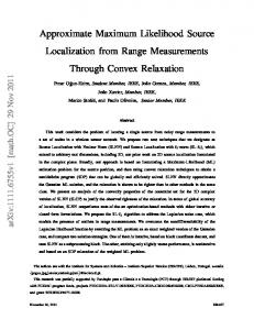
l(X; θ) = exp(−|A|)α(θ)−1 βn θs(X) where the normalizing constant is C(θ) = α(θ)/ exp(−|A|)n! The case θ = 1 corresponds to a Poisson process with intensity β. If θ = 0, the result is a simple inhibition process that contains no events at a distance less than or equal to r. Values of θ < 1 correspond to regularity of events, whilst for θ > 1 the process should result in clustering (see Figures 1a, 1b and 1c). For a clustered pattern, as was pointed out by Kelly and Ripley (1976), the condition θ > 1 violates the requirement of a finite normalizing constant C(θ) in (1). This problem can be removed by conditioning to the number of events, say N = n. This is not an artificial restriction because n(X) usually provides little information about the interactions among the events. The effect on conditioning to the MLE for the Strauss family has been demonstrated by Geyer and Moller (1994). Furthermore, conditioning on n makes it easier to generate simulations by the discretetime Markov chain method of Ripley (1979, 1987). The conditional likelihood function for the Strauss process is given by (2)

ln (X; θ) = θs(X) /Cn (θ)

where the normalizing constant is given by (3)

Cn (θ) =

Z

An

θs(X) dx1 · · · dxn .

Maximum likelihood estimation of θ requires the evaluation of (3) which is not usually obtainable in closed form. We therefore try to maximize an approximation to the likelihood function. In the following, we develop approximations to the MLE for the Strauss conditional model.

6

1.0

0.0 0.2 0.4 0.6 0.8 1.0 theta=1,s(X)=43

0.8 0.0

0.2

0.4

0.6

• • • • • •

•

1.0 0.8 0.6

••

• •

• 0.2

• •

• ••••• ••

1.0 0.8

• • • •••

• • • • • • • • •• • • ••• • • • • • • ••

0.0 0.2 0.4 0.6 0.8 1.0 theta=1.1,s(X)=62

0.6

• •

•

•

0.4

•

• •

0.2

•

• • • • •

•

• •

•

• • • •

• ••

• • • • •

• •

•

• ••

• •• •

• ••

•

0.0 0.2 0.4 0.6 0.8 1.0 theta=0.8,s(X)=23

0.0

• • • • •

•

0.4

• •

0.0

1.0 0.8 0.6 0.4 0.2

•

•

• •

•

•

•• • •• •

• •• • • • • • • • • • • • • •

• •• • • •• •

••• • • •• • •• • •• • • • • • • • • ••

•

• •

0.0 0.2 0.4 0.6 0.8 1.0 theta=1.2,s(X)=65

• •• •

•

• • • •

• •

• • •

•

• •

•

• •

• • ••• •• • • • • • •• • • •

• • •

•

•

1.0 0.8

•

•• • • • • • • • • • • • • • •• • • •• • • • •• • • • • •• • • • • • • • • •

• •

• • •

• •

•

• • •

•

•

•• •

•

• •

0.6

• •

0.4

•

0.2

•

•

••

•

0.0 0.2 0.4 0.6 0.8 1.0 theta=0.4,s(X)=19

0.0

1.0 0.8 0.6 0.4 0.2 0.0

•

•

• • • •• •

•

0.0 0.2 0.4 0.6 0.8 1.0 theta=0.1,s(X)=7

•

•

•• •

0.0

1.0 0.8 0.6 0.4 0.2 0.0

• • • • • • • • • • • • • • • • • • • • • • • • • • • • • • • • • • • • • • • • • • • • • • • • • •

• • ••

• ••

0.0 0.2 0.4 0.6 0.8 1.0 theta=1.3,s(X)=71

Figure 1a. Realizations of simulated patterns under the Strauss model for different values of Figure 1a. parameter θ. In each pattern it is also included s(X), the number of neighbour pairs. Figure 1a. r=0.10

7

•

•

1.0 0.8

• •

•

0.6

•

• •• •

0.4

•• • • • • • • • •

•

• •• •• •

1.0 0.8 0.6 0.4

• • • • •• • • • • •• •• •• • •• • •• • • • • • •• • • • • •

• •• • • •

•

••

•

• •

• •

•

• •• • • • • • • • •• • • • • • • • • • • • • • • •

0.0 0.2 0.4 0.6 0.8 1.0 theta=0.8,s(X)=56

• •

• • • • •

0.0 0.2 0.4 0.6 0.8 1.0 theta=1.1,s(X)=84

• • • •

••

•

• • • • • • • • •• • •

• • • • ••

•

• • • •

• • • • •• •• •

•• • • ••• • ••

0.0 0.2 0.4 0.6 0.8 1.0 theta=1.2,s(X)=127

•••••••••••••• • ••••••••• • ••••

0.0

0.2

0.4

0.6

0.8

1.0

0.0 0.2 0.4 0.6 0.8 1.0 theta=1,s(X)=74

• •

0.2

• • • • •• • • • • •• • • • • • • • •• • • • • • •• • • •• • • • • •• • • • • • • • •• • • •

• •

0.0 0.2 0.4 0.6 0.8 1.0 theta=0.4,s(X)=39

0.0

0.0

0.2

0.4

0.6

0.8

1.0

0.0 0.2 0.4 0.6 0.8 1.0 theta=0.1,s(X)=22

•

0.2

•

•

••

0.0

••

0.8

1.0

• ••

•

••

• •

•

1.0

• •

•

•

•• •

• • •

•

• • • •

0.8

• •

•

•

• •

0.6

•

•

•

•

•

•

0.4

••

0.6

•

•

•

•

••

0.2

•

•

••

•

0.0

• •

•

•

••

•

•• •

0.4

0.6 0.4

•

0.2 0.0

•

• •

•

0.2

•

• •

•

•

0.0

•

•

••

0.8

1.0

••

0.0 0.2 0.4 0.6 0.8 1.0 theta=1.3,s(X)=1205

Figure 1b. Realizations of simulated patterns under the Strauss model for different values of Figure 1a. parameter θ. In each pattern it is also included s(X), the number of neighbour pairs. Figure 1a. r=0.15

8

•

••

• ••

•

•

• •••• • • • •• • • • • • • •• • • • •• • • • • •

0.0 0.2 0.4 0.6 0.8 1.0 theta=1.1,s(X)=174

1.0 0.8

•

••

• • •

• •

•

• •• •

•

• •• • •

•

• ••

• •

••

•

•

•

0.0 0.2 0.4 0.6 0.8 1.0 theta=0.8,s(X)=89

1.0

1.0

•

•

•

•

•

• •

•

• •••• •••• • •• • ••• • • •••••••••••• • •• • •• • •

0.0 0.2 0.4 0.6 0.8 1.0 theta=1.2,s(X)=1127

• • • ••• ••• ••• •••••••• •••• • •• ••• ••••••• •

0.0

0.2

0.4

0.6

0.8

1.0

0.0 0.2 0.4 0.6 0.8 1.0 theta=1,s(X)=147

•

• •• • • • • • • • •• • • • • • •

0.8

• • • • • • • •• • • • • • • • • •• ••• • • • • •• • • • •• • • • • • • • • • • •

• • •

0.6

•

••

0.4

••

• •

0.2

•

••

0.0 0.2 0.4 0.6 0.8 1.0 theta=0.4,s(X)=72

0.0

0.0

0.2

0.4

0.6

0.8

1.0

0.0 0.2 0.4 0.6 0.8 1.0 theta=0.1,s(X)=43

•

•

•• • •

•

••

•

•

0.8

• ••

••

•

• •

•

•• •

0.6

•

••

•

•

0.4

••

••

0.2

0.2

••

• •

•

0.2

••

•

• • • • •

• ••

• ••

•

0.0

• • •

• •

•

0.6

0.6

•• •

•

•

•

0.4

••

•

•

0.2

0.8

• • •

•• • •

•

0.0

1.0

• •

•

0.4

•

••

0.0

•

•

0.0

1.0 0.8

•

•

• ••

0.4

0.6

•• • •

0.0 0.2 0.4 0.6 0.8 1.0 theta=1.3,s(X)=1194

Figure 1c. Realizations of simulated patterns under the Strauss model for different values of Figure 1a. parameter θ. In each pattern it is also included s(X), the number of neighbour pairs. Figure 1a. r=0.20

9

2.1. Method of Ogata-Tanemura Ogata and Tanemura (1981) proposed to use a cluster-expansion method of statistical mechanics assuming that the events of the point process are sparsely distributed, so that third and higher-order cluster integrals are negligible. Then, using up to the secondorder cluster integral, an approximation to the normalizing constant is given by ½ ¾ b(θ) n(n−1)/2 Cn (θ) = |A| 1 − |A| n

where b(θ) is, for the Strauss model, b(θ) = π(1 − θ)r2 . Then, the MLE is given by © ª 2 s(X) 2|A| − πr b (4) θ= 2 . πr (n(n − 1)/2 − s(X)) 2.2. Method of Penttinen Penttinen (1984) proposed another sparse-data approximation to (3), which for the Strauss model takes the form © ª Cn (θ) = exp 1/2n(n − 1)πr2 (θ − 1)

and the MLE is given by (5)

b θ=

s(X) . 1/2n(n − 1)πr2

2.3. Method of virial expansions This method consists of the following approximation of (3), (6) R R n−1 log(Cn ) ≈ (bn /2) ℜ2 f12 dx2 + (b2n /4) ℜ4 f12 f13 f23 dx2 dx3 + R (b3n /8) ℜ6 ( f12 f13 f14 f23 f24 f34 + 6 f12 f13 f14 f23 f24 + 3 f12 f14 f23 f34 )dx2 dx3 dx4 + · · · ° ° where bn = n/|A| and fi j = exp(−Φ(°xi − x j ° ; θ)) − 1 (Ripley, 1988). To implement this method for the Strauss process we use the fourth order expansion obtained by calculating the integrals in (6): n! log(Cn (θ)) = −πn(n − 1)Ψr2 /(2|A|) − 0,29325π2 (n−3)! Ψ3 r4 /(6|A|2 ) n! 6 5 4 3 −π (n−4)! {−0,27432Ψ + 2,18542Ψ − 1,37886Ψ }r6 /(24|A|3 )

10

where Ψ = 1 − θ. Then solving (7)

d log(Cn (θ))/dθ = s(X)/θ

we obtain b θ, the approximate MLE of θ.

2.4. Stochastic approximation based on a Newton-Raphson procedure Penttinen (1984) suggested a Newton-Raphson type algorithm for solving the maximum likelihood estimating equation. Assume Φ(t; θ) is twice differentiable with respect to θ. Differentiation of both sides of equation (3) yields −∂Cn (θ) = Cn (θ)Eθ [∂Un (x1 , . . . , xn ; θ)/∂θ] ∂θ where the total potential energy, for the Strauss process, is Un (x1 , . . . , xn ; θ) = − log θs(X) . The MLE b θ solves ∂ log(ln (X; θ))/∂θ = 0. If b θ0 denotes an initial guess for b θ, then the Newton-Raphson algorithm consists of

where (8) and

h i−1 b θk+1 = b θk − ΓT (b θk ) βT (b θk ) k = 0, 1, 2, . . . 1 βT (b θk ) = T

T

1

∑ bθ

t=1

[s(X) − s(φn (t))]

k

1 T ΓT (b θk ) = T1 ∑t=1 [s(φn (t)) − s(X)] b θ2k o2 n θk ) . − b1 [s(X) − s(φn (t))] − βT (b θk

Note that φn (1), . . . , φn (T ) are simulated according to a Strauss process with parameter b θk . 2.5. Stochastic approximation based on Robbins-Monro procedure

This stochastic approximation procedure was first introduced by Robbins and Monro (1951) and can be used to estimate the solution θ∗ of an equation F(θ∗ ) = ϕ when 11

there is very little information about the function F but it is possible, for any given θ, to generate a random variable Tθ with expectation E(Tθ ) = F(θ). For the Strauss model, the goal is to solve M(b θ) = s(X)

(9)

for b θ, where X is the observed data and M(θ) = Eθ [s(X)]. Then we set Tθ = s(Xθ ), where Xθ is a simulated Strauss process with parameter θ and we obtain, recursively, a sequence of estimates of b θ using ª B© s(X) − s(Xθk ) . k

θk+1 = θk +

Then θk → b θ (a.s.) (Moyeed and Baddeley, 1991).

Defining µ = M ′ (b θ) and σ2 = Varθ [s(X)], if B > 1/(2µ) then θk is asymptotically normally distributed with mean b θ and variance B2 σ2 /(2Bµ − 1).

The starting value θ0 is arbitrary, but should be set to an initial approximation such as that holding in the sparse case θ0 =

2s(X)|A| . n(n − 1)πr2

The optimum B, Bopt , could be estimated by Bopt = or Bopt =

1 1 = µ M ′ (b θ) 2|A| . n(n − 1)πr2

3. A SIMULATION STUDY 3.1. Edge-correction Commonly, the region A is a sampled sub-region of a much larger region within which the phenomenon operates and some form of edge-correction is vital. When A is a rectangle, a possible strategy is to map A onto a torus by identifying opposite edges. This periodic boundary is commonly used for computer experiments in statistical mechanics. 12

However, for the analysis of real data, periodic boundaries can introduce undesirable artefacts: toroidal distances can be arbitrarily small even when the underlying process has a positive hard-core distance. In the present comparative simulation study, the points patterns were themselves generated using a periodic boundary, then this particular difficulty does not arise. To compensate for the omission of contributions to the total potential from unobserved events outside A we replace summations of the form ° ° ∑ Φ(°xi − x j ° ; θ) j>i

by

° ° 1 ° ° w−1 ∑ i j Φ( xi − x j ; θ) 2 j6=i

where w°i j is the proportion of the circumference of the circle with centre xi and radius ° °xi − x j ° which is contained within A. This is an adapted version of Ripley’s correction (Ripley, 1977, 1988). The majority of available edge-corrections correct the bias using lengths or areas of parts of circles or discs, respectively. In the simulation study, we also include results using the so-called free boundary conditions, in which no edge-correction at all is made. 3.2. Standard Errors One possible way to obtain approximate standard errors is by using Monte Carlo methodology. For this approach, we simulate s realisations with θ = b θ, the point estimate under the chosen method for the original data. We then evaluate point estimates b θ j , j = 1, . . . , s from the simulated patterns and use the empirical distribution of the b θ j as an approximation to the sampling distribution of b θ. In particular, the sample mean and standard deviation of the b θ j give useful indications of the bias and efficiency of estimation. This Monte Carlo approach is highly computer-intensive and it is usually known as parametric bootstrap. 3.3. Simulation method The spatial birth-and-death process provides the framework under which Ripley (1977, 1979) proposes to simulate a Markov point process on the bounded Borel set A ⊂ ℜd with n fixed. The method is related to Markov processes used in statistical mechanics and surveyed by Hastings (1970). Consider a set of particles interacting according to a certain potential function on a set A with periodic boundary, i.e. A is identified 13

with a torus. First, select n events from a uniform distribution on A; call this initial point pattern φn (0). At step (t + 1), delete systematically in turn one of the n events of φn (t) = {x1 , . . . , xn }, say event xi , and let φn (t) − {xi } denote the point pattern formed by removing xi from φn (t). Let p(u; φn (t) − {xi }) =

ln (φn (t) − {xi }, u) ln−1 (φn (t) − {xi })

denote the conditional intensity at u ∈ A given φn (t) − {xi }. Define M = sup p(u; φn (t) − {xi }). u∈A

Select an event u from a uniform distribution on A and set φn (t + 1) = {φn (t) − {xi }, u} with probability p(u; φn (t)−{xi })/M; otherwise, selection is repeated until a qualifying u is found. This method ensures that samples taken every n steps have no points in common. Ultimately, convergence to a Markov point process with likelihood ln (.) will occur. Unfortunately, in the case of the Strauss model, for θ much larger than 1 the algorithm is very slow and may result in simulation difficulties (see Figures 1b and 1c when θ = 1,2 and 1,3). 3.4. Design of the Simulation Study For the simulation study we selected eight parameter values: θ = 0,1, 0,4 and 0,8 corresponding to regular patterns; θ = 1 for the random pattern (Poisson process) and θ = 1,1, 1,2 and 1,3 for clustered ones (strongly interactive patterns). We also considered three different ranges of interaction: r = 0,1, 0,15 and 0,2. For each combination of parameter value and range of interaction we simulated 100 realizations, each one with n = 50 events on A the unit square. From the simulated realization we evaluated the estimate of θ using the five methods of approximation described in Section 2 and incorporating the edge-correction described in Section 3.1. Each combination of parameter value, interaction range, method of estimation and edge-correction (no edge-correction, Ripley’s and toroidal (periodic)) therefore yielded 100 estimates b θ j , j = 1, . . . , 100, which are summarised by the box-plots shown in Figures 2a, 2b and 2c.

14

1.0 0.8

0.8

0.0

-0.2 0.0

0.2

0.2

0.4

0.4

0.6

0.6

0.4 0.2 0.0 -0.2 -0.4

theta=0.8 1.2

theta=0.4 1.0

0.6

theta=0.1

OTf ri t Pf ri t VEf ri t NRf ri t RMf ri t

OTf ri t Pf ri t VEf ri t NRf ri t RMf ri t

theta=1

theta=1.1

theta=1.2

0.5 0.0

0.4

0.5

0.6

0.8

1.0

1.0

1.0

1.5

1.2

1.5

1.4

OTf ri t Pf ri t VEf ri t NRf ri t RMf ri t

OTf ri t Pf ri t VEf ri t NRf ri t RMf ri t

OTf ri t Pf ri t VEf ri t NRf ri t RMf ri t

OTf ri t Pf ri t VEf ri t NRf ri t RMf ri t

-0.5

0.0

0.5

1.0

1.5

2.0

2.5

theta=1.3

OTf ri t Pf ri t VEf ri t NRf ri t RMf ri t

Figure 2a. Box-plots of simulated parameter estimates. The horizontal lines indicate the true value of θ. The upper case letter identifies the method of estimation (OT=Ogata-Tanemura, P=Penttinen, VE=Virial Expansions, NR=Newton-Raphson, RM=Robbins-Monro), the lower case letter identifies the boundary condition (f=free, ri=Ripley, t=toroidal). r=0.10

15

theta=0.8 1.2

theta=0.4

0.8 0.4

-0.5

0.0

0.2

0.0

-0.4 -0.2 0.0

0.2

0.6

0.5

0.4

0.6

1.0

1.0

0.8

theta=0.1

OTf ri t Pf ri t VEf ri t NRf ri t RMf ri t

OTf ri t Pf ri t VEf ri t NRf ri t RMf ri t

theta=1

theta=1.1

theta=1.2

OTf ri t Pf ri t VEf ri t NRf ri t RMf ri t

2.0 1.5 1.0 0.5 0.0

0.4

0.6

0.8

1.0

1.2

0.4 0.6 0.8 1.0 1.2 1.4 1.6 1.8

OTf ri t Pf ri t VEf ri t NRf ri t RMf ri t

OTf ri t Pf ri t VEf ri t NRf ri t RMf ri t

OTf ri t Pf ri t VEf ri t NRf ri t RMf ri t

0.5

1.0

1.5

2.0

2.5

theta=1.3

OTf ri t Pf ri t VEf ri t NRf ri t RMf ri t

Figure 2b. Box-plots of simulated parameter estimates. See legend of Figure 2a. r=0.15

16

0.0 0.2 0.4

0.6 0.4 0.2 0.0 -0.4 -0.2

theta=0.8 0.6 0.8 1.0 1.2

theta=0.4 -0.2 0.0 0.2 0.4 0.6 0.8 1.0

0.8

theta=0.1

OTf ri t Pf ri t VEf ri t NRf ri t RMf ri t

OTf ri t Pf ri t VEf ri t NRf ri t RMf ri t

theta=1

theta=1.1

theta=1.2

OTf ri t Pf ri t VEf ri t NRf ri t RMf ri t

1.5 1.0 0.5 0.0

0.4

0.4

0.6

0.6

0.8

0.8

1.0

1.0

1.2

1.2

1.4

1.4

OTf ri t Pf ri t VEf ri t NRf ri t RMf ri t

OTf ri t Pf ri t VEf ri t NRf ri t RMf ri t

OTf ri t Pf ri t VEf ri t NRf ri t RMf ri t

-1

0

1

2

3

4

theta=1.3

OTf ri t Pf ri t VEf ri t NRf ri t RMf ri t

Figure 2c. Box-plots of simulated parameter estimates. See legend of Figure 2a. r=0.20

17

Table 1. Sample means and standard errors of parameter estimates when the interaction radius is r = 0,10. Each entry is based on 100 replicate Table 1. simulations of n=50 events on the unit square. Lower case letters indicate the boundary condition: free, Ri=Ripley and toro=toroidal.

r=0.10

O-T method free

Ri

toro

Pent. method free

Ri

toro

θ

V-E method free

Ri

N-R method toro

R-M method

free

Ri

toro

free

Ri

toro

Sample Means

18

0.1

0.247

0.231

0.091

0.193

0.176

0.087

0.112

0.125

0.122

0.095

0.097

0.098

0.093

0.091

0.096

0.4

0.434

0.427

0.407

0.541

0.308

0.345

0.456

0.319

0.376

0.305

0.403

0.393

0.231

0.378

0.404

0.8

0.645

0.714

0.835

0.703

0.715

0.732

0.913

0.809

0.805

0.704

0.791

0.807

0.710

0.803

0.824

1.0

0.831

0.873

1.041

0.810

0.912

1.013

0.919

0.920

0.946

0.910

0.935

0.931

0.847

1.079

0.979

1.1

0.914

0.979

1.093

0.973

1.007

1.081

1.013

1.315

1.291

1.004

1.073

0.993

1.215

1.183

1.032

1.2

0.997

1.101

1.103

1.031

1.046

1.097

1.035

1.416

1.335

1.053

1.143

1.103

1.392

1.194

1.197

1.3

1.124

1.445

1.213

1.093

1.106

1.148

1.056

1.496

1.531

1.197

1.292

1.197

1.431

1.393

1.245

θ

Standard Errors

0.1

0.215

0.210

0.091

0.141

0.115

0.091

0.090

0.091

0.037

0.093

0.051

0.047

0.061

0.057

0.053

0.4

0.171

0.135

0.131

0.205

0.217

0.215

0.099

0.101

0.048

0.039

0.032

0.031

0.043

0.038

0.029

0.8

0.176

0.156

0.132

0.115

0.043

0.039

0.105

0.101

0.066

0.127

0.125

0.112

0.128

0.118

0.105

1.0

0.125

0.112

0.111

0.127

0.115

0.113

0.107

0.096

0.080

0.098

0.083

0.081

0.103

0.097

0.065

1.1

0.215

0.203

0.193

0.235

0.215

0.195

0.135

0.137

0.122

0.121

0.115

0.107

0.120

0.119

0.117

1.2

0.323

0.213

0.211

0.341

0.312

0.247

0.156

0.165

0.146

0.143

0.135

0.127

0.142

0.138

0.129

1.3

0.351

0.225

0.212

0.451

0.410

0.393

0.170

0.171

0.157

0.161

0.149

0.143

0.160

0.153

0.141

Table 2. Sample means and standard errors of parameter estimates when the interaction radius is r = 0,15.

r=0.15

O-T method free

Ri

toro

Pent. method free

Ri

toro

θ

V-E method free

Ri

N-R method toro

R-M method

free

Ri

toro

free

Ri

toro

Sample Means

19

0.1

0.197

0.215

0.142

0.198

0.186

0.082

0.197

0.183

0.172

0.094

0.096

0.096

0.092

0.092

0.093

0.4

0.431

0.416

0.412

0.515

0.412

0.319

0.511

0.392

0.431

0.304

0.393

0.409

0.214

0.341

0.431

0.8

0.613

0.705

0.841

0.609

0.674

0.705

0.819

0.812

0.811

0.703

0.793

0.805

0.695

0.849

0.907

1.0

0.813

0.912

1.010

0.805

0.845

0.906

0.905

0.896

0.915

0.921

0.935

0.963

0.896

0.945

1.031

1.1

0.887

0.946

1.035

0.874

0.885

0.948

1.193

1.203

1.195

0.973

0.987

0.995

0.994

0.998

1.051

1.2

0.944

0.997

1.102

1.005

1.045

1.103

1.298

1.305

1.399

1.047

1.031

1.034

1.314

1.293

1.227

1.3

1.034

1.125

1.204

1.091

1.112

1.131

1.423

1.397

1.430

1.092

1.141

1.195

1.443

1.348

1.338

θ

Standard Errors

0.1

0.212

0.205

0.146

0.150

0.141

0.115

0.102

0.052

0.036

0.091

0.050

0.045

0.061

0.060

0.055

0.4

0.202

0.165

0.108

0.210

0.231

0.212

0.103

0.096

0.047

0.039

0.037

0.031

0.048

0.035

0.028

0.8

0.176

0.135

0.126

0.212

0.195

0.118

0.105

0.037

0.071

0.131

0.129

0.125

0.127

0.121

0.113

1.0

0.146

0.131

0.127

0.210

0.196

0.121

0.104

0.096

0.091

0.103

0.095

0.091

0.113

0.093

0.091

1.1

0.215

0.201

0.153

0.235

0.221

0.198

0.135

0.131

0.118

0.125

0.121

0.119

0.125

0.122

0.119

1.2

0.345

0.303

0.246

0.319

0.312

0.251

0.158

0.162

0.135

0.148

0.137

0.132

0.157

0.138

0.118

1.3

0.431

0.397

0.353

0.425

0.418

0.401

0.177

0.182

0.152

0.159

0.152

0.151

0.191

0.153

0.139

Table 3. Sample means and standard errors of parameter estimates when the interaction radius is r = 0,20.

r=0.20

O-T method free

Ri

toro

Pent. method free

Ri

toro

θ

V-E method free

Ri

N-R method toro

R-M method

free

Ri

toro

free

Ri

toro

Sample Means

20

0.1

0.240

0.273

0.184

0.210

0.221

0.082

0.253

0.231

0.165

0.092

0.093

0.093

0.090

0.091

0.093

0.4

0.450

0.443

0.415

0.539

0.495

0.324

0.551

0.453

0.397

0.241

0.295

0.335

0.221

0.298

0.321

0.8

0.595

0.593

0.625

0.605

0.614

0.693

0.719

0.771

0.789

0.615

0.693

0.705

0.630

0.710

0.747

1.0

0.841

0.855

0.931

0.741

0.793

0.845

0.810

0.839

0.921

0.710

0.845

0.947

0.708

0.793

0.810

1.1

0.872

0.879

0.947

0.793

0.815

0.897

0.915

0.986

1.023

0.941

0.943

0.998

0.983

0.995

1.108

1.2

0.936

0.979

0.998

0.847

0.895

0.913

1.005

1.039

1.103

1.009

1.015

1.074

1.334

1.321

1.253

1.3

1.013

1.115

1.197

0.915

0.945

1.041

1.027

1.093

1.154

1.051

1.123

1.147

1.451

1.382

1.324

θ

Standard Errors

0.1

0.230

0.211

0.135

0.151

0.134

0.127

0.105

0.104

0.098

0.091

0.085

0.073

0.065

0.058

0.047

0.4

0.215

0.197

0.109

0.198

0.197

0.201

0.107

0.107

0.098

0.102

0.098

0.085

0.058

0.032

0.019

0.8

0.178

0.167

0.132

0.201

0.195

0.119

0.103

0.102

0.101

0.131

0.130

0.121

0.115

0.103

0.102

1.0

0.153

0.136

0.131

0.203

0.201

0.202

0.104

0.095

0.092

0.134

0.128

0.112

0.121

0.098

0.095

1.1

0.198

0.185

0.176

0.218

0.212

0.205

0.142

0.139

0.126

0.141

0.139

0.129

0.128

0.125

0.123

1.2

0.351

0.298

0.255

0.325

0.301

0.247

0.181

0.173

0.148

0.158

0.138

0.132

0.199

0.143

0.128

1.3

0.398

0.299

0.301

0.441

0.412

0.395

0.183

0.179

0.165

0.171

0.163

0.159

0.183

0.161

0.146

3.5. Results and discussion Tables 1, 2 and 3 give the results of the simulation study, expressed in terms of the sample means, θ and standard errors, sθ . These two statistics characterize the sampling distribution of the parameter estimates as noted in section 3.2 above as neither the theoretical nor asymptotic approximations of the parameter distribution are not known. The bias and efficiency of the estimation can only be assessed by means of a Monte Carlo approach. However, Bayesian procedures could also be used to approach the theoretical parameter distribution as in Mateu and Montes (1995). The table values indicate that both stochastic approximation methods, Newton-Raphson (N-R) and Robbins-Monro (R-M), exhibited better results, in terms of bias and standard errors, than Ogata-Tanemura (O-T) and Penttinen (P) methods for cases of strong regularity (θ ≤ 0,4) and clustering (θ ≥ 1,1). The approximate maximum likelihood method based on virial expansions (V-E) exhibited substantial bias, particularly when θ is large; however, this is qualitatively predictable on theoretical grounds, since the adequacy of the approximation to the likelihood deteriorates as θ increases. Implementation of this approximation for any potential is straightforward if only low-order virial coefficients are required. This method is not suited for estimation in cases of strong interaction. The O-T and P approximate maximum likelihood methods provided substantial negative bias for medium-to-large values of θ giving relatively large standard deviations for these values. These two approximations are based on the sparseness assumption and are not reliable methods for clustered patterns for which higher-order interactions become important. Inspecting the standard errors in conjunction with the range of θ, we observe that approximate maximum likelihood using O-T and P methods, provide large standard deviations for small (θ ≤ 0,4) and large (θ ≥ 1,1) values of parameter θ and, in any case, they are much larger than those obtained with the other three methods. For different values of θ, the choice of boundary condition becomes important. Generally, for any method and parameter values, the periodic boundary condition produced better results than Ripley’s, and in turn they are better than those obtained with the free boundary condition. The N-R and R-M approximate maximum likelihood methods provided unbiased and efficient estimates for all ranges of parameter values, under periodic and Ripley’s boundary condition. However, they provided biased estimates under the free boundary condition. Comparing the behaviour of the bias and the standard errors of estimates among the three interaction radii, we observe that, under the same parameter value, method of estimation and boundary condition, biases and standard errors increased with r providing worse estimates for r = 0,2 compared with r = 0,1. For example, for r = 0,2 and using the R-M procedure with Ripley’s correction, we get significant bias compared with the 21

unbiased and efficient estimates obtained under the same conditions but with r = 0,1. Apart from this, all properties analysed above are also true for different interaction radii. The Strauss process with θ > 1 is not a good model for applications. It may result in simulation difficulties such as sensitivity to edge-conditions, poor mixing, etc (Gates and Westcott, 1986). Moreover, the spatial birth-and-death approach might not be the optimal choice. For the well-defined case θ < 1, exact simulation of the Strauss process is possible using the Propp-Wilson algorithm (Moller, 1998; Kendall and Moller, 1999). Concerning edge-corrections, another possibility is to apply conditional simulation: simulate a point pattern into some guard area using the model conditional on the observed point pattern and then apply the guard area events in estimation.

4. CONCLUSIONS The conclusions, taking into account the results of our simulation study, are the following: 1. Stochastic approximations generally provide better results, particularly for mediumto-large parameter values, than those based on the sparseness assumption which are not suited for estimation in cases of strong interaction. For small parameter values and small interaction radius (r = 0,1), the Ogata-Tanemura approximation exhibits very good results. 2. For small interaction radius and using stochastic approximations, Ripley’s and periodic boundary condition provide unbiased and efficient estimates. This is not true when r increases. 3. Generally, periodic and Ripley’s boundary condition exhibit better results than free boundary condition. 4. When r increases the biases and the standard errors increase for any method, particularly for the approximate maximum likelihood methods. 5. Finally, in cases of clustered processes we recommend to use stochastic approximations with Ripley’s or toroidal boundary condition. In cases of strong regularity, we could also use approximations based on the sparseness assumption.

22

ACKNOWLEDGEMENTS The referees are gratefully acknowledged for their helpful comments that have substantially improved an earlier version of the paper.

REFERENCES Baddeley, A. and Moller, J. (1989). «Nearest-neighbour Markov point processes and random sets». International Statistical Review, 57, 89-121. Baddeley, A. and van Lieshout, M.N.M. (1993). «Stochastic geometry in high-level vision». In Statistics and images, K.V. Mardia and G.K. Kanji (Eds.), Vol. 1 of Advances in Applied Statistics, 231-256. Besag, J.E. (1974). «Spatial interaction and the statistical analysis of lattice systems (with discussion)». Journal of the Royal Statistical Society B, 36, 192-236. Cressie, N. (1993). Statistics for Spatial Data. New York: John Wiley and Sons, Revised edition. Daley, D.J. and Vere-Jones, D. (1988). Introduction to the theory of point processes. New York: Springer. Diggle, P.J. (1983). Statistical Analysis of Spatial Point Patterns. London: Academic press. Diggle, P.J., Fiksel, T., Grabarnik, P, Ogata, Y., Stoyan, D. and Tanemura, M. (1994). «On parameter estimation for pairwise interaction point processes». International Statistical Review, 62, 99-117. Diggle, P.J., Gates, D.J. and Stibbard, A. (1987). «A nonparametric estimator for pairwise interaction point processes». Biometrika, 74, 763-70. Gates, D.J. and Westcott, M. (1986). «Clustering estimates for spatial point distributions with unstable potentials». Annals of the Institute of Statistical Mathematics, 38, 123-135. Geman, S. and Geman, D. (1984). «Stochastic relaxation, Gibbs distributions and the Bayesian restoration of images». IEEE Transactions on Pattern Analysis and Machine Intelligence, 6, 721-741. Geyer, C.J. and Moller, J. (1994). «Simulation and likelihood inference for spatial point processes». Scandinavian Journal of Statistics, 21, 359-373. Geyer, C.J. and Thompson, E.A. (1992). «Constrained Monte Carlo maximum likelihood for dependent data, (with discussion)». Journal of the Royal Statistical Society B, 54, 657-699.

23

Hastings, W.K. (1970). «Monte Carlo sampling methods using Markov chains and their applications». Biometrika, 57, 97-109. Kelly, F.P. and Ripley, B.D. (1976). «On Strauss’ model for clustering». Biometrika, 63, 357-60. Kendall, W.S. and Moller, J. (1999). «Perfect Metropolis-Hastings simulation of locally stable point processes». Manuscript. van Lieshout, M.N.M. and Baddeley, A. (1995). «Markov chain Monte Carlo methods for clustering of image features». In Proceedings of the fifth international conference on image processing and its applications, Vol. 410 of IEE Conference Publication, 241-245, London. Mateu, J. and Montes, F. (1995). «Inferencia Bayesiana en procesos puntuales Markov». In Proceedings of the V Spanish Conference of Biometry, 65-68, Valencia. Molina, R. and Ripley, B.D. (1989). «Using spatial models as priors in astronomical image analysis». Journal of Applied Statistics, 16, 193-206. Moller, J. (1998). «Markov chain Monte Carlo and spatial point processes». In Proceedings Seminaire Europeen de Statistique, “Stochastic geometry, likelihood and computation”. Barndorff-Nielsen, Kendall and Van Lieshout (eds), Chapman and Hall. Moyeed, R.A. and Baddeley, A. (1991). «Stochastic approximation of the MLE for a spatial point pattern». Scandinavian Journal of Statistics, 18, 39-50. Ogata, Y. and Tanemura, M. (1981). «Estimation of interaction potentials of spatial point patterns through the maximum likelihood procedure». Annals of the Institute of Statistical Mathematics, 33 B, 315-38. Penttinen, A. (1984). «Modelling interaction in spatial point patterns: parameter estimation by the maximum likelihood method». Jyvaskyla Studies in Computer Science, Economics and Statistics, 7. Ripley, B.D. (1977). «Modelling spatial patterns (with Discussion)». Journal of Royal Statistical Society B, 39, 172-212. Ripley, B.D. (1979). «Simulating spatial patterns: dependent samples from a multivariate density». Applied Statistics, 28, 109-12. Ripley, B.D. (1981). Spatial Statistics. New York: Wiley. Ripley, B.D. (1987). Stochastic Simulation. New York: Wiley. Ripley, B.D. (1988). Statistical Inference for Spatial Processes. Cambridge: Cambridge University press. Ripley, B.D. (1989). «Gibbsian interaction models». In Spatial Statistics: past, present and future (ed. D.A. Griffiths), New York: Image. Ripley, B.D. and Kelly, F.P. (1977). «Markov point processes». Journal of the London Mathematical Society, 15, 188-192. 24

Robbins, H. and Monro, S. (1951). «A stochastic approximation method». Annals of Mathematical Statistics, 22, 400-407. Stoyan, D., Kendall, W.S. and Mecke, J. (1995). Stochastic Geometry and its Applications. Berlin: Akademie-Verlag, 2nd Edition. Strauss, D.J. (1975). «A model for clustering». Biometrika, 62, 467-75. Strauss, D.J. (1986). «On a general class of models for interaction». SIAM Review, 28, 513-527. Takacs, R. (1986). «Estimator for the pair-potential of a Gibbsian point process». Math. Operationsf. Statist. Ser. Statist., 17, 429-33.

25