Approximate Relational Reasoning by Stochastic Propositionalization

Approximate Relational Reasoning by Stochastic Propositionalization Nicola Di Mauro, Teresa M.A. Basile, Stefano Ferilli, and Floriana Esposito

Abstract. For many real-world applications it is important to choose the right representation language. While the setting of First Order Logic (FOL) is the most suitable one to model the multi-relational data of real and complex domains, on the other hand it puts the question of the computational complexity of the knowledge induction process. A way of tackling the complexity of such real domains, in which a lot of relationships are required to model the objects involved, is to use a method that reformulates a multi-relational learning task into an attribute-value one. In this chapter we present an approximate reasoning method able to keep low the complexity of a relational problem by using a stochastic inference procedure. The complexity of the relational language is decreased by means of a propositionalization technique, while the NP-completeness of the deduction is tackled using an approximate query evaluation. The proposed approximate reasoning technique has been used to solve the problem of relational rule induction as well as the task of relational clustering. An anytime algorithm has been used for the induction, implemented by a population based method, able to efficiently extract knowledge from relational data, while the clustering task, both unsupervised and supervised, has been solved using a Partition Around Medoid (PAM) clustering algorithm. The validity of the proposed techniques has been proved making an empirical evaluation on real-world datasets.

1 Motivations Most of the acquired large volumes of data in digital format are stored using relational databases consisting of multiple tables and relations. Moreover, the data used in the fields of user behaviour modelling, protein fold recognition Nicola Di Mauro · Teresa M.A. Basile · Stefano Ferilli · Floriana Esposito Department Of Computer Science, University of Bari, Italy e-mail: {ndm,basile,ferilli,esposito}@di.uniba.it Z.W. Ras and L.-S. Tsay (Eds.): Advances in Intelligent Information Systems, SCI 265, pp. 81–109. c Springer-Verlag Berlin Heidelberg 2010 springerlink.com 

82

N. Di Mauro et al.

and drug design are relational in nature, and the induction of conceptual definitions modelling the knowledge of such complex real-world domains is a hard and crucial task. The challenges posed by such domains are due to various factors such as the noise in the object descriptions, the lack of data, but also the choice of the representation language exploited to describe them. The choice of the right representation language is a fundamental as well as a critical aspect in the process of knowledge discovery. Indeed, the used representation language has a significant impact on the performance of the learning algorithms but also on the possibility to interpret and reuse the discovered knowledge. The most suitable representation language to describe the objects and their relationships of complex real-world domains is a logicbased representation such as the first-order logic language (FOL), a natural extension of the propositional representation. Inductive Logic Programming (ILP) [23] systems are able to learn hypotheses expressed with this more powerful language. ILP systems represent examples, background knowledge, hypotheses and target concepts in Horn clause logic. The core of ILP is the use of logic for representation and the search for syntactically legal hypotheses constructed from predicates provided by the background knowledge. However, this representation language allows a potentially great number of mappings between descriptions (relational learning), differently from the feature vector representation in which only one mapping is possible between descriptions (propositional learning). The obvious consequence of such a representation is that both the space of candidate solutions to search and the test to assess the validity of the induced model are more costly. A possible solution is represented by approximate reasoning techniques [32], that try to decrease the complexity of a problem changing either the adopted language or the inference operation used for the deduction. In this way, the results may be unsound or incomplete but with a consequent speed-up and a reduced reasoning complexity. A possible approximate reasoning technique consists in reformulating the original multi-relational learning task in a propositional one (i.e., propositionalization). This reformulation can be partial (heuristic), in which information is lost and the representation change is incomplete, or complete, in which no information is lost. In general, however, it is not possible to efficiently transform multi-relational data into an equivalent propositional form without an exponentially increasing complexity [26]. Alternative approaches concern the possibility to apply propositionalization directly on the original FOL context by a sort of flattening of the multi-relational data substituting them with all (or a subset of) their matchings with a pattern that can be provided by the users or previously built by the system. This work presents a stochastic propositionalization technique for relational descriptions, introduced in [9, 10] for building efficient induction algorithms, and here extended and applied for approximate relational clustering. In particular, we propose a method useful to decrease the dimensionality of the space of candidate solutions of a multi-relational learning problem

Approximate Relational Reasoning by Stochastic Propositionalization

83

to search by means of a propositionalization technique in which the transposition of the relational data is performed by an online flattening of the examples. The proposed inductive method is a population based (genetic) algorithm that stochastically propositionalizes the training examples in which the learning phase may be viewed as a bottom-up search in the hypotheses space. While, the proposed clustering method is an extension of the Partition Around Medoid (PAM) [16] algorithm to the relational case, where the same propositionalization technique has been used to define a distance measure between relational descriptions. The objective of this chapter is threefold: O1: providing an efficient and scalable technique for relational inductive reasoning, combining a genetic approach to navigate the search space of candidate solutions with a partial transposition of the relational knowledge base in a propositional one; O2: adopting an approximate reasoning strategy in a relational inductive learner, making incomplete a) the validation test (query answering) of the acquired model, and b) the inductive generalization task; O3: using an approximate matching procedure of relational descriptions for computing a distance measure useful for conceptual clustering. The resulting learning algorithm, of the objective O1, belongs to the class of anytime algorithms [6] whose quality of results improves gradually as computation time increases, hence trading this quality against the cost of computation. They are resource constrained algorithms that return the best solution within a specified computational budget. The validation test of the acquired knowledge, in objective O2, corresponds to the classical query answering task, that in relational learning is obtained by solving a subsumption problem known to be NP-complete. In many cases it is less important to obtain an exact query result than keeping query response time short. For instance, the following conjunctive FOL query ← author(A1, P 1), journal(P 1, J), impact(J, IF ), author(A2, P 2), journal(P 2, J) may be used to test if there exist two authors A1 and A2 that have published a paper (resp. P 1 and P 2) in a journal J with an impact factor IF . Sometimes, instead of a correct answer, it may be suitable knowing the response for a subset of the authors in the domain, improving running time to the detriment of the accuracy. The approximate query answering used in this work is a sampling based technique, in which a random sample of the individuals involved in the domain is selected and used to solve the query. Results obtained for the approximate query answering technique, in the objective O3, have been extended for defining an approximate dissimilarity function between relational descriptions.

84

N. Di Mauro et al.

2 Stochastic Propositionalization In this section we present a technique [10, 9] that, reformulating the relational descriptions can be used to solve a multi-relational learning problem (both supervised and unsupervised).

2.1 Logic Background We used Datalog [31] as representation language for the domain and induced knowledge, that here is briefly reviewed. For a more comprehensive introduction to logic programming and ILP we refer the reader to [8, 19, 23]. Definition 1 (Alphabet). A first-order alphabet consists of a set, X , of variables, a set, L, of constants, a set, F , of function symbols, and a set, P = ∅, of predicate symbols. Each function symbol and each predicate symbol has a natural number (its arity) assigned to it. The arity of a function symbol represents the number of arguments the function has. Constants may be viewed as function symbols of arity 0. Definition 2 (Terms). A term is a constant symbol, a variable symbols, or an n-ary function symbol f ∈ F applied to n terms t1 , t2 , . . . , tn . An atom p(t1 , . . . , tn ) (or atomic formula) is a predicate symbol p ∈ P of arity n applied to n terms ti . Both l and its negation l are said to be literals (resp. positive and negative literal) whenever l is an atomic formula. Definition 3 (Clause). A clause is a formula of the form ∀X1 ∀X2 . . . ∀Xn (L1 ∨L2 ∨. . .∨Li ∨Li+1 ∨. . .∨Lm ) where each Li is a literal and X1 , X2 , . . . Xn are all the variables occurring in L1 ∨ L2 ∨ . . . Li ∨ . . . Lm . Most commonly the same clause is written as an implication L1 , L2 , . . . Li−1 ← Li , Li+1 , . . . Lm , where L1 , L2 , . . . Li−1 is the head of the clause and Li , Li+1 , . . . Lm is the body of the clause. Clauses, literals and terms are said to be ground whenever they do not contain variables. A Horn clause is a clause which contains at most one positive literal. A Datalog clause is a clause with no function symbols of non-zero arity; only variables and constants can be used as predicate arguments. Definition 4 (Substitution). A substitution θ is defined as a set of bindings {X1 ← a1 , . . . , Xn ← an } where Xi is a variable and ai is a term, 1 ≤ i ≤ n. A substitution θ is applicable to an expression e, obtaining the expression eθ, by replacing all variables Xi with their corresponding terms ai . The learning problem for ILP can be formally defined in the following way: Given: A finite set of clauses B (background knowledge) and sets of clauses E + and E − (positive and negative examples).

Approximate Relational Reasoning by Stochastic Propositionalization

85

Find: A theory Σ (a finite set of clauses), such that Σ ∪ B is correct with respect to E + and E − , i.e.: a) b)

Σ ∪ B is complete with respect to E + : Σ ∪ B |= E + ; and, Σ ∪ B is consistent with respect to E − : Σ ∪ B |= E − .

Given the formula Σ ∪ B |= E + , deriving E + from Σ ∪ B is deduction, and deriving Σ from B and E + is induction. In the simplest model, B is supposed to be empty and the deductive inference rule |= corresponds to θ-subsumption between clauses. Definition 5 (θ-subsumption). A clause c1 θ-subsumes a clause c2 if and only if there exists a substitution σ such that c1 σ ⊆ c2 . c1 is a generalization of c2 (and c2 a specialization of c1 ) under θ-subsumption. If c1 θ-subsumes c2 then c1 |= c2 . θ-subsumption is the test used in relational learning for query answering. It corresponds to the most time consuming task of the induction process which is a NP-complete problem. In Section 2.4 we will present an approximate θ-subsumption test based on a sampling method described in the following section.

2.2 Data Reformulation The method is based on a stochastic reformulation of examples that, differently from other proposed propositionalization techniques, does not use the classical subsumption relation. For instance, in PROPAL [2], each example E, described in FOL, is reformulated into a set of matchings of a propositional pattern P with E by using the classical θ-subsumption procedure, being in this way still bound to the FOL context. On the contrary, in our approach the reformulation is based on a syntactic rewriting of the training examples based on a fixed set of domain constants. Let E be an example, represented as a Datalog ground clause, and let consts(E) be the set of the constants appearing in E. One can write a new example E  from E by changing one or more constants in E, i.e. by renaming. In particular, E  may be obtained by applying an antisubstitution (i.e., a mapping from terms onto variables) and a substitution under Object Identity (OI) to E, E  = Eσ −1 θOI , where σ −1 is an antisubstitution that maps terms to variables, and θOI is a substitution under OI. In the Object Identity framework, within a clause, terms that are denoted with different symbols must be distinct, i.e. they must represent different objects of the domain. In the following we will omit the OI notation, and we will consider substitutions under the Object Identity framework. Definition 6 (Renaming of an example). A renaming of an example E, indicated by R(E), is a ground clause obtained by applying a substitution θ = {V1 /t1 , V2 /t2 , . . . Vn /tn } to Eσ −1 , i.e. R(E) = Eσ −1 θ, such that σ −1

86

N. Di Mauro et al.

is an antisubstitution, {V1 , V2 , . . . Vn } ⊆ vars(Eσ −1 ), and {t1 , t2 , . . . tn } are distinct constants of consts(E), n = consts(E). Example 1. Let E : h(a) ← q(a, b), c(b), t(b, c) an example, C = consts(E) = {a, b, c}, and σ −1 = {a/X, b/Y, c/Z} an antisubstitution. All the possible ground renamings of E, R(E) in the following, are E1 E2 E3 E4 E5 E6

: h(a) ← q(a, b), c(b), t(b, c), : h(a) ← q(a, c), c(c), t(c, b), : h(b) ← q(b, a), c(a), t(a, c), : h(b) ← q(b, c), c(c), t(c, a), : h(c) ← q(c, a), c(a), t(a, b), : h(c) ← q(c, b), c(b), t(b, a)

obtained by applying to Eσ −1 : h(X) ← q(X, Y ), c(Y ), t(Y, Z) all the possible injective substitutions from vars(Eσ −1 ) = {X, Y, Z} to consts(E). In this way, we do not need to use the θ-subsumption test to compute the renamings of an example E, we just have to rewrite it considering the permutations of the constants in consts(E). As shown in [9], it is possible to prove the following Lemma, that defines the bound of the renamings of an example. Lemma 1. Given an example E, let m =| consts(E) |. The number of all possible renamings of E, |R(E)|, is equal to the number of permutations on m = m!. a set of m constants, i.e. |R(E)| = Pm Proof. Let consts(E) = {c1 , c2 , . . . , cm }, and σ −1 = {c1 /V1 , c2 /V2 , . . . , cm /Vm } be an antisubstitution. By Definition 6, a renaming R(E) ∈ R(E) is obtained by choosing a substitution θi = {V1 /t1i , V2 /t2i , . . . , Vm /tmi }, where {t1 i , t2 i . . . , tm i } are elements of consts(E), s.t. R(E) = Eσ −1 θi . Letting fixed variables Vj , j = 1 . . . m, all the possible substitutions θi can be obtained by selecting permutations (t1i t2i · · · tmi )i of the elements from the m = m!, it follows that |R(E)| = set of constants {c1 , c2 , . . . , cm }. Being Pm −1 m |{R(E) | R(E) = Eσ θi }| = Pm = m!.  Furthermore, all the renamings of an example have the same syntactic structure, as proved [9] in the following Lemma. Lemma 2. All the renamings of an example E belong to the same equivalence class, [E] = R(E) = {R(E) ∈ E | R(E) ∼s E}, based on the equivalence relation ∼s defined by a ∼s b iff a is syntactically equivalent to b, where E is the set of all the possible ground clauses. In particular, given an example E, ∀E  ∈ [E], ∃θ, σ −1 s.t. E  σ −1 θ = E. Proof. Let consts(E) = {c1 , c2 , . . . , cm }. If R, Q ∈ R(E) then, by Definition 6, ∃σ −1 = {c1 /V1 , c2 /V2 , . . . , cm /Vm }, and θR = {V1 /t1 R , . . . , Vm /tm R } and θQ = {V1 /t1 Q , . . . , Vm /tm Q }, where (t1 R · · · tm R ) and (t1 Q · · · tm Q ) are permutations of the elements in the set consts(E), s.t. R = Eσ −1 θR and

Approximate Relational Reasoning by Stochastic Propositionalization

87

−1 −1 −1 Q = Eσ −1 θQ . Now, RθR σ = QθQ σ, where θR = {t1R /V1 , . . . , tmR /Vm }, −1 θQ = {t1Q /V1 , . . . , tmQ /Vm } and σ = {V1 /c1 , . . . , Vm /cm }, and hence R and  Q are syntactically equivalent, R ∼s Q.

Table 1 reports the propositional representation of the renamings belonging to the equivalence class of the clause reported in the Example 1. In particular, they are six syntactically equivalent rewriting of the same example. Table 1 Renamings of the clause h(a) ← q(a, b), c(b), t(b, c) h(a) h(b) h(c) q(a,b) q(a,c) q(b,a) q(b,c) q(c,a) q(c,b) c(a) c(b) c(c) t(a,b) t(a,c) t(b,a) t(b,c) t(c,a) t(c,b) E1 E2 E3 E4 E5 E6

• •

• • •

• •

•

• •

•

• •

•

•

• •

•

•

• •

• •

•

•

2.3 Approximate Model Construction In the general framework of ILP, the generalization of clauses, and hence the model construction, is based on the concept of least general generalization originally introduced by Plotkin [25]. Given two clauses C1 and C2 , C1 generalizes C2 (denoted by C1 ≤ C2 ) if C1 subsumes C2 , i.e. there exists a substitution θ such that C1 θ ⊆ C2 . In our propositionalization framework, a generalization C (a non-ground clause) of two positive examples E1 and E2 may be calculated by turning constants into variables in the intersection between a renaming of E1 and a renaming of E2 , as proved [9] in the following Proposition 1. Definition 7. Let E1 and E2 be two positive examples, n and m the number of constants in E1 and E2 respectively. Let C be a set of p constants such that p ≥ n and p ≥ m. R(E1 ){C} and R(E2 ){C} indicate two generic renamings of the examples E1 and E2 , respectively, onto the set of constants C. Proposition 1 (Generalization). Given E1 , E2 examples, a generalization G such that subsumes both E1 and E2 , G ≤ E1 , E2 is G = (R(E1 ){C} ∩ R(E2 ){C} )σ −1 .

(1)

Proof. We must show, by generalization definition, that there exist θ1 , θ2 substitutions, such that Gθ1 ⊆ E1 and Gθ2 ⊆ E2 . ∀lj ∈ Gθi : lj ∈ (R(E1 ){C} ∩R(E2 ){C} )σ −1 θi , and hence lj ∈ R(Ei ){C} σ −1 θi . θi are substitutions that map variables in G onto terms in Ei . Since R(Ei ){C} σ −1 θi ∈ [Ei ] then R(Ei ){C} σ −1 θi ∼s Ei by Lemma 2. Thus, ∀lj ∈ Gθi : lj ∈ Ei , hence Gθi ⊆ Ei . 

88

N. Di Mauro et al.

In order to obtain consistent intersections, it is important to note that all the renamings, for both E1 and E2 , must be calculated on the same fixed set of constants. Hence, given E1 , E2 , . . . , En examples, the set C of the constants useful to build the renamings may be chosen equal to C = argmax(|consts(Ei )|). Ei

(2)

Furthermore, to avoid empty generalizations, the constants appearing in the head literal of the renamings must be fixed. Example 2. Given two positive examples E1 : h(a) ← q(a, b), c(b), t(b, c), p(c, d) and E2 : h(d) ← q(d, e), c(d), t(e, f ). We calculate C as: C = argmax(|consts(Ei )|) = consts(E1 ) = {a, b, c, d}. Ei

Now, R(E1 ){C} = {h(a), ¬q(a, b), ¬c(b), ¬t(b, c), ¬p(c, d)}, R(E2 ){C} = {h(a), ¬q(a, b), ¬c(a), ¬t(b, c)} A generalization G of E1 and E2 is G = (R(E1 ){C} ∩ R(E2 ){C} )σ −1 = {h(a), ¬q(a, b), ¬t(b, c)}σ −1 = = (h(a) ← q(a, b), t(b, c))σ −1 = h(X) ← q(X, Y ), t(Y, Z) with σ −1 = {a/X, b/Y, c/Z}.

2.4 Approximate Model Validation In the classical ILP setting, generalizations are evaluated on the training examples using the θ-subsumption as a covering procedure. The model validation we adopt in the proposed framework to assess and exploit the generated model on the seen and unseen data is based on a syntactic lazy matching, as proved [9] in the following Corollary. Corollary 1 (Subsumption). Given a generalization G and an example E, G subsumes E iff R(Gθ){C} ∩ R(E){C} ∼s Gθ. Proof. →) If G subsumes E then, by definition, there exists a substitution θ s.t. Gθ ⊆ E. This means that ∀l ∈ Gθ : l ∈ E and hence Gθ ∩ E = Gθ ∼s R(Gθ){C} = R(Gθ ∩ E){C} = R(Gθ){C} ∩ R(E){C} .

Approximate Relational Reasoning by Stochastic Propositionalization

←) If R(Gθ){C} ∩ R(E){C} ∼s Gθ, then by Proposition 1, (R(Gθ){C} ∩ R(E){C} )σ −1 ≤ E ⇒ R(Gθ){C} σ −1 ≤ E ⇒ ∃δ : R(Gθ){C} σ −1 δ ⊆ E ⇒ (Gθσ −1 δ  )σ −1 δ ⊆ E ⇒ Gθ ⊆ E

89



To be complete, the procedure must prove the test Gθ ∩ E = Gθ for all Prn = n! (n−r)! renamings of Gθ and E, where n = max{|consts(Gθ)|, |consts(E)|} and r = min{|consts(Gθ)|, |consts(E)|} and by taking fixed the renaming for the clause Gθ or E containing less constants. However, we can make the test approximate by randomly choosing a number α of all the possible permutations. Definition 8 (Approximate Subsumption degree). Let n be the number of all possible renamings of Gθ and E, and α, α ≤ n, the renamings to test the subsumption between G and E. The approximate subsumption degree between G and E is defined as ⎧ 1 if R(Gθ){C} ∩ R(E){C} ∼s Gθ; ⎪ ⎨ sd(G, E) = ⎪ ⎩ argmaxα |R(Gθ){C} ∩R(E){C} | otherwise. |R(Gθ){C} | (3) In this chapter we do not use the approximate subsumption degree to access the validity of generalizations. Each generalization G is considered complete with respect to a positive example E if R(Gθ){C} ∩ R(E){C} ∼s Gθ (exact completeness) for a given renaming, and it is considered consistent with respect to a negative example E  if R(Gθ){C} ∩ R(E  ){C} ∼s Gθ does not hold for all the chosen α renamings (approximate consistency). The induction with the approximate subsumption degree represents a future work. To reduce the set of possible permutations we can fix the associations for the variables in the head of the generalization G. In particular if G : h(V1 , V2 , . . . , Vd ) ← . . . and E : h(c1 , c2 , . . . , cd ) ← . . . then we can fix the associations {V1 /c1 , V2 /c2 , . . . , Vd /cd }, d ≤ r, n in all the generated permutations. Finally, we can further reduce the set of permutations by taking into account the positions of the constants in the literals. Suppose p(V1 , V2 , . . . , Vk ) be a literal of the generalization G. Then, all the constants that may be associated to Vi , 1 ≤ i ≤ k, are all those appearing in position i in the literals p/k of the example E. In order to evaluate the efficacy of the approximate subsumption degree reported in Definition 8 we exploited a task concerning the Phase Transition [15], a particularly hard artificial problem purposely designed to study the complexity of matching First Order Logic formulas in a given universe in order to find their models, if any.

90

N. Di Mauro et al.

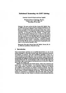
In the Phase Transition setting, each clause φ is generated from n variables (in a set X ) and m binary predicates (in a set P), by first constructing its skeleton ϕs = α1 (x1 , x2 ) ∧ . . . ∧ αn−1 (xn−1 , xn ) (obtained by chaining the n variables through (n − 1) predicates), and then adding to ϕs the remaining (m−n+1) predicates, whose arguments are randomly, uniformly, and without replacement selected from X . Given Λ, a set of L constants, an example, against which checking the subsumption of the generated clause, is built using N literals for each predicate symbol in P, whose arguments are selected uniformly and without replacement from the universe U = Λ × Λ. In such a setting, a matching problem is defined by a 4-tuple (n,m,L,N ). In this experiment, n was set to 4, N was set to 4, m ranges in [4, 7], and L ranges in [4, 7]. For each pair (m, L), an hypothesis and 100 examples (50 positive and 50 negative) were constructed. The results are depicted in Figures 1, 2 and 3, reporting, respectively, the results for all the problems with α = 800, 400, α = 200, 100 and α = 50, 10.

Fig. 1 Approximate subsumption degree for positive (POS) and negative (NEG) examples, with α = 800 (left) and α = 400 (right)

Fig. 2 Approximate subsumption degree for positive (POS) and negative (NEG) examples, with α = 200 (left) and α = 100 (right)

Approximate Relational Reasoning by Stochastic Propositionalization

91

Fig. 3 Approximate subsumption degree for positive (POS) and negative (NEG) examples, with α = 50 (left) and α = 10 (right)

For each problem, the corresponding bars indicate, respectively, the mean of the approximate subsumption degree obtained by matching the clause against the 50 positive and 50 negative examples. As we can see, the mean value obtained over the positive examples is greater than the one obtained over the negative examples, proving that, on this synthetic dataset, the approximate subsumption degree is able to discriminate between positive and negative examples.

3 The Anytime Induction Method Algorithm 1 reports the sketch of the Sprol system, implemented in Yap Prolog 5.1.1, that incorporates ideas of the propositional framework we proposed. Sprol is a population based algorithm where several individual candidate solutions are simultaneously maintained using a constant size population implementing the anytime nature of the algorithm. The population of candidate solutions provides a straightforward means for achieving search diversification and hence for increasing the exploration capabilities of the search process. In our case, the population is made up of candidate generalizations over the training positive examples. In many cases, local minimum are quite common in search algorithms and the corresponding candidate solutions are not typically of sufficiently high quality. The strategy we used to escape from local minimum is a restart strategy that simply re-initialises the search process whenever a local minimum is encountered. Sprol takes as input the set of positive and negative examples of the training set and some user-defined parameters characterizing its approximate and anytime behaviour. In particular, α and β represent the number of renamings of a negative, respectively positive, example to use for the covering test; k is the size of the population; and r is the number of restarts.

92

N. Di Mauro et al.

Algorithm 1. Sprol Input: E + : positive examples; E − : negative examples; α: the parameter for negative coverage; β: the parameter for positive coverage; k: the dimension of the population; r: number of restarts; Output: the hypotheses h 1: C = argmaxE ∈E=E+ ∪E− (|consts(Ei )|); i

2: while E + = ∅ do 3: select a seed e from E + 4: /* select k renamings of e */ 5: Population ← ren(k, e, C); 6: PopPrec ← Population; i ← 0; 7: while i < r do 8: P ← ∅; 9: for each element v ∈ Population do 10: for each positive example e+ ∈ E + do 11: /* select t renamings of e+ */ 12: Ve+ ← ren(t, e+ , C); 13: /* generalization */ 14: P ← P ∪{u|u = v ∩ wi , wi ∈ Ve+ }; 15: Population ← P; 16: /* Consistency check */ 17: for each negative example e− ∈ E − do 18: /* select α renamings of e− */ 19: Ve− ← ren(α, e− , C); 20: for each element v ∈ Population do 21: if v covers an element of Ve− then 22: remove v from Population 23: /* Completeness check */ 24: for each element v ∈ Population do 25: completenessv ← 0; 26: for each positive example e+ ∈ E + do 27: /* select β renamings of e+ */ 28: Ve+ ← ren(β, e+ , C); 29: for each element v ∈ Population do 30: if ∃u ∈ Ve+ s.t. u ∩ v = v then 31: completenessv ← completenessv + 1; 32: i ← i + 1; 33: if |Population| = 0 then 34: /* restart with the previous population */ 35: Population ← PopPrec; 36: else 37: leave in Population the best k generalizations only; 38: PopPrec ← Population; 39: add the best element b ∈ Population to h; 40: remove from E + the positive exs covered by b

As reported in Algorithm 1, Sprol tries to find a set of clauses that covers all the positive examples and no negative one, by using an iterative population based covering mechanism. It sets the initial population made up of k randomly chosen renamings of a positive example (lines 3-5). Then, the elements of the population are iteratively generalized on the positive examples of the training set (lines 9-15). All the generalizations that cover at least one negative example are taken out (lines 16-22), and the quality of each generalization, based on the number of covered positive examples, is calculated (lines 23-31). Finally, best k generalizations are taken into account for the next iteration (line 37). In case of an empty population a restart is generated with the previous population (line 35).

Approximate Relational Reasoning by Stochastic Propositionalization

93

Renamings of an example are generated according to the procedure reported in Algorithm 2, that randomly chooses k renamings of the example E onto the set of constants C. This procedure implements the approximate and anytime nature of the method. Indeed, the parameter k represents at the same time both the approximation degree and the time allocated for the algorithm. The more renamings the algorithm selects, the more accurate generalizations and subsumptions will be, but the more time to compute them will be needed. It is important to note that our approach constructs hypotheses that are only approximately consistent. Indeed, in the consistency check it is possible that there exists a matching between an hypothesis and a negative example. The number α of allowed permutations is responsible of the induction cost as well as of the consistency of the produced hypotheses. An obvious consequence is that the more permutations are allowed, the more consistent are the found hypotheses and, perhaps, the more learning time is required. Algorithm 2. ren(k, E, C) Input: k: the number of renamings; E: the example; C: a set of constants; Output: a set S of renamings of E 1: S ← ∅ 2: for i = 1 to k do 3: S ← S ∪ {R(E){C} }

4 Approximate Relational Clustering Clustering represents a classical problem in knowledge discovery and artificial intelligence whose aim is to find similar groups of objects from a database. Basically, clustering is an unsupervised learning technique used to find a partition of a given set of objects into clusters so that the objects within each cluster are similar to each other. The similarity between objects can be determined using various distance functions. Relational clustering regards grouping relational data (i.e., objects with a first-order description) by using distance measures that are generally more complex than those used in the case of propositional data. Indeed, the generic Euclidean distance cannot be applied to relational data since, in this case, objects are not represented by a feature vector of a fixed number of measurements. In this chapter we used the propositionalization framework introduced in the Section 2 in order to compute the distance between two ground clauses. Other relational distance measures for comparing first-order descriptions concerning supervised and unsupervised learning can be found in [7, 4, 27, 24, 5]. Among all the clustering algorithms, a partitional clustering algorithm, named Partition Around Medoids (PAM) [16] and its variant Supervised Partition Around Medoids (SPAM) [13], have been used for our study.

94

N. Di Mauro et al.

4.1 Definitions and Notations In this section we will use the following terms and notations, as reported in Table 2. • An object (or observation, or datum) x is a single data object used by the clustering algorithm. In our case of relational clustering, it consists of a set of ground literals {l1 , l2 , . . . , ln } whose arguments range over a finite set of constants Ω. • An object set is denoted by X = {x1 , x2 , . . . xn }. • A class governs the objects generation process whose distribution in the objects space is characterized by a probability density specific to the class. In particular, in case we known the class ci the object belongs to, then we can describe the object as a ground horn clause ci ← l1 , l2 , . . . , ln . • A distance measure is a metric on the observation space used to quantify the similarity of objects. Table 2 Notations used for clustering Notation

Description

X = {x1 , . . . , xn } n d(oi , oj ) c Ci μi k C = {C1 , . . . , Ck } J (Ci )

objects in the data set number of objects in the data set distance between objects oi and oj the number of classes in the data set cluster associated with the i-th representative representative of the i-th cluster the number of clusters a clustering solution an objective function that evaluates a clustering solution Ci

Definition 9 (Distance [12]). A distance d(·, ·) is a function that gives a generalized scalar distance between two arguments objects. A distance must have four properties: for all objects a, b and c non-negativity: d(a, b) ≥ 0 reflexivity: d(a, b) = 0 if and only if a = b symmetry: d(a, b) = d(b, a) triangle inequality: d(a, b) + d(b, c) ≥ d(a, c).

4.2 Similarity Measure Measuring the similarity between two objects drawn from the same object space is fundamental for clustering. For computing the distance between objects we adopted the Tanimoto metric [12], that finds most use in taxonomy, where the distance between two sets is defined as

Approximate Relational Reasoning by Stochastic Propositionalization

dT (S1 , S2 ) =

n1 + n2 − 2n12 , n1 + n2 − n12

95

(4)

where n1 and n2 are the numbers of elements in sets S1 and S2 , respectively, and n12 is the number that is in both sets. The value of the Tanimoto distance ranges in [0, 1]; a value close to 0 implies similarity and a value close to 1 implies a dissimilarity among the two descriptor sets compared. Since, in our relational clustering scenario the objects are ground clauses (i.e., sets of literals), we need a method to find the common components (i.e., literals) of the two instances. We use the word “instance” since each clause can be labeled with the class it belongs to, and it can be represented as c ← l 1 , l 2 , . . . , ln . In particular, given two instances E1 : ci ← l11 , l12 , . . . , l1n and E2 : cj ← l21 , l22 , . . . , l2m , and let C = argmaxEi (|consts(Ei )|), then the number of literals in common to E1 and E2 is approximated using the formula reported in Equation 5 α |RE1 ∩ RE2 i | , (5) s∩ (E1 , E2 , α) = i=1 α where RE1 = ren(1, E1 , C) is a fixed renaming of the example E1 , RE2 i ∈ ren(α, E1 , C) is a renaming of the example E2 , and α > 0 is the parameter governing the approximation. In other words, s∩ (E1 , E2 , α) is the mean of the number of common literals in E1 and E2 for each of the α renamings of E2 . Now we can use the Tanimoto metric to define the distance between two instances E1 and E2 as reported in the Equation 6, dT∩ (E1 , E2 , α) =

|E1 | + |E2 | − 2s∩ (E1 , E2 , α) , |E1 | + |E2 | − s∩ (E1 , E2 , α)

(6)

where |Ei | is the number of literals appearing in the instance Ei .

4.3 Approximate Partition Around Medoid A partitional clustering algorithm obtains a single partition of n objects into a set of k clusters by optimizing an objective function. The exhaustive enumeration of all the possible partitions into k sets in order to find the global maximum is too expensive. Hence, partitional clustering algorithms use the following generic schema: 1. randomly choose k representatives for clusters; 2. iteratively improve these initial representatives until the change in the objective function from one iteration to the next drops below a given threshold a. assign each object to the cluster it “fits best” in the current clustering b. compute new cluster representatives using these new assignments One of the most well-known and commonly used partitioning method is the kmedoids clustering algorithm. Unlike other partitioning methods, k-medoids

96

N. Di Mauro et al.

based algorithms are very robust with respect to the existence of outliers (i.e., data points that are very far away from the rest of the data points). In particular, given X = {xi }ni=1 a set of objects, let {μh }kh=1 be the k cluster representatives, named medoids, and li be the cluster assignment of an object xi , where li ∈ L and L = {1, . . . , k}, the goal of the the k-medoids algorithm is to find the best clustering solution C optimizing the objective function J (C). The k-medoids method we used in this chapter is the well-known Partition Around Medoids (PAM) [16] clustering algorithm. In order to find k clusters, PAM finds a representative object μi (medoid) for each cluster. This representative object is meant to be the most centrally located object for each cluster. Once the k medoids have been selected, each non-selected object is grouped with the medoid to which it is the most similar. More precisely, if xj is a non-selected object, and xi is a (selected) medoid, then xj belongs to the cluster represented by xi if d(xj , xi ) = minh=1,...,k d(xj , xh ), where d(xj , xi ) denotes the dissimilarity, or distance, between objects xj and xi . Finally, the quality of the chosen medoids is measured by the average dissimilarity between a non-selected object and the medoid of its cluster. Algorithm 3 reports the main procedure of the PAM method. In order to find k medoids, PAM starts with an arbitrary selection of k objects. Then in each step, a swap between a selected object xi and a non-selected object xh is made, as long as such a swap would result in an improvement of the quality of the clustering. In particular, to calculate the effect of such a swap between xi and xh , PAM computes costs Cih for all non-selected objects xj .

Algorithm 3. PAM Input: D: database of objects Output: k clusters 1: select k representative objects, and mark these objects as medoid and the remaining as non-medoid 2: repeat 3: for all medoid objects Oi do 4: for all non-medoid objects Oh do 5: compute Cih 6: select imin , hmin such that Cimin hmin = mini,h Cih 7: if Cimin hmin < 0 then 8: mark Oi as non-medoid object and Oh as medoid object 9: until convergence criterion is met

4.4 Objective Function Traditional k-medoids clustering algorithm seeks to find k medoids among the objects in the data set minimizing, for a given clustering solution C, the objective function reported in Equation 7,

Approximate Relational Reasoning by Stochastic Propositionalization

tightness(C) =

1  d(xi , μi )), n i=1,...,n

97

(7)

where μi is the medoid of the cluster the object xi belongs to. Hence, PAM starts with a set of clusters containing the medoids of the complete data set, and greedily inserts new objects into this set of clusters while minimizing the above fitness function. Then, it tries to improve the previously obtained clustering by exploring all possible replacements of medoids by non-medoids picking the replacement that enhances the fitness function. If no such fitness improving replacement can be found, PAM terminates. The Algorithm 4 is the proposed approximate relational clustering variant of PAM, named Approximate PAM, that uses the objective function reported in Equation 8. It starts by randomly selecting k medoids and finding the first clustering solution C by associating each non-medoid instance to the cluster whose medoid is more similar. Then, it iteratively tries to swap a medoid with a non-medoid object, exploring all possible replacements, in order to minimize the value of the objective function Jtightness (·, ·). It terminates if no replacement can be found that leads to a clustering with a better (lower) objective value with respect to Jtightness (·, ·). Jtightness (C, α) =

1  dT (xi , μi , α). n i=1,...,n ∩

Algorithm 4. Approximate PAM Input: X = {xi }n i=1 : set of instances (ground clauses) Output: C = {C1 , . . . , Ck }: k clusters 1: randomly select k medoids μi 2: C = {Ci |Ci = {μi }}i=1,...,k 3: for all non-medoid objects xh do 4: /* find the best cluster */ 5: Cj = Cj ∪ {xh } being dT∩ (xh , μj , α) = mint=1,...,k dT∩ (xh , μt , α) 6: V = Jtightness (C, α) 7: repeat 8: randomly select a medoid objects μi 9: randomly select a non-medoid objects xp 10: C = C 11: /* swap μi with xp */ 12: Cp = {xp } 13: mark μi as a non-medoid 14: /* re-clustering */ 15: for all non-medoid objects xh do 16: Cj = Cj ∪ {xh } being dT∩ (xh , μj , α) = mint=1,...,k dT∩ (xh , μt , α) 17: V  = Jtightness (C  , α) 18: if V  < V then 19: C = C 20: V = V 21: until no possible swap improves the optimization of Jtightness (C, α)

(8)

98

N. Di Mauro et al.

4.5 Approximate Supervised Partition Around Medoid While clustering is typically applied in an unsupervised learning framework using a particular error function, supervised clustering [13], on the other hand, deviates from traditional clustering in that it is applied on classified examples with the objective of identifying clusters that have high probability density with respect to a single class. Similar to supervised clustering is semi-supervised clustering that tries to obtain better results by considering a subset of the classified examples optimising the class purity. The goal is to find a clustering by optimising an objective function that takes as input the class label also. The objective functions used for supervised clustering are significantly different from the objective functions used by traditional clustering algorithms. Indeed, supervised clustering algorithms may evaluate a clustering based on the class impurity measured by the percentage of the minority examples in the different clusters. We propose an Approximate variant of the Supervised Partition Around Medoid clustering algorithm (SPAM) [13], named Approximate SPAM, that uses an objective function different from Jtightness (C, α). Indeed, in case of class labeled instances, we can use two other metrics for the evaluation of the clustering solutions, such as purity and entropy. Entropy provides a measure of “goodness” for clusters. Entropy indicates how homogeneous is a cluster. The higher the homogeneity of a cluster the lower the entropy is, and viceversa. The entropy of a cluster containing only one object (perfect homogeneity) is zero. For each cluster Cj in the clustering result C we compute pij , the probability that a member of the cluster Cj belongs to class i as nij , (9) pij = nj where nj is the number of objects contained in the cluster Cj , and nij is the number of data objects of the i-th class that were assigned to the cluster Cj . The entropy of each cluster Cj may be calculated using the following formula c c   nij nij E(Cj ) = − pij log(pij ) = − log , (10) n nj i=1 i=1 j where the sum is taken over all the c classes. The entropy of the entire clustering solution is then defined to be the sum of the individual cluster entropies weighted according to the cluster size: E(C) =

k  nr r=1

n

E(Cj )

(11)

A perfect clustering solution should be the one that leads to clusters that contain objects from only a single class, in which case the entropy will be

Approximate Relational Reasoning by Stochastic Propositionalization

99

zero. In general, the smaller the entropy values, the better the clustering solution is. The purity measures, for each cluster, how many objects belong to its primarily class. The purity of the cluster Cj is defined to be P (Cj ) =

1 max(nij ), nj i

(12)

which is nothing more than the fraction of the overall cluster size that the largest class of objects assigned to that cluster represents. The overall purity of the clustering solution C is obtained as a weighted sum of the individual cluster purities and is given by P(C) =

k  nr r=1

n

P (Cr ).

(13)

In general, the larger the values of purity, the better the clustering solution is. In our Approximate SPAM clustering algorithm we used the objective function reported in the Equation 14 corresponding to the purity of the clustering solution. (14) Jpurity (C, α) = P (C), where α corresponds to the approximation value. In particular, given a set of data objects X , and a number of cluster to form, k, it finds a disjoint k partitioning {Xh }kh=1 of X such that Jpurity (C, α) is maximized.

5 Experiments In order to evaluate the system Sprol, we performed experiments on two real world datasets (Table 3). The classical ILP mutagenesis dataset [30] consists of structural descriptions of molecules. The Mutagenesis dataset has been collected to identify mutagenic activity in a compound based on its molecular structure and is considered to be a benchmark dataset for multi-relational learning. The Mutagenesis dataset consists of the molecular structure of 230 compounds, of which 138 are labelled as mutagenic and 92 as non-mutagenic. The mutagenicity of the compounds has been determined by the Ames Test. The task is to distinguish mutagenic compounds from non-mutagenic ones based on their molecular structure. The Mutagenesis dataset basically consists of atoms, bonds, atom types, bond types and partial charges on atoms. The dataset also consists of the hydrophobicity of the compound (logP), the energy level of the compound’s lowest unoccupied molecular orbital (LUMO), a boolean attribute identifying compounds with 3 or more benzyl rings (I1), and a boolean attribute identifying compounds which are acenthryles (Ia). Ia, I1, logP and LUMO are relevant properties in determining mutagencity.

100

N. Di Mauro et al.

A second dataset has been used to evaluate the clustering algorithms. It is a collection of 353 scientific papers in PostScript (PS) or Portable Document Format (PDF) format, whose first pages layout descriptions were automatically generated by a document layout analysis system [14]. The documents belong to 4 different classes: Elsevier journals, Springer-Verlag Lecture Notes (SVLN) series, Journal of Machine Learning Research (JMLR) and Machine Learning Journal (MLJ). Table 3 Data Sets Data Set Name # examples # classes Mutagenesis Documents

188 353

2 4

All the experiments have been carried out on machine equipped with an Intel(R) Core(TM)2 Duo CPU T7250 @ 2.00GHz and 2GiB RAM @ 667MHz.

5.1 Induction Task In this section we report the results obtained by the Sprol system when applied to the mutagenesis dataset. The size of the population has been set to 50, the parameter α to 50, the parameter β to 50, and making 5 restarts. As measures of the performance, we used predictive accuracy and execution time. Results have been compared to those obtained by running, on both the same machine and dataset, the system Progol [22]. A 10-fold cross-validation produced the results reported in Table 4, averaged over the 10-folds, where Table 4 Execution time (in seconds) and accuracy of Progol and Sprol on the mutagenesis dataset. Progol SPROL Time Accuracy Time Accuracy M1 M2 M3 M4 M5 M6 M7 M8 M9 M10 Mean

330.76 479.03 535.95 738.54 699.90 497.08 498.22 584.00 511.88 587.18 546.25

84.21 78.95 84.21 68.42 89.47 78.95 84.21 78.95 68.42 82.35 79.81

56.73 41.15 48.51 63.67 55.56 53.55 71.97 56.29 50.44 65.63 56.35

57.89 89.47 73.68 84.21 84.21 78.49 84.21 89.47 83.33 70.59 79.60

Approximate Relational Reasoning by Stochastic Propositionalization

101

we can note that there is an evident improvement of the execution time with respect to Progol obtaining a comparable predictive accuracy of the learned theory. A second experiment, whose results are reported in Table 5, has been made in order to evaluate how the behaviour of the algorithm change by altering parameters k, α and β. Table 5 Results on parameter settings.

k = 50 α = 50 β = 50 k = 75 k = 100 β = 40 β = 50 α = 50 k = 50 β = 60 β = 100 α = 40 α = 50 β = 50 k = 50 α = 60

Time Accuracy 75.49 71.14 96.80 75,35 117.29 71.67 78.84 78.67 75.49 71.14 74.39 76.85 114 78.02 75.49 70.19 75.49 71.14 56.35 79.6

As we can see in Table 5, the first row reports the case in which we fixed α and β and letting k to change. Obviously, taking more elements in the population makes grow the execution time. Furthermore, the second and the third row show that changing β does not change the accuracy of the theory. On the contrary α seems to be more important than β in improving the system performances. A further investigation of this behaviour deserves a more accurate experiment on an ad-hoc artificial dataset.

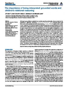
5.2 Clustering Task In this section we report the results obtained by the Approximate PAM and Approximate SPAM on the mutagenesis (Figures 4,5, and 6) and documents (Figures 7,8, and 9) dataset with the approximation parameter α taking values 20, 50, and 100. As we can see, for both the dataset Approximate PAM obtains clustering solutions with a better tightness, while Approximate SPAM obtains clustering solutions with a better purity. In general, good solutions are obtained when we choose a high value for the number of k clusters, since in this case the system is more free to partition the objects in the clusters. As expected the entropy values obtained by Approximate SPAM are lower than that obtained by Approximate PAM, since the former tries to find a good solution by optimizing the clusters’ purity. Finally, the execution of the algorithm with high values of the α parameter shows an increment about the quality of the clustering solution, even if with small values good results have been obtained.

102

N. Di Mauro et al.

Fig. 4 Tightness, Purity, Entropy and Iterations values obtained by Approximate PAM and Approximate SPAM for the Mutagenesis dataset with α = 20

6 Discussion and Conclusion Various strategies have been proposed in order to overcome the limitation imposed by the inborn complexity of most real-word applications whose descriptions involve many relationships. One of the classical approaches consists in the reformulation of the relational learning in a propositional one followed by the application of well known propositional learners and by the mapping back in relational form of the resulting hypotheses. During the reformulation, a fixed set of structural features is built from relational background knowledge and the structural properties of the individuals occurring in the examples. In such a process, each feature is defined in terms of a corresponding program clause whose body is made up of a set of literals derived from the relational background knowledge. When the clause defining the feature is called for a particular individual (i.e., if its argument is bound to some example identifier) and this call succeeds at least once, the corresponding boolean feature is defined to be true for the given example; otherwise, it is defined to be false. Examples of systems that implement such kind of propositionalization process are LINUS [20], and its extensions DINUS [19] and SINUS [18], and RSD [21].

Approximate Relational Reasoning by Stochastic Propositionalization

103

Fig. 5 Tightness, Purity, Entropy and Iterations values obtained by Approximate PAM and Approximate SPAM for the Mutagenesis dataset with α = 50

Alternative approaches avoid the reformulation process and apply propositionalization directly on the original FOL context: the relational examples are flattened by substituting them with all (or a subset of) their matchings with a pattern. To this concern, it was noted [28, 33, 2] that a most suitable setting for supervised relational learning is that of multiple instance problems (MIP), first introduced by Dietterich [11], where each example consists of a set of literals (instances) built on a same predicate symbol. The multiple instances representation is an extension that offers a good trade-off between the expressive power of relational learning and the low complexity of propositional learning. Unfortunately, most of the existing inductive learning systems are not able to face efficiently with this problem. In some cases the learning system has an incomplete knowledge about each training example: It does not know the features vector but it only knows that each example can be represented by means of one (or more) potential feature vectors (a bag of instances). Following this idea, [29, 33, 2] proposed a multi-instance propositionalization. In such a framework each relational example is reformulated in its multiple matchings with a pattern (a formula of the initial hypotheses space that can be built from the training data or provided by the user). After the

104

N. Di Mauro et al.

Fig. 6 Tightness, Purity, Entropy and Iterations values obtained by Approximate PAM and Approximate SPAM for the Mutagenesis dataset with α = 100

reformulation, each initial observation corresponds to many feature vectors and the search for hypotheses may be re-casted in this propositional representation as the search for rules that cover at least one instance per observation. Consequently, the learning task is no longer to induce a hypothesis that is consistent with all the feature vectors reformulated but a hypothesis that covers at least one reformulated example of each positive initial training example and no reformulated example of any negative initial training example. Specifically, the approach proposed in [33] consists in limiting the number of possible mappings by means of a selective mapping and then searching inductive generalizations in the hypotheses space defined by the selected mapping type. The type of mapping, i.e. the relevant propositionalization pattern, is provided by the user/expert and represents a (strong) bias which allows to dramatically reduce the matching space. On the contrary, in [29] the propositionalization process is done through a stochastic selection on each example of a user-defined number of example matchings with the pattern, which allows to reduce the dimensionality of the reformulated problem. In other words, for each example it is constructed the set of a user-defined number of hypotheses covering the example and not covering any example belonging to other classes. Then a representative of such a set for each example is learned

Approximate Relational Reasoning by Stochastic Propositionalization

105

Fig. 7 Tightness, Purity, Entropy and Iterations values obtained by Approximate PAM and Approximate SPAM for the Documents dataset with α = 20

that classifies unseen examples via a nearest-neighbour-like process. Finally, [2] proposed a method that selectively propositionalizes the relational data by interleaving attribute-value reformulation and algebraic resolution avoiding, as much as possible, the generation of reformulated data which are not relevant with respect to the discrimination task and obtaining a reformulated learning problem of tractable size. The obtained set of attribute-value instances is then used to solve the initial relational problem by applying a data-driven strategy. Based on this kind of more suitable propositionalization and on the existing effective and efficient techniques for feature selection, [1] proposed an extension of classical feature selection methods for coping with the problem of relational data by firstly transforming the original relational data in propositional ones by means of a multi-instance propositionalization and successively applying methods for feature selection on such a new transformation. In [17] the authors propose a stochastic algorithm to automatically derive features from background knowledge. The algorithm conducts a top-down search for first-order clauses, where each clause represents a binary feature. These features are used instead of relations in a subsequent induction step. In [3] has been presented a work on clustering relational data by using propo-

106

N. Di Mauro et al.

Fig. 8 Tightness, Purity, Entropy and Iterations values obtained by Approximate PAM and Approximate SPAM for the Documents dataset with α = 50

sitionalization. They propositionalize the relational data using randomly generated first-order rules, which are then converted into boolean features, based on their coverage. Then the resulting propositional dataset is clustered using a standard propositional clustering algorithm. It is different from our approach since it is based on checking the coverage of the generated rule (computationally expensive). Furthermore it does not cluster directly the relational data but its propositional description. Efficient multi-relational data mining algorithms have to tackle the problem of selecting the best search method for exploring the hypotheses space and the problem of reducing the complexity of the coverage procedure that assesses the validity of the learned theory against the training examples. A way of tackling the complexity of this kind of learning systems is to use a propositional method, that reformulates a multi-relational learning problem into an attribute-value one. In this chapter we presented a population based algorithm able to efficiently solve multi-relational problems, and a relational clustering algorithm, by using an approximate propositional method. The result of an empirical evaluation on two real-world datasets of the proposed techniques is very promising and proves the validity of the method.

Approximate Relational Reasoning by Stochastic Propositionalization

107

Fig. 9 Tightness, Purity, Entropy and Iterations values obtained by Approximate PAM and Approximate SPAM for the Documents dataset with α = 100

As a future work, we want to investigate the behaviour of the algorithm in the case of approximate completeness. In particular, we want to use the approximate subsumption degree between clauses in order to induce theories when noisy or uncertain data are available.

References ´ Matwin, S.: A dynamic approach to dimensionality reduction in 1. Alphonse, E., relational learning. In: Hacid, M.-S., Ra´s, Z.W., Zighed, D.A., Kodratoff, Y. (eds.) ISMIS 2002. LNCS (LNAI), vol. 2366, pp. 255–679. Springer, Heidelberg (2002) 2. Alphonse, E., Rouveirol, C.: Lazy propositionalization for relational learning. In: Horn, W. (ed.) Proc. of the 14th European Conference on Artificial Intelligence, pp. 256–260. IOS Press, Amsterdam (2000) 3. Anderson, G., Pfahringer, B.: Clustering relational data based on randomized propositionalization. In: Blockeel, H., Ramon, J., Shavlik, J., Tadepalli, P. (eds.) ILP 2007. LNCS (LNAI), vol. 4894, pp. 39–48. Springer, Heidelberg (2008) 4. Bisson, G.: Learning in FOL with a similarity measure. In: Proceedings of the 10th National Conference on Artificial Intelligence, pp. 82–87 (1992)

108

N. Di Mauro et al.

5. Blockeel, H., Raedt, L.D., Ramon, J.: Top-down induction of clustering trees. In: Proceedings of the 15th International Conference on Machine Learning, pp. 55–63. Morgan Kaufmann, San Francisco (1998) 6. Boddy, M., Dean, T.L.: Deliberation scheduling for problem solving in timeconstrained environments. Artificial Intelligence 67, 245–285 (1994) 7. Bohnebeck, U., Horv´ ath, T., Wrobel, S.: Term comparisons in first-order similarity measures. In: Proceedings of the 8th International Workshop on Inductive Logic Programming, pp. 65–79. Springer, Heidelberg (1998) 8. Bratko, I.: Prolog programming for artificial intelligence, 3rd edn. AddisonWesley Longman Publishing Co., Amsterdam (2001) 9. Di Mauro, N., Basile, T.M.A., Ferilli, S., Esposito, F.: Approximate reasoning for efficient anytime induction from relational knowledge bases. In: Greco, S., Lukasiewicz, T. (eds.) SUM 2008. LNCS (LNAI), vol. 5291, pp. 160–173. Springer, Heidelberg (2008) 10. Di Mauro, N., Basile, T.M.A., Ferilli, S., Esposito, F.: Stochastic propositionalization for efficient multi-relational learning. In: An, A., Matwin, S., Ra´s, Z.W., ´ ezak, D. (eds.) Foundations of Intelligent Systems. LNCS (LNAI), vol. 4994, Sl  pp. 78–83. Springer, Heidelberg (2008) 11. Dietterich, T.G., Lathrop, R.H., Lozano-Perez, T.: Solving the multiple instance problem with axis-parallel rectangles. Artificial Intelligence 89(1-2), 31– 71 (1997) 12. Duda, R.O., Hart, P.E., Stork, D.G.: Pattern Classification. Wiley Interscience, Hoboken (2000) 13. Eick, C.F., Zeidat, N., Zhao, Z.: Supervised clustering: Algorithms and benefits. In: ICTAI 2004: Proceedings of the 16th IEEE International Conference on Tools with Artificial Intelligence, pp. 774–776. IEEE Computer Society Press, Los Alamitos (2004) 14. Esposito, F., Ferilli, S., Basile, T.M.A., Di Mauro, N.: Machine learning for digital document processing: From layout analysis to metadata extraction. In: Marinai, S., Fujisawa, H. (eds.) Machine Learning in Document Analysis and Recognition. Studies in Computational Intelligence, vol. 90, pp. 105–138. Springer, Heidelberg (2008) 15. Giordana, A., Botta, M., Saitta, L.: An experimental study of phase transitions in matching. In: Thomas, D. (ed.) Proceedings of the 16th International Joint Conference on Artificial Intelligence. Morgan Kaufmann, San Francisco (1999) 16. Kaufman, L., Rousseeuw, P.: Finding groups in data: an introduction to cluster analysis. John Wiley and Sons, Chichester (1990) 17. Kramer, S., Pfahringer, B., Helma, C.: Stochastic propositionalization of nondeterminate background knowledge. In: Proceedings of the 8th International Workshop on Inductive Logic Programming, pp. 80–94. Springer, Heidelberg (1998) 18. Krogel, M.A., Rawles, S., Zelezny, F., Flach, P., Lavrac, N., Wrobel, S.: Comparative evaluation of approaches to propositionalization. In: Horv´ ath, T., Yamamoto, A. (eds.) ILP 2003. LNCS (LNAI), vol. 2835, pp. 194–217. Springer, Heidelberg (2003) 19. Lavrac, N., Dzeroski, S.: Inductive Logic Programming: Techniques and Applications. Ellis Horwood, New York (1994) 20. Lavrac, N., Dzeroski, S., Grobelnik, M.: Learning nonrecursive definitions of relations with linus. In: Proceedings of the European Working Session on Machine Learning, pp. 265–281. Springer, Heidelberg (1991)

Approximate Relational Reasoning by Stochastic Propositionalization

109

ˇ 21. Lavraˇc, N., Zelezn´ y, F., Flach, P.A.: RSD: Relational subgroup discovery through first-order feature construction. In: Matwin, S., Sammut, C. (eds.) ILP 2002. LNCS (LNAI), vol. 2583, pp. 149–165. Springer, Heidelberg (2003) 22. Muggleton, S.: Inverse Entailment and Progol. New Generation Computing, Special issue on Inductive Logic Programming 13(3-4), 245–286 (1995) 23. Muggleton, S., De Raedt, L.: Inductive logic programming: Theory and methods. Journal of Logic Programming 19/20, 629–679 (1994) 24. Nienhuys-Cheng, S.-H.: Distances and limits on herbrand interpretations. In: Proceedings of the 8th International Workshop on Inductive Logic Programming, pp. 250–260. Springer, Heidelberg (1998) 25. Plotkin, G.D.: A note on inductive generalization. In: Meltzer, B., Michie, D. (eds.) Machine Intelligence, ch. 8, vol. 5, pp. 153–163. Edinburg Univ. Press (1970) 26. Raedt, L.D.: Attribute value learning versus inductive logic programming: The missing links (extended abstract). In: Page, D.L. (ed.) ILP 1998. LNCS, vol. 1446, pp. 1–8. Springer, Heidelberg (1998) 27. Sebag, M.: Distance induction in first order logic. In: Proceedings of the 7th International Workshop on Inductive Logic Programming, pp. 264–272. Springer, Heidelberg (1997) 28. Sebag, M., Rouveirol, C.: Induction of maximally general clauses consistent with integrity constraints. In: Wrobel, S. (ed.) Proceedings of the 4th International Workshop on Inductive Logic Programming. GMD-Studien, vol. 237, pp. 195– 216. Gesellschaft f¨ ur Mathematik und Datenverarbeitung MBH (1994) 29. Sebag, M., Rouveirol, C.: Tractable induction and classification in first order logic via stochastic matching. In: 15th International Join Conference on Artificial Intelligence, pp. 888–893. Morgan Kaufmann, San Francisco (1997) 30. Srinivasan, A., Muggleton, S., King, R.: Comparing the use of background knowledge by inductive logic programming systems. In: Raedt, L.D. (ed.) Proceedings of the 5th International Workshop on Inductive Logic Programming, pp. 199–230. Springer, Heidelberg (1995) 31. Ullman, J.: Principles of Database and Knowledge-Base Systems, vol. I. Computer Science Press (1988) 32. Zilberstein, S., Russell, S.: Approximate reasoning using anytime algorithms. Imprecise and Approximate Computation 318, 43–62 (1995) 33. Zucker, J.-D., Ganascia, J.-G.: Representation changes for efficient learning in structural domains. In: Proceedings of 13th International Conference on Machine Learning, pp. 543–551. Morgan Kaufmann, San Francisco (1996)