nonlinear operator equations in L2(0,1), for which the forward operator is a compo- sition of a linear ... Email: hofmannb @ mathematik.tu-chemnitz.de. 1 ...... http://www.mathematik.tu-chemnitz.de/preprint/2005/PREPRINT_09.html. [7] Engl ...
Approximate source conditions in Tikhonov-Phillips regularization and consequences for inverse problems with multiplication operators Bernd Hofmann
∗
Abstract The object of this paper is threefold. First, we investigate in a Hilbert space setting the utility of approximate source conditions in the method of Tikhonov-Phillips regularization for linear ill-posed operator equations. We introduce distance functions measuring the violation of canonical source conditions and derive convergence rates for regularized solutions based on those functions. Moreover, such distance functions are verified for simple multiplication operators in L 2 (0, 1). The second aim of this paper is to emphasize that multiplication operators play some interesting role in inverse problem theory. In this context, we give examples of nonlinear inverse problems in natural sciences and stochastic finance that can be written as nonlinear operator equations in L2 (0, 1), for which the forward operator is a composition of a linear integration operator and a nonlinear superposition operator. The Fréchet derivative of such a forward operator is a composition of a compact integration and a non-compact multiplication operator. If the multiplier function defining the multiplication operator has zeros, then for the linearization an additional illposedness factor arises. By considering the structure of canonical source conditions for the linearized problem it could be expected that different decay rates of multiplier functions near a zero, for example the decay as a power or as an exponential function, would lead to completely different ill-posedness situations. As third we apply the results on approximate source conditions to such composite linear problems in L2 (0, 1) and indicate that only integrals of multiplier functions and not the specific character of the decay of multiplier functions in a neighborhood of a zero determine the convergence behavior of regularized solutions.
MSC2000 subject classification: 47A52, 65J20, 47H30, 47B33, 65R30 Keywords: Inverse and ill-posed problems, multiplication operator, superposition operator, Tikhonov-Phillips regularization, source conditions, convergence rates, distance function Department of Mathematics, Chemnitz University of Technology, D-09107 Chemnitz, Germany. Email: hofmannb @ mathematik.tu-chemnitz.de ∗
1
1
Introduction
Let X and Y be infinite dimensional Hilbert spaces, where k · k denotes the generic norm in both spaces. We are going to study linear operator equations Ax = y
(x ∈ X, y ∈ Y )
(1)
with bounded linear operators A : X → Y which are assumed to be injective with a non-closed range R(A). This implies an unbounded inverse A−1 : R(A) ⊂ Y → X and leads to ill-posed equations (1). Moreover, we consider nonlinear inverse problems written as operator equations F (x) = y
(x ∈ D(F ) ⊂ X, y ∈ Y ),
(2)
where the nonlinear forward operator F : D(F ) ⊂ X → Y has a closed, convex domain and is assumed to be continuous. If F is smoothing enough, in particular if F is compact and weakly closed, then local ill-posedness of equations (2) at the solution point x0 ∈ D(F ) in the sense of [19, definition 2] arises. If the nonlinear operator F is differentiable at the point x0 and F 0 (x0 ) expresses the corresponding Fréchet or Gâteaux derivative, then linearizations of the nonlinear operator equation (2) at the point x0 are linear operator equations of the form (1) with A = F 0 (x0 ). Then the ill-posedness of the nonlinear problem (2) carries over to the linearized problem (1) and a regularization is required for the stable approximate solution of such problems. We focus here on the Tikhonov-Phillips regularization method. In section 2 we investigate the approaches of general source conditions and approximate source conditions and their interplay for obtaining convergence rates in Tikhonov-Phillips regularization of linear equations (1). The first approach is widely discussed in the recent literature on linear ill-posed problems. For the second approach we introduce distance functions d(R) measuring the violation of canonical source conditions on balls with radius R. In detail we study three types of decay rates of d(R) → ∞ as R → ∞ and corresponding convergence rates in regularization. Moreover, we apply the results of section 2 in section 3 to pure multiplication operators M mapping in X = Y = L2 (0, 1) defined as [M x] (t) = m(t) x(t)
(0 ≤ t ≤ 1)
(3)
with appropriate multiplier functions m. Section 4 presents three examples of inverse problems from natural sciences and stochastic finance that lead to ill-posed nonlinear equations (2) with composite nonlinear forward operators F = N ◦ J mapping in L2 (0, 1), where N is a nonlinear Nemytskii operator and J defined as Zs [J x] (s) = x(t) dt (0 ≤ s ≤ 1) (4) 0
is the simple integration operator which is compact in L2 (0, 1). In all three examples we have derivatives F 0 (x0 ) = B for x0 ∈ D(F ), where B = M ◦J is a compact composite linear operator mapping in L2 (0, 1). If the multiplier functions m defining the multiplication operator (3) have essential zeros, then an additional ill-posedness factor occurs. In this context, a study on the influence of varying multiplier functions m in section 5 is based on the distance functions d(R) and completes the paper. 2
2
General and approximate source conditions for convergence rates in Tikhonov-Phillips regularization
We begin our studies with the consideration of ill-posed linear operator equations (1), for which the stable approximate solution requires regularization methods. A standard regularization approach is the classical Tikhonov-Phillips method (see, e.g., [3], [5, chapter 6], [7, chapter 5], [9], [23], [24], [26] and [36]), where regularized solutions xα depending on a regularization parameter α > 0 are obtained by solving the extremal problem kA x − yk2 + α kxk2 −→ min ,
subject to x ∈ X.
(5)
Let x0 ∈ X be the solution of equation (1), which is uniquely determined for the perfect right-hand side y = Ax0 ∈ Y because of the injectivity of A. Instead of y we assume to know the noisy data element y δ ∈ Y with noise level δ > 0 and ky δ − yk ≤ δ. We will distinguish regularized solutions xα = (A∗ A + αI)−1 A∗ y = A∗ (A A∗ + αI)−1 y
(6)
in the case of noiseless data and xδα = (A∗ A + αI)−1 A∗ y δ in the case of noisy data that represent the uniquely determined minimizers of the extremal problem (5) for the elements y and y δ , respectively. In the sequel we call the noiseless error function f (α) := kxα − x0 k = kα (A∗ A + αI)−1 x0 k
(α > 0)
(7)
profile function for fixed A and x0 . In combination with the noise level δ this function determines the total regularization error of Tikhonov-Phillips regularization e(α) := kxδα − x0 k ≤ kxα − x0 k + kxδα − xα k = f (α) + k (A∗ A + αI)−1 A∗ (y δ − y)k (8) with the estimate
δ e(α) ≤ f (α) + √ . 2 α
The inequality (9) is a consequence of the spectral inequality k (A∗ A + αI)−1 A∗ k ≤
following from
√ λ λ+α
≤
1 √ 2 α
(9) 1 √ 2 α
for all λ ≥ 0 and α > 0 in the sense of [7, p.45, formula (2.48)].
Note that lim f (α) = 0 for all x0 ∈ X as proven by using spectral theory for general α→0
linear regularization schemes in [7, p.72, theorem 4.1] (see also [37, p.45, theorem 5.2]), but the decay rate of f (α) → 0 as α → 0 depends on x0 and can be arbitrarily slow (see [34] and [7, proposition 3.11]). However, the analysis of profile functions (7) expressing the relative smoothness of x0 with respect to the operator A yields convergence rates of regularized solutions. For a rather general discussion of this topic we refer to [6]. In this 3
section we first briefly recall the standard approach for analyzing the behavior of f (α) exploiting general source conditions imposed on x0 and then we present an alternative theoretical approach using functions d measuring how far the element x0 is away from the source condition x0 = A ∗ v 0 (v0 ∈ Y, kv0 k ≤ R0 ). (10) It is well-known that (10) would imply
f (α) = kα (A∗ A + αI)−1 A∗ v0 k ≤
√
(11)
α R0
and with (9) for the a priori parameter choice α(δ) ∼ δ the convergence rate �√ � kxδα(δ) − x0 k = O δ as δ → 0.
(12)
The source condition (10) and the resulting convergence rate (12) are considered as canonical in this paper, since the compliance of a condition (10) seems to be a caesura in the variety of possible relative smoothness properties of x0 with respect to A and plays also some role in the regularization theory of nonlinear ill-posed operator equations (2), where the convergence rate (12) can be obtained if A∗ is replaced by the adjoint F 0 (x0 )∗ of the Fréchet derivative of the forward operator F at the point x0 (see [7, chapter 10]). There are different reasons for an element x0 not to satisfy the canonical source condition (10). In the literature frequently the case is mentioned where A is infinitely smoothing and x0 has to be very smooth (e.g. analytic) to satisfy (10). But also for finitely smoothing A and/or smooth x0 (10) can be injured if x0 does not satisfy corresponding (e.g. boundary) conditions required for all elements that belong to the range R(A∗ ). So it is rather natural for an element x0 ∈ X not to fulfill (10). To obtain convergence rates nevertheless, in the recent years general source conditions x0 = ϕ(A∗ A) w
(13)
(w ∈ X)
were used sometimes in combination with variable Hilbert scales (see, e.g., [11], [21], [22], [27], [30], [32] and [35]). In this context, the generator functions with
ϕ(t) (0 < t ≤ t)
t ≥ kAk2
are assumed to be index functions as used in [29], where we call such function ϕ index function if it is positive, continuous and strictly increasing with lim ϕ(t) = 0. Considerat→0
tions in [29] and [31] yield the following proposition. Proposition 2.1 Provided that the index function ϕ(t) is concave for 0 < t ≤ tˆ with some positive constant tˆ ≤ t, then the profile function (7) satisfies an estimate f (α) = kα (A∗ A + αI)−1 ϕ(A∗ A) wk ≤ K ϕ(α) kwk
(0 < α ≤ α)
(14)
for some α > 0 and a constant K ≥ 1 which is one for tˆ = t. Moreover, we have δ e(α) ≤ K ϕ(α) kwk + √ 2 α for the total regularization error. 4
(0 < α ≤ α)
(15)
Under the assumption of proposition 2.1 we can discuss convergence rates for the Tikhonov-Phillips regularization based on general source conditions (13). For any index function ϕ the auxiliary function √ Θ(t) := t ϕ(t) (0 < t ≤ t) is again an index function. The inverse function Θ−1 , which exists in a neighborhood of zero, is also an index function. Now, for sufficiently small δ > 0 the a priori choice of the regularization parameter α = α(δ) (0 < δ ≤ δ) based on the equation δ if kwk > 0 is available kwk Θ(α) = (16) Cδ with a fixed constant C > 0 otherwise is well-defined and satisfies the limit condition lim α(δ) = 0. The parameter choice (16) δ→0
can be rewritten as kxδα(δ)
δ √ 2 α
=
ϕ(α) 2C
− x0 k ≤
�
−1
with α = Θ (Cδ). Then by formula (15) we obtain 1 Kkwk + 2C
�
ϕ Θ−1 (Cδ)
�
(0 < δ ≤ δ)
with δ = Θ(α)/C and the index function ϕ ◦ Θ−1 characterizes the rate of convergence of regularized solutions. In particular, if we set C = 1/kwk and if moreover ϕ(t) is concave for 0 < t ≤ kAk2 , then we have K = 1 and the error estimate � � �� δ 3 −1 δ (0 < δ ≤ δ = Θ(α)kwk), kxα(δ) − x0 k ≤ kwk ϕ Θ 2 kwk which is the result of corollary 5 in [29]. Moreover, the following proposition can be proven. Proposition 2.2 Under the assumption of proposition 2.1 we have the convergence rate �� kxδα(δ) − x0 k = O ϕ Θ−1 (δ) as δ → 0 (17) of Tikhonov-Phillips regularization for the a priori choice (16) of the regularization parameter α.
We should remark that the concavity of ϕ in a right neighborhood of zero does not imply the concavity of the rate function ϕ ◦ Θ−1 . However, for concave and sufficiently smooth ϕ the modified function ϕ2 ◦ (Θ2 )−1 is concave in such a case. Therefore ϕ ◦ Θ−1 is an order optimal convergence rate as the following proposition asserts. Proposition 2.3 The rate (17) obtained for Tikhonov-Phillips regularization under the assumption of proposition 2.1 is an order optimal convergence rate provided that ϕ(t) is twice differentiable and ln(ϕ(t)) is concave for 0 < t ≤ kAk2 .
5
Note the the assertions of the propositions 2.2 and 2.3 are direct consequences of results formulated in [29] and [30] for a more general regularization setting. Special case 1 (Hölder convergence rates) For all parameters κ with 0 < κ ≤ 1 the index functions ϕ(t) = tκ (0 < t < ∞) (18) 2
1
are concave, where Θ(t) = tκ+ 2 , and with the a priori parameter choice α(δ) ∼ δ 2κ+1 according to (16) from (17) we have the order optimal convergence rate � 2κ � kxδα(δ) − x0 k = O δ 2κ+1 as δ → 0 . (19) 1
Due to the equation R(A∗ ) = R((A∗ A) 2 ) ([7, proposition 2.18]) a source condition of type (13) with index function ϕ from (18) implies in the case κ = 12 always a condition of type (10) and vice versa. Hence, in this case the general source condition and the canonical source condition coincide. Higher convergence rates that are not of interest in this paper are obtained for 21 < κ ≤ 1, but as a consequence of the qualification � one � of 2
Tikhonov-Phillips regularization method only rates up to a saturation level O δ 3 can be reached (see, e.g., [9], [33]). On the other hand, weaker assumptions compared to (10) correspond with the parameter interval 0 < κ < 12 yielding in a natural manner also slower convergence rates compared to (12). Special case 2 (Logarithmic convergence rates) For all parameters p > 0 the index functions 1 ��p ϕ(t) = (0 < t ≤ t = 1/e) (20) ln 1t are concave on the subinterval 0 < t ≤ tˆ = e−p−1 (see example 1 in [29]). Moreover, straightforward calculations show that ln(ϕ(t)) is even concave on the whole domain 0 < t ≤ 1e . If the operator A is scaled such that kAk2 ≤ 1e , then the propositions 2.2 and 2.3 apply. Using the a priori parameter choice α(δ) = c0 δ χ (0 < χ < 2)
(21)
we obtain for sufficiently small δ > 0 as a consequence of the estimates (9) and (14) and with δ ζ = O (ln(1/δ))−p ) as δ → 0 for all ζ > 0 and p > 0 the convergence rate ! 1 δ ��p as δ → 0 . (22) kxα(δ) − x0 k = O ln 1δ
Note that the simply structured parameter choice (21) asymptotically for δ → 0 overestimates the values α(δ) selected by solving the equation (16). Nevertheless, the convergence rate (22) implies for the choice (21) also the order optimal rate (17) as already mentioned in [22] and [29].
The results of proposition 2.2 can also be extended to non-concave index functions ϕ if an estimate (14) is shown otherwise (see also [6, proposition 3.3]). This is the case when 6
ϕ(t) t
is non-increasing for 0 < t ≤ tˆ and some tˆ > 0 or ϕ = ϕ1 + ϕ2 is the sum of a concave index function ϕ1 and a nonnegative Lipschitz continuous function ϕ2 with lim ϕ2 (t) = 0 t→0 For example, every index function ϕ which is operator monotone is characterized by such a sum (see [28] and [31] for more details). Let us note that, for given x0 ∈ X and A, the index function ϕ satisfying a general source condition (13) is not uniquely determined. We now present an alternative approach that works with a distance function d. This function measuring the violation of canonical source condition is uniquely determined for given x0 and A and expresses the relative smoothness of x0 with respect to A in a unique manner. The approach is based on the following lemma 2.4 formulated and proved in [5, theorem 6.8]. This lemma is also basic for the results of the paper [21]. Lemma 2.4 If we introduce the distance function d(R) := inf {kx0 − A∗ vk : v ∈ Y, kvk ≤ R},
(23)
then we have f (α) = kxα − x0 k ≤
p √ (d(R))2 + αR2 ≤ d(R) + α R
(24)
for all α > 0 and R ≥ 0 as an estimate from above for the profile function of regularized solutions in Tikhonov-Phillips regularization. Evidently, for every x0 ∈ X the nonnegative distance function d(R) depending on the radius R ∈ [0, ∞) is well-defined and non-increasing with lim d(R) = 0 as a consequence R→∞
R(A∗ )
of the injectivity of A and = X. Properties concerning the fact that source conditions are valid quite general in such approximate manner were also studied in a more general context in the recent book [4]. In the sequel let x0 ∈ X be a fixed element. The following lemma verifies some more details concerning elements v {R} ∈ X with kv {R} k = R and d(R) = kx0 − A∗ v {R} k. Beforehand we note that d(R) > 0 for all R ≥ 0 if x0 6∈ R(A∗ ). In the case (10), however, we have d(R) = 0 for R ≥ R0 . This case, x0 ∈ R(A∗ ), yielding the canonical convergence rate (12) will not be of interest in the sequel. Lemma 2.5 Let x0 6∈ R(A∗ ). Then for every R > 0 there is a uniquely determined element v {R} ∈ Y orthogonal to the null-space of A∗ with kv {R} k = R and d(R) = kx0 − A∗ v {R} k.
(25)
Moreover, there is a one-to-one correspondence λ = λ(R) between R ∈ (0, ∞) and λ ∈ (0, ∞) such that A∗ v {R} is a regularized solution xα according to (6) with regularization parameter α = λ(R) and d(R) = f (λ(R)). (26) Proof: The Lagrange multiplier method for solving the extremal problem kx0 − A∗ vk2 → min,
subject to kvk2 ≤ R2 7
(27)
yields for all λ > 0 uniquely determined elements vλ = (AA∗ + λI)−1 A x0 = A (A∗ A + λI)−1 x0
(28)
orthogonal to the null-space of A∗ minimizing L(v, λ) = kx0 − A∗ vk2 + λ(kvk2 − R2 ) → min,
subject to v ∈ Y,
where (vλ , λ) is a saddle point of the Lagrange functional L(v, λ). Whenever a value λ > 0 satisfies the equation kvλ k = R, then the element vλ is a solution of (27). It is well-known that for injective A and x0 6∈ R(A∗ ) the function ψ(λ) = kvλ k is continuous and strictly decreasing for λ ∈ (0, ∞) with lim ψ(λ) = ∞ and lim ψ(λ) = 0. This ensures λ→0
λ→∞
the existence of a bijective mapping λ = λ(R) of the interval (0, ∞) onto itself such that kvλ(R) k = R . Obviously, we have for all λ > 0 as a consequence of the formulae (28) and (6) the equations A∗ vλ = A∗ (AA∗ + λI)−1 Ax0 = xλ .
Then by setting v {R} := vλ(R) we obtain (25) and (26). This completes the proof. The decay rate of the distance function d(R) → 0 as R → ∞ and the decay rate of the profile function f (α) → 0 as α → 0 both characterize the relative smoothness of x0 with respect to A. The cross-connection is clearly indicated by the equation (26), but the required bijective function λ(R) is not known a priori. On the other hand, lemma 2.4 allows us to estimate f (α) from above by using appropriate settings R := R(α). We are going to analyze three typical situations for the decay of the distance function d in the following: Situation 1 (logarithmic type decay) If d(R) decreases to zero very slowly as R → ∞, the resulting rate for f (α) → 0 as α → 0 is also very slow. Here, we consider the family of distance functions K d(R) ≤ (R ≤ R < ∞) (29) (ln R)p for some constants R > 0, K > 0 and for parameters p > 0. By setting R :=
1 ακ
1 (0 < κ < ) 2
and taking into account that α = O (1/(ln(1/α)p ) as α → 0 we have from (24) and (29) ! 1 �p f (α) = O as α → 0. ln α1
Then by using the a priori parameter choice (21) we obtain the same convergence rate (22) as derived for general source conditions with index function (20) in special case 2. Situation 2 (power type decay) If d(R) behaves as a power of R, i.e., d(R) ≤
K
(R ≤ R < ∞)
γ
R 1−γ 8
(30)
with parameters 0 < γ < 1 and constants R > 0, K > 0, then by setting 1
R :=
α
1−γ 2
we derive from (24) the rate �
f (α) = O α Note that the exponent
γ 1−γ
γ 2
�
as α → 0.
(31)
in (30) attains all positive values when γ covers the open 2
interval (0, 1). If the a priori parameter choice α ∼ δ 1+γ is used, we find from (9) � γ � kxδα(δ) − x0 k = O δ 1+γ as δ → 0 .
(32)
For 0 < γ < 1 formula√(32) includes all Hölder convergence rates (19) that are slower than the canonical rate O( δ). This situation of power type decay rates for d(R) as R → ∞ covers the subcase 0 < κ < 12 of special case 1 based on source conditions x0 = (A∗ A)κ w. We can also formulate a converse result for power type functions: Proposition 2.6 For x0 6∈ R(A∗ ) we assume to have the rate (31) for the profile function with some exponent 0 < γ < 1. Then for the corresponding distance function d(R) we get an inequality K (R ≤ R < ∞) d(R) ≤ (33) γ R 2−γ with some constant K > 0. Proof: We refer to lemma 2.5 and its proof. From equation (26) we have with γ
(34)
f (α) ≤ K1 α 2 for sufficiently small α > 0 and some constant K1 > 0 the inequality γ
(35)
d(R) ≤ K1 (λ(R)) 2 . Now R = kvλ(R) k = kA (A∗ A + λ(R) I)−1 x0 k ≤ kAk k (A∗ A + λ(R) I)−1 x0 k =
kAk f (λ(R)) λ(R)
implies with (34) the estimate λ(R) ≤
K2 1
γ
R 1− 2 for some constant K2 > 0. This, however, yields (33) with some constant K > 0 by taking into account the inequality (35). γ
We should remark that the hypothesis f (α) = O(α 2 ) as α → 0 in proposition 2.6 is γ valid if x0 satisfies a general source condition (13) with some index function ϕ(t) = t 2 9
(0 < γ < 1) (see special case 1) and moreover that this hypothesis even implies a general source condition (13) with ϕ(t) = tη for all 0 < η < γ2 (see [33]). We also note that the estimate (33) in proposition 2.6 is rather pessimistic, since here the decay rate of d(R) → 0 as R → ∞ is slower than O(R−1 ) in any case. Situation 3 (exponential type decay) Even if d(R) falls to zero exponentially, i.e., d(R) ≤ K exp (−c Rq )
(36)
(R ≤ R < ∞)
for parameters q > 0 and constants R > 0, K > 0 and c ≥ 21 , the canonical convergence √ rate O( δ) cannot be obtained on the basis of lemma 2.4. From (24) we have with �1/q � 1 R = ln α the estimate �
1 f (α) ≤ K αc + ln α
�1/q
√
�
α = O
1 ln α
�1/q
√
α
!
as α → 0.
Hence with α ∼ δ we derive a convergence rate kxδα(δ) − x0 k = O
�
1 ln δ
�1/q
√
δ
!
as
δ → 0,
√ which is only a little slower than O( δ). In the paper [21] one can find sufficient conditions for the situations 1 and 2 formulated as range inclusions with respect to R(A∗ ) and also examples of compact operators A that satisfy such conditions. On the other hand, the following section presents examples for the situations 2 and 3 in the context of non-compact multiplication operators.
3
An application to pure multiplication operators
Now we are going to apply the results of the preceding section to pure multiplication operators. We consider operators M defined by formula (3) and mapping in X = Y = L2 (0, 1) with multiplier functions m satisfying the conditions m ∈ L∞ (0, 1)
and
m(t) > 0 a.e. on [0, 1].
Such operators M are injective and continuous. They have a non-closed range R(M ) and the corresponding equation (1) is ill-posed if and only if m has essential zeros, i.e, essinf t∈[0,1] m(t) = 0. If the function m has only one essential zero located at the point t = 0 with limited decay rate of m(t) → 0 as t → 0 of the form m(t) ≥ C tκ
a.e. on [0, 1] 10
1 (κ > ) 4
(37)
and some constant C > 0, then we have an estimate � 1� f (α) = O α 4κ as α → 0
(38)
for the profile function (7) of Tikhonov-Phillips regularization whenever x0 ∈ L∞ (0, 1) (see [17]). The obtained rate (38) cannot be improved. By two examples we show that the distance function d(R) defined by formula (23) can be verified for the pure multiplication operator (3) in some cases explicitly. Namely, for all λ > 0 formula (28) attains here the form vλ (t) =
m(t) x0 (t) m2 (t) + λ
(0 ≤ t ≤ 1).
The function λ(R) introduced in the proof of lemma 2.5 is defined via the equation Z 1 m2 (t) 2 R = x2 (t)dt. (39) 2 (t) + λ(R))2 0 (m 0 Moreover, we have for all R > 0 �2 Z 1 Z 1� λ2 (R) m2 (t) x0 (t) 2 dt = x20 (t)dt. d (R) = x0 (t) − 2 2 2 m (t) + λ(R) 0 (m (t) + λ(R)) 0
(40)
For simplicity, let us assume x0 (t) = 1
(0 ≤ t ≤ 1)
(41)
(0 ≤ t ≤ 1).
(42)
in the following two examples. Example 1 Consider (41) and let m(t) = t
√ This corresponds with the case κ = 1 in condition (37) yielding f (α) = O( 4 α). Proposition 3.1 For x0 from (41) and multiplier function (42) we have with some constant R > 0 an estimate of the form √ 2 d(R) ≤ (R ≤ R < ∞) (43) R for the distance function d of the pure multiplication operator M. Proof: For the multiplier function (42) we obtain from (39) by using a well-known integration formula (see, e.g, [38, p.157, formula (56)]) 2
R =
Z1 0
t2 1 1 dt = − + p arctan 2 2 (t + λ(R)) 2(1 + λ(R)) 2 λ(R) 11
1 p λ(R)
!
.
(44)
Evidently, for sufficiently large R ≥ R > 0, there is a� uniquely determined λ(R) > 0 � 1 1 1 satisfying the equation (44), since − 2(1+λ) + 2√λ arctan √λ is a decreasing function for λ ∈ (0, ∞) and tends to infinity as λ → 0. Based on [38, p.157, formula (48)] we find for equation (40) d2 (R) = λ2 (R)
Z1
λ(R) 1 dt = + 2 2 (t + λ(R)) 2(1 + λ(R))
0
p λ(R) arctan 2
If R is large enough and hence λ(R) is small enough, then we have ! p 1 λ(R) ≤ λ(R) arctan p 1 + λ(R) λ(R) and can estimate
p d2 (R) ≤ λ(R) arctan ˆ Moreover we obtain λ(R) ≤ λ(R) and d2 (R) ≤
q
the uniquely determined solution of the equation 2
R = Then we derive
√
ˆ λ(R) 2
�
arctan √ ˆ1
λ(R)
!
!
.
.
� ˆ λ(R) arctan √ ˆ1
�
1 √
1 p λ(R)
1 p λ(R)
λ(R)
�
ˆ if λ(R) denotes
� 1 √ . λ
arctan 2 λ � ˆ = λ(R) R2 and
ˆ d2 (R) ≤ 2 λ(R) R2 . By using the inequality 1 √ arctan λ
�
1 √ λ
�
≤
π 1 2 √ ≤ √ 2 λ λ
(λ > 0)
˜ we get for the uniquely determined solution λ(R) of equation ˆ ˜ λ(R) ≤ λ(R) and 2 2 ˜ d2 (R) ≤ 2 λ(R) R2 = 4 R2 = 2 R R and hence (43)
√1 λ
= R2 the estimates
Proposition 3.1 shows that the situation√2 of power type decay rate (30) for d(R) → 0 as R → ∞ with γ = 21 yielding f (α) = O( 4 α) occurs in this example. Lemma 2.4 provides here the order optimal convergence rate. This is not the case in the next example. Example 2 Consider (41) and let m(t) = This corresponds with κ =
1 2
√
t
(0 ≤ t ≤ 1).
√ in condition (37) yielding f (α) = O( α). 12
(45)
Proposition 3.2 For x0 from (41) and multiplier function (45) we have with some constant R > 0 an estimate � � 1 2 d(R) ≤ exp − R (R ≤ R < ∞) (46) 2 for the distance function d of the pure multiplication operator M . Proof: For sufficiently large R ≥ R > 0, there is a uniquely determined element λ(R) > 0 solving the equation 2
R =
Z1 0
� � 1 1 t dt = ln 1 + − , (t + λ)2 λ 1+λ
which corresponds here to (39), and we obtain for (40) 2
d (R) =
Z1 0
λ(R)2 λ(R) dt = ≤ λ(R). 2 (t + λ(R)) 1 + λ(R)
In the same manner as in the proof of proposition 3.1 we can estimate q p ˜ d(R) ≤ λ(R) ≤ λ(R)
˜ for sufficiently large R, where λ(R) solves the equation ln λ1 = R2 . Then we have � 2� exp − R2 and hence (46)
q
˜ λ(R) =
Proposition 3.2 indicates for that example the situation 3 of exponential type decay rate �q � � 1 1 ln α α . In this example, the rate (36) with c = 2 and q = 2 yielding f (α) = O result provided by lemma 2.4 is only almost order optimal. We should note that (45) represents with κ = 12 a limit case for the family of functions m(t) = tκ and (41), since we have m1 ∈ L2 (0, 1) for all 0 < κ < 12 implying a canonical source condition (10). Certainly, only in some exceptional cases (see examples 1 and 2) majorants for distance functions d(R) can be found explicitly. From practical point of view it is in like manner difficult to verify or estimate the relative smoothness of an admissible solution x0 ∈ X with respect to A by finding appropriate index functions ϕ and by finding upper bounds of the function d indicating the violation level of canonical source condition for that element x0 .
4
Inverse problems with multiplication operators
Based on three examples from natural sciences and stochastic finance we will indicate that multiplication operators play an interesting role in inverse problem theory. All three examples will be formulated for the Hilbert space X = Y = L2 (0, 1). Some analysis of 13
the examples 3 and 4 was already presented in [14] and [15, pp.57 and pp.123]. For more details concerning the example 5 we refer to [12] and [18]. Example 3 First we consider an example mentioned in the book [10] that aims at determining the growth rate x(t) (0 ≤ t ≤ 1) in an O.D.E. model y 0 (t) = x(t) y(t),
y(0) = cI > 0
from the data y(t) (0 ≤ t ≤ 1), where we have to solve an equation (2) with the nonlinear operator s Z [F (x)] (s) = cI exp x(t)dt (0 ≤ s ≤ 1) . (47) 0
The functions y(s) (0 ≤ s ≤ 1) can represent, for example, a concentration of a substance in chemical reaction or the size of population in a biological system with initial value cI .
Example 4 Secondly, we consider the identification of a heat conduction parameter function x(t) (0 ≤ t ≤ 1) in a locally one-dimensional P.D.E. model ∂u(χ, t) ∂ 2 u(χ, t) = x(t) ∂t ∂χ2
(0 < χ < 1, 0 < t ≤ 1)
with the initial condition u(χ, 0) = sin πχ
(0 ≤ χ ≤ 1)
and homogeneous boundary conditions u(0, t) = u(1, t) = 0 from time dependent temperature observations � � 1 y(t) = u ,t 2
(0 ≤ t ≤ 1)
(0 ≤ t ≤ 1)
at the midpoint χ = 1/2 of the interval [0, 1] (see [1, p.190]). Here, we have to solve (2) with an associated nonlinear operator Zs [F (x)] (s) = exp −π 2 x(t)dt (0 ≤ s ≤ 1). (48) 0
The operators F from (47) and (48) are both of the form [F (x)] (s) = cA exp (cB [J x](s))
(0 ≤ s ≤ 1, cA 6= 0 , cB 6= 0)
and belong to the class of composite nonlinear operators F = N ◦ J : D(F ) ⊂ L2 (0, 1) → L2 (0, 1) 14
(49)
defined as [F (x)](s) = k(s, [J x](s))
(0 ≤ s ≤ 1 ; x ∈ D(F ))
with J from (4) and half-space domains � D(F ) = x ∈ L2 (0, 1) : x(t) ≥ c0 > 0 a.e. on [0, 1] .
(50)
(51)
Here, N defined as
[N (z)](t) = k(t, z(t))
(0 ≤ t ≤ 1)
is a nonlinear Nemytskii operator (see, e.g., [2]) generated by a function k(t, v) ((t, v) ∈ [0, 1]×[c0 , ∞)). For sufficiently smooth functions k there exist Fréchet derivatives F 0 (x0 ) = B of the form Zs [B x] (s) = m(s) x(t) dt (0 ≤ s ≤ 1) (52) 0
mapping in L2 (0, 1), which are compositions B = M ◦ J of a multiplication operator M defined by formula (3) and the integration operator J from (4), where the corresponding multiplier function m depends on x0 and attains the form m(t) =
∂k(t, [J x0 ](t)) ∂v
(0 ≤ t ≤ 1)
exploiting the partial derivative of the generator function k(t, v) with respect to the second variable v. In the examples 3 and 4 we have with (49) k(s, v) = cA exp (cB v)
(0 ≤ s ≤ 1, v ≥ 0)
(53)
and m(t) = cA cB exp (cB [J x0 ](t)) = cB [F (x0 )](t)
(0 ≤ t ≤ 1).
(54)
We easily derive lower and upper bounds c and C such that 0 < c ≤ C < ∞ and c = |cA | |cB | exp (−|cB | kx0 k) ≤ |m(t)| = |cB | |[F (x0 )](t)| ≤ |cA | |cB | exp (|cB | kx0 k) = C (55) showing that the continuous multiplier function (54) has no zeros. Example 5 As third example of this section we present an inverse problem of option pricing. In particular, we have a risk-free interest rate ρ ≥ 0 and consider at time t = 0 a family of European standard call options for varying maturities t ∈ [0, 1] and for a fixed strike price S > 0 written on an asset with asset price H > 0, where y(t) (0 ≤ t ≤ 1) is the function of option prices observed at an arbitrage-free financial market. From that function we are going to determine the unknown volatility term-structure. We denote the squares of the volatility at time t by x(t) (0 ≤ t ≤ 1) and neglect a possible dependence of the volatilities from asset price. Using a generalized Black-Scholes formula (see, e.g. [25, pp.71]) we obtain [F (x)](t) = UBS (H, S, ρ, t, [J x](t))
15
(0 ≤ t ≤ 1)
as the fair price function for the family of options, where the nonlinear operator F with domain (51) maps in L2 (0, 1) and UBS is the Black-Scholes function defined as � HΦ(d1 ) − Se−ρτ Φ(d2 ) (s > 0) UBS (H, S, ρ, τ, s) := −ρτ max (H − Se , 0) (s = 0) with d1 =
ln H + ρτ + 2s S √ , s
d2 = d 1 −
√
s
and the cumulative density function of the standard normal distribution Z ζ ξ2 1 Φ(ζ) = √ e− 2 dξ. 2π −∞ Obviously, we have F = N ◦ J as in (50) with Nemytskii operator [N (z)](t) = k(t, z(t)) = UBS (H, S, ρ, t, z(t))
(0 ≤ t ≤ 1).
If we exclude at-the money options, i.e. for S 6= H, we have again a Fréchet derivative F 0 (x0 ) = B of the form (52) with the continuous nonnegative multiplier function m(0) = 0,
m(t) =
∂UBS (H, S, ρ, t, [J x0 ](t)) ∂s
(0 < t ≤ 1) ,
for which we can show the formula � � H (v + ρ t)2 (v + ρ t) [J x0 ](t) m(t) = p − − >0 exp − 2[J x0 ](t) 2 8 2 2π[J x0 ](t)
(0 < t ≤ 1),
where v = ln H 6= 0. Note that c t ≤ [J x0 ](t) ≤ c t (0 ≤ t ≤ 1) with c = c0 > 0 and S c = kx0 k. Then we may estimate � � 2� � 2 exp − 2vc t exp − 2 cv √t √ √ ≤ m(t) ≤ C , (0 < t ≤ 1) (56) C 4 t t for some positive constants C and C. The function m ∈ L∞ (0, 1) of this example has a single essential zero at t = 0. In the neighborhood of this zero the multiplier function decreases to zero exponentially, i.e., faster than any power of t. For a comprehensive analysis of the specific nonlinear equations (2) in the examples 3 to 5 including detailed assertions on local ill-posedness and regularization we refer to [16, section 2]. If the equations (2) with F from (50) are solved iteratively, then a series of linearized equations (1) with A = B = M ◦J are to be handled. In the remaining section 5 we will discuss the influence of varying multiplier functions m on the ill-posedness behavior of (1) for such composite linear operators B.
16
5
Zeros of multiplier functions and their influence on the ill-posedness of composite linear problems
In this final section we study the ill-posedness effects of injective and compact composite linear integral operators B of the form (52) mapping in L2 (0, 1). We focus on multiplier functions m satisfying the conditions m ∈ L1 (0, 1)
and
|m(t)| > 0 a.e. on [0, 1]
(57)
as well as |m(t)| ≤ C t κ
a.e. on [0, 1]
(58)
for some exponent κ > −1 and some constant C > 0. Note that (57) implies the injectivity of the operators M and B and (58) implies the compactness of B such that the corresponding operator equation (1) with A = B is ill-posed. If inequalities c ≤ |m(t)| ≤ C
a.e. on [0, 1]
(59)
hold with constants 0 < c ≤ C < ∞ as in the examples 3 and 4 (see formula (55)), the ordered singular values σn (J) ∼ n−1 of the integration operator J and σn (B) of the composite operator B have the same decay rate as n → ∞ due to the Poincaré-Fischer extremal principle (cf., e.g., [5, lemma 4.18] or [13, lemma 2.44]). Hence the degree of ill-posedness of (1) with A = B is always one for such multiplier functions m. If, however, m has essential zeros as in case of the families of power type functions m(t) = t κ
κ > −1)
(60)
(0 < t ≤ 1) ,
(61)
(0 < t ≤ 1,
and of exponential type functions �
1 m(t) = exp − κ t
�
the condition (59) cannot hold. Then a new factor of ill-posedness comes from the noncompact multiplication operator M in B. We will study its influence on the convergence properties of regularization. √ As discussed in section 2 we have convergence rates f (α) = kxα − x0 k = O( α) as α → 0 of regularized solutions xα to the exact solution x0 of a linear ill-posed operator equation (1) provided that x0 satisfies (10). In general, a growing degree of ill-posedness of (1) corresponds to a growing strength of the source condition (10) that has to be imposed on the solution element x0 . In this context, we compare the strength of condition (10) for the case A = J that can be written as ∗
x0 (t) = [J v0 ](t) =
Z1
(0 ≤ t ≤ 1; v0 ∈ L2 (0, 1) , kv0 k ≤ R0 )
v0 (s) ds
t
(62)
and for the case A = B = M ◦ J written as ∗
∗
∗
x0 (t) = [J M v](s) = [J M v](t) =
Z1
m(s) v(s) ds (0 ≤ t ≤ 1; v ∈ L2 (0, 1)). (63)
t
17
If we assume that the multiplier function m has an essential zero, say only at t = 0, then the condition (62) that can be rewritten as x00 ∈ L2 (0, 1) and x0 (1) = 0 is obviously weaker than the condition (63) which is equivalent to x00 ∈ L2 (0, 1) and x0 (1) = 0, m
(64)
since we have m1 6∈ L∞ (0, 1) for the new factor occurring in (64). Consequently in order to satisfy the source condition (64), the (generalized) derivative of the function x0 has to compensate in some sense the pole of m1 at t = 0. The requirement of compensation grows when the decay rate of m(t) → 0 as t → 0 grows. Hence the strength of the requirement (64) imposed on x0 grows for the families (60) and (61) of multiplier functions m when the exponents κ increase. Moreover, for the exponential type functions (61) the condition (64) is stronger than for the power type functions (60). Note that exponential functions can really arise as multiplier functions in applications as the example 5 (see formula (56)) shows. However, the influence of the multiplier functions with varying orders and kinds of zeros on the ill-posedness of the inverse problem (1) with A = B is limited. Some arguments concerning that fact are given in the following. For a case study we assume that the canonical source condition (62) is satisfied, but we do not assume the stronger condition (63). Under the assumption (62) lemma 2.4 applies and helps to evaluate the profile function f (α) = kxα −x0 k with xα = (B ∗ B+αI)−1 B ∗ Bx0 . Namely, we have for d(R) = inf {kx0 − B ∗ wk : w ∈ L2 (0, 1), kwk ≤ R} the estimate d(R0 ) ≤ kJ ∗ v0 − B ∗ v0 k = kJ ∗ (v0 − M v0 )k with kv0 k ≤ R0 and hence d2 (R) ≤
Z1 0
2
Z1
(1 − m(t))v0 (t)dt ds ≤ s
This implies with (24) the estimate
f (α) ≤ R0
s
Z1 0
(1 − m(t))2 dt kv0 k2 .
v u Z1 u d2 (R0 ) u α+ ≤ R0 tα + (1 − m(t))2 dt. R02
(65)
0
√ If we compare the upper bound of the profile function in (65) with the bound R0 α in (11) that would occur whenever (63) would hold, we see that the former function is R1 obtained by the latter by applying a shift to the left with value (1 − m(t))2 dt ≥ 0. A 0
positive shift destroys the convergence rate. However if for noisy data the shift is small and δ not too small, then the regularization error is nearly the same as in the case (63). 18
If, for example, values of the continuous non-decreasing multiplier function m as plotted in figure 1 deviate from one only on a small interval [0, ε), i.e., m(t) = 1 (ε ≤ t ≤ 1), m(t) → 0 as t → 0, we have 1
0.8
m(t)
0.6
0.4
0.2
0
ε 0
0.2
0.4
t
0.6
0.8
1
Figure 1: Function m(t) deviating from 1 only on a small interval 0 ≤ t ≤ ε. √ f (α) ≤ R0 α + ε
(66)
and the influence of the multiplier function disappears as ε tends to zero. As the consideration above and formula (66) show, the decay rate of m(t) → 0 as t → 0 as a power type function (60) or as an exponential type function (61) in a neighborhood of of t = 0 is withR1 out meaning for the regularization error in that case. Only the integrals 0 (1 − m(t))2 dt influence the regularization errors. R1 Also an integral, here 0 m(t)dt, influences the behavior of the singular values σn (B) as n → ∞. Namely, in the recent paper [20] we could prove that linear ill-posed problems (1) with composite operators (52) have always the degree of ill-posedness one if the multiplier function m is a power function (60) with κ > −1, where we have the asymptotics 1 Z σn (B) ∼ m(t)dt σn (J) as n → ∞. (67) 0
Moreover, various numerical case studies including exponential type multiplier functions m presented in [8] confirm a conjecture that the asymptotics (67) remains true for all multiplier functions m satisfying (57) and (58) with κ > −1. Hence, in a composition B = M ◦ J the non-compact operator M seems to be unable to destroy the degree of ill-posedness which is determined by the compact operator J. By considering the source condition (64) alone this independence of the multiplier function m could not be expected.
19
Acknowlegdgements The author expresses his sincere thanks to Masahiro Yamamoto (University of Tokyo) for discussions concerning the consequences of used distance functions, moreover to Sergei Pereverzyev (RICAM Linz), Peter Mathé (WIAS Berlin) and Ulrich Tautenhahn (UAS Zittau/Görlitz) for their hints to results on generalized source conditions. Moreover, the author would like to thank two referees for their helpful comments.
References [1] Anger, G. (1990): Inverse Problems in Differential Equations. Berlin: Akademie Verlag. [2] Appell, J.; Zabrejko, P.P. (1990): Nonlinear superposition operators. Cambridge: Cambridge University Press. [3] Bakushinsky, A.; Goncharsky, A. (1994): Ill-Posed Problems: Theory and Applications. Dordrecht: Kluwer Academic Publishers. [4] Bakushinsky, A.B.; Kokurin, M.Yu. (2004): Iterative Methods for Approximate Solutions of Inverse Problems. Dordrecht: Springer. [5] Baumeister, J. (1987): Stable Solution of Inverse Problems. Braunschweig: Vieweg. [6] Böttcher, A.; Hofmann, B.; Tautenhahn, U.; Yamamoto, M. (2005): Convergence rates for Tikhonov regularization from different kinds of smoothness conditions. Preprint 2005-9, Preprintreihe der Fakultät für Mathematik der TU Chemnitz, http://www.mathematik.tu-chemnitz.de/preprint/2005/PREPRINT_09.html. [7] Engl, H.W.; Hanke, M.; Neubauer, A. (1996): Regularization of Inverse Problems. Dordrecht: Kluwer Academic Publishers. [8] Freitag, M.; Hofmann, B. (2005): Analytical and numerical studies on the influence of multiplication operators for the ill-posedness of inverse problems. Journal of Inverse and Ill-Posed Problems 13, 123–148. [9] Groetsch, C.W. (1984): The Theory of Tikhonov Regularization for Fredholm Integral Equations of the First Kind. Boston: Pitman. [10] Groetsch, C.W. (1993): Inverse Problems in the Mathematical Sciences. Braunschweig: Vieweg. [11] Hegland, M. (1995): Variable Hilbert scales and their interpolation inequalities with applications to Tikhonov regularization. Appl. Anal. 59, 207–223. [12] Hein, T.; Hofmann, B. (2003): On the nature of ill-posedness of an inverse problem arising in option pricing. Inverse Problems 19, 1319–1338. [13] Hofmann, B. (1986): Regularization for Applied Inverse and Ill-Posed Problems. Leipzig: Teubner. 20
[14] Hofmann, B. (1998): A local stability analysis of nonlinear inverse problems. In: Inverse Problems in Engineering - Theory and Practice (Eds.: D. Delaunay et al.). New York: The American Society of Mechanical Engineers, 313–320. [15] Hofmann, B. (1999): Mathematik inverser Probleme. Stuttgart: Teubner. [16] Hofmann, B. (2004): The potential for ill-posedness of multiplication operators occurring in inverse problems. Preprint 2004-17, Preprintreihe der Fakultät für Mathematik der TU Chemnitz, http://www.mathematik.tu-chemnitz.de/preprint/2004/PREPRINT_17.html. [17] Hofmann, B.; Fleischer, G. (1999): Stability rates for linear ill-posed problems with compact and non-compact operators. Z. Anal. Anw. 18, 267–286. [18] Hofmann, B.; Krämer, R. (2005): On maximum entropy regularization for a specific inverse problem of option pricing. Journal of Inverse and Ill-Posed Problems 13, 41–63. [19] Hofmann, B.; Scherzer, O. (1994): Factors influencing the ill-posedness of nonlinear problems. Inverse Problems 10, 1277–1297. [20] Hofmann, B.; von Wolfersdorf, L. (2005): Some results and a conjecture on the degree of ill-posedness for integration operators with weights. Inverse Problems 21, 427–433. [21] Hofmann, B.; Yamamoto, M. (2005): Convergence rates for Tikhonov regularization based on range inclusions. Inverse Problems 21, 805–820. [22] Hohage, T. (2000): Regularization of exponentially ill-posed problems. Numer. Funct. Anal. & Optimiz. 21, 439–464. [23] Kirsch, A. (1996): An Introduction to the Mathematical Theory of Inverse Problems. New York: Springer. [24] Kress, R. (1989): Linear integral equations. Berlin: Springer. [25] Kwok, Y. K. (1998): Mathematical Models of Financial Derivatives. Singapore: Springer. [26] Louis, A.K. (1989): Inverse und schlecht gestellte Probleme. Stuttgart: Teubner. [27] Mair, B.A. (1994): Tikhonov regularization for finitely and infinitely smoothing smoothing operators. SIAM Journal Mathematical Analysis 25, 135–147. [28] Mathé, P.; Pereverzev, S.V. (2002): Moduli of continuity for operator valued functions. Numer. Funct. Anal. Optim. 23, 623–631. [29] Mathé, P.; Pereverzev, S.V. (2003): Geometry of linear ill-posed problems in variable Hilbert scales. Inverse Problems 19, 789–803. [30] Mathé, P.; Pereverzev, S.V. (2003): Discretization strategy for linear ill-posed problems in variable Hilbert scales. Inverse Problems 19, 1263–1277. 21
[31] Mathé, P.; Pereverzev, S.V. (2005): Regularization of some linear ill-posed problems with discretized random noisy data. Mathematics of Computation, in press. [32] Nair, M.T.; Schock, E.; Tautenhahn, U. (2003): Morozov’s discrepancy principle under general source conditions. Z. Anal. Anwendungen 22, 199-214. [33] Neubauer, A. (1997): On converse and saturation results for Tikhonov regularization of linear ill-posed problems. SIAM J. Numer. Anal. 34, 517–527. [34] Schock, E. (1985): Approximate solution of ill-posed equations: arbitrarily slow convergence vs. superconvergence. In: Constructive Methods for the Practical Treatment of Integral Equations (Eds.: G. Hämmerlin and K. H. Hoffmann). Basel: Birkhäuser, 234–243. [35] Tautenhahn, U. (1998): Optimality for ill-posed problems under general source conditions. Numer. Funct. Anal. & Optimiz. 19, 377–398. [36] Tikhonov, A.N.; Arsenin, V.Y. (1977): Solutions of Ill-Posed Problems. New York: Wiley. [37] Vainikko, G.M.; Vertennikov, A.Y. (1986): Iteration Procedures in Ill-Posed Problems (in Russian). Moscow: Nauka. [38] Zeidler, E. (Ed.) (1996): Teubner-Taschenbuch der Mathematik. Leipzig: Teubner.
22