Oct 8, 2007 - node is bounded by a constant; in such problems, local algorithms ...... External memory algorithms and data structures: dealing with massive ...
APPROXIMATING MAX-MIN LINEAR PROGRAMS WITH LOCAL ALGORITHMS
arXiv:0710.1499v1 [cs.DC] 8 Oct 2007
´ PATRIK FLOREEN, PETTERI KASKI, TOPI MUSTO, AND JUKKA SUOMELA Abstract. A local algorithm is a distributed algorithm where each node must operate solely based on the information that was available at system startup within a constant-size neighbourhood of the node. We study the applicability of local algorithms to P max-min LPs where the objective is to maximise min c x k kv v v P subject to v aiv xv ≤ 1 for each i and xv ≥ 0 for each v. Here ckv ≥ 0, aiv ≥ 0, and the support sets Vi = {v : aiv > 0}, Vk = {v : ckv > 0}, Iv = {i : aiv > 0} and Kv = {k : ckv > 0} have bounded size. In the distributed setting, each agent v is responsible for choosing the value of xv , and the communication network is a hypergraph H where the sets Vk and Vi constitute the hyperedges. We present inapproximability results for a wide range of structural assumptions; for example, even if |Vi | and |Vk | are bounded by some constants larger than 2, there is no local approximation scheme. To contrast the negative results, we present a local approximation algorithm which achieves good approximation ratios if we can bound the relative growth of the vertex neighbourhoods in H.
1. Introduction We study the limits of what can and what cannot be achieved by local algorithms [13]. We focus on the approximability of a certain class of linear optimisation problems, which generalises beyond widely studied packing LPs; the emphasis is on deterministic algorithms and worst-case analysis. 1.1. Local algorithms. A local algorithm is a distributed algorithm where each node must operate solely based on the information that was available at system startup within a constant-size neighbourhood of the node. We focus on problems where the size of the input per node is bounded by a constant; in such problems, local algorithms This research was supported in part by the Academy of Finland, Grants 116547 and 117499, and by Helsinki Graduate School in Computer Science and Engineering (Hecse). 1
2
provide an extreme form of scalability: the communication, space and time complexity of a local algorithm is constant per node, and a local algorithm scales to an arbitrarily large or even infinite network. The study of local algorithms has several uses beyond providing highly scalable distributed algorithms. The existence of a local algorithm shows that the function can be computed by bounded-fan-in, constant-depth Boolean circuits; we can say that the function is in the class NC0 . A local algorithm is also an efficient centralised algorithm: the time complexity of the centralised algorithm is linear in the number of nodes; furthermore, due to spatial locality in memory accesses, we may be able to achieve a low I/O complexity in the external memory [18] model of computation. In certain problems, a local approximation algorithm can be used to construct a sublinear time algorithm which approximates the size of the optimal solution, assuming that we tolerate an additive error and some probability of failure [16]. A local algorithm can be turned into an efficient self-stabilising algorithm [3]; the time to stabilise is constant [1]. Finally, the existence and nonexistence of local algorithms gives us insight into the algorithmic value of information in distributed decision-making [14]. 1.2. Max-min packing problem. In this section, we define the optimisation problem that we study in this work. Let V , I and K be index sets with I ∩K = ∅; we say that each v ∈ V is an agent, each k ∈ K is a beneficiary party, and each i ∈ I is a resource (constraint). We assume that one unit of activity by v benefits the party k by ckv ≥ 0 units and consumes aiv ≥ 0 units of the resource i; the objective is to set the activities to provide a fair share of benefit for each party. In notation, assuming that the activity of agent v is xv units, the objective is to X maximise ω = min ckv xv k∈K
(1)
subject to
v∈V
X
aiv xv ≤ 1 for each i ∈ I,
v∈V
xv ≥ 0 for each v ∈ V. Throughout this work we assume that the support sets defined for all i ∈ I, k ∈ K, and v ∈ V by Vi = {v ∈ V : aiv > 0}, Vk = {v ∈ V : ckv > 0}, Iv = {i ∈ I : aiv > 0}, and Kv = {k ∈ K : ckv > 0} have bounded size. That is, we consider only instances of (1) such that V V |Iv | ≤ ∆IV , |Kv | ≤ ∆K V , |Vi | ≤ ∆I and |Vk | ≤ ∆K for some constants I K V V ∆V , ∆V , ∆I and ∆K . To avoid uninteresting degenerate cases, we furthermore assume that Iv , Vi and Vk are nonempty.
3
1.3. LP formulation. If the sets V , I and K are finite, the problem can be represented using matrix notation. Let A be the nonnegative |I| × |V | matrix where the entry at row i, column v is aiv ; define C analogously. We write ai for the row i of A and ck for the row k of C. Let x be a column vector of length |V |. The goal is to maximise ω = mink∈K ck x subject to Ax ≤ 1 and x ≥ 0. In the special case |K| = 1, this is the widely studied fractional packing problem: maximise cx subject to Ax ≤ 1 and x ≥ 0. This simple linear program (LP) has nonnegative coefficients in c and A. We refer to a problem of this form as a packing LP ; the dual is a covering LP. Naturally the case of any finite K can also be written as a linear program, but the constraint matrix is no longer nonnegative: maximise ω subject to Ax ≤ 1, ω1 − Cx ≤ 0 and x ≥ 0. 1.4. Distributed setting. We construct the hypergraph H = (V, E) where the hyperedges are E = {Vi : i ∈ I} ∪ {Vk : k ∈ K}. This is the communication graph in our distributed optimisation problem. The variable xv is controlled by the agent v ∈ V , and two agents u, v ∈ V can communicate directly with each other if they are adjacent in H. We write dH (u, v) for the shortest-path distance between u and v in H. The agents are cooperating, not selfish; the difficulty arises from the fact that the agents have to make decisions based on incomplete information. Initially, each agent v ∈ V knows only the following local information: the identity of its neighbours in the graph H; the sets Iv and Kv ; the values aiv for each i ∈ Iv ; and the values ckv for each k ∈ Kv . That is, v knows with whom it is competing on which resources, and with whom it is working together to benefit which parties. When we compare the present work with previous work, we often mention the special case |K| = 1, as this corresponds to the widely studied packing LP. However, in this case the size of Vk is not bounded by a constant ∆VK : we have Vk = V for the sole k ∈ K. Therefore we introduce a restricted variant of the distributed setting, which we call collaboration-oblivious. In this variant, the hyperedges are E = {Vi : i ∈ I}. Whenever we study related work on the packing LP, we focus on the collaboration-oblivious setting. 1.5. Local setting. We are interested in solving the problem (1) by using a local algorithm. Let r = 1, 2, . . . be the local horizon of the algorithm; this is a constant which does not depend on the particular problem instance at hand. Let BH (v, r) = {u ∈ V : dH (u, v) ≤ r} be the set of nodes which have distance at most r to the node v in H.
4
The agent v must choose the value xv based on the information that is initially available in the agents BH (v, r). We focus on the case where the size of the input is constant per node. The elements aiv and ckv are represented at some finite precision. Furthermore, we assume that the nodes have constant-size locally unique identifiers; i.e., any node can be identified uniquely within the local horizon. 1.6. Approximation. A local algorithm has the approximation ratio α for some α > 1 if the decisions xv are a feasible solution and the value ω is within a factor α of the global optimum. A family of local algorithms is a local approximation scheme if we can achieve any α > 1 by choosing a large enough local horizon r. 1.7. Contributions. In Section 4 we show that while a simple algorithm achieves the approximation ratio ∆VI for (1), no local algorithm can achieve an approximation ratio less than ∆VI /2+1/2−1/(2∆VK −2) in the general case. In Section 5 we present a local approximation algorithm which can achieve an improved approximation ratio if we can bound the relative growth of the vertex neighbourhoods in H. 2. Applications Consider a two-tier sensor network: battery-powered sensor devices generate some data; the data is transmitted to a battery-powered relay node, which forwards the data to a sink node. The sensor network is used to monitor the physical areas K. Let S be the set of sensors, and let T be the set of relays; choose I = S ∪ T . For each sensors device s ∈ S, there may be multiple relays t ∈ T which are within the reach of the radio of s; we say that there is a wireless link (s, t) from s to t. The set V consists of all such wireless links, and the variable x(s,t) indicates how much data is transmitted from s via t to the sink. Transmitting one unit of data on the link v = (s, t) ∈ V and forwarding it to the sink consumes the fraction asv of the energy resources of the sensor s and also the fraction atv of the energy resources of the relay t. Let ckv = 1 for each link v = (s, t) if the sensor s is able to monitor the physical area k ∈ K. Now (1) captures the following optimisation problem: choose the data flows in the sensor network so that we maximise the minimum amount of data that is received from any physical area. Equivalently, we can interpret the objective as follows: choose data flows such that the lifetime of the network (time until the first
5
sensor or relay runs out of the battery) is maximised, assuming that we receive data at the same average rate from each physical area. Similar constructions have applications beyond the field of sensor networks: consider, for example, the case where each k ∈ K is a major customer of an Internet service provider (ISP), each s ∈ S is a boundedcapacity last-mile link between the customer and the ISP, and each t ∈ T is a bounded-capacity access router in the ISP’s network. 3. Related work Papadimitriou and Yannakakis [15] present the safe algorithm for the packing LP. The agent v chooses (2)
xv = min i∈Iv
1 . aiv |Vi |
This is a local ∆VI -approximation algorithm with horizon r = 1. Kuhn et al. [9] present a distributed approximation scheme for the packing LP and covering LP. The algorithm provides a local approximation scheme for some families of packing and covering LPs. For example, let aiv ∈ {0, 1} for all i, v. Then for each ∆VI , ∆IV and α > 1, there is a local algorithm with some constant horizon r which achieves an α-approximation. Our work shows that such local approximation schemes do not exist for (1). Another distributed approximation scheme by Kuhn et al. [9] forms several decompositions of H into subgraphs, solves the optimisation problem optimally for each subgraph, and combines the solutions. However, the algorithm is not a local approximation algorithm in the strict sense that we use here: to obtain any constant approximation ratio, the local horizon must extend (logarithmically) as the number of variables increases. Also Bartal et al. [2] present a distributed but not local approximation scheme for the packing LP. Kuhn and Wattenhofer [10] present a family of local, constant-factor approximation algorithms of the covering LP that is obtained as an LP relaxation of the minimum dominating set problem. Kuhn et al. [7] present a local, constant-factor approximation of the packing and covering LPs in unit-disk graphs. There are few examples of local algorithms which approximate linear problems beyond packing and covering LPs. Kuhn et al. [8] study an LP relaxation of the k-fold dominating set problem and obtain a local constant-factor approximation for bounded-degree graphs. For combinatorial problems, there are both negative [6, 11] and positive [4, 8, 10, 13, 17] results on the applicability of local algorithms.
6
4. Inapproximability Even though the safe algorithm [15] was presented for the special case of |K| = 1, c = 1, and finite I and V , we note that the safe solution x defined by (2) and the optimal solution x∗ also satisfy X X X min ckv x∗v ≤ min ckv ∆VI xv = ∆VI min ckv xv . k∈K
v∈Vk
k∈K
v∈Vk
k∈K
v∈Vk
Therefore we obtain a local approximation algorithm with the approximation ratio ∆VI for (1). One could hope that widening the local horizon beyond r = 1 would significantly improve the quality of approximation. In general, this is not the case: no matter what constant local horizon r we use, we cannot improve the approximation ratio beyond ∆VI /2. In this section, we prove the following theorem. Theorem 1. Let ∆VI ≥ 2 and ∆VK ≥ 2 be given. There is no local approximation algorithm for (1) with the approximation ratio less than ∆VI /2 + 1/2 − 1/(2∆VK − 2). This holds even if we make the following restrictions: aiv ∈ {0, 1}, ∆IV = 1 and ∆K V = 1. We emphasise that the local algorithm could even choose any local horizon r depending on the bounds ∆VI , ∆VK , ∆IV and ∆K V . Nevertheless, an arbitrarily low approximation ratio cannot be achieved if ∆VI ≥ 3 or ∆VK ≥ 3. In the case ∆VI = ∆VK = 2 the existence of a local approximation scheme remains an open question. Analogous proof techniques, using constructions based on regular bipartite high-girth graphs, have been applied in previous work to prove the local inapproximability of packing and covering LPs [9] and combinatorial problems [6]. 4.1. Proof outline. Choose any local approximation algorithm A for the problem (1). Let r ≥ 1 be the local horizon of A and let α be the approximation ratio of A. We derive a lower bound for α by constructing two instances of (1), S and S0 , such that certain sets of nodes in the two instances have identical radius-r neighbourhoods in both instances. Consequently, the deterministic local algorithm A must make the same choices for these nodes in both instances. The nodes with identical views are selected based on the solution of S computed by A, which enables us to obtain a lower bound on α by showing that this solution is necessarily suboptimal as a solution of S0 . 4.2. Construction of S. We now proceed with the detailed construction of the instance S. The constructions used in the proof are illustrated in Figure 1.
7 (c)
(a) p
.. .
.. .
···
(b) Hyperedges of type II
· · · A leaf node, level 5 ···
···
···
···
···
···
···
···
··· ···
···
···
··· ···
··· ···
···
···
···
··· ··· ···
Hyperedges of type I The root node, level 0
···
Hyperedges of type III
···
···
Figure 1. The construction of S, in the case d = 2, D = 3, r = 2, R = 3. (a) A small part of the bipartite, 72-regular, high-girth graph Q. (b) A complete (2, 3)-ary hypertree of height 5, with 72 leaves. (c) The underlying hypergraph of S. Grey highlighting indicates the underlying hypergraph of S0 ; black circles are the variables of S0 which we set to 1 in Section 4.5.
8
Let ∆VI ≥ 2 and ∆VK ≥ 2; without loss of generality we can assume that at least one of the inequalities is strict because setting ∆VI = ∆VK = 2 in the theorem statement yields the trivial bound α ≥ 1. Let d = ∆VI − 1 and D = ∆VK − 1. Observe that dD > 1. Let R > r; the precise value of R is chosen later and will depend on d, D and α only. Let Q be a dR DR−1 -regular bipartite graph with no cycles consisting of less than 4r + 2 edges. (A random regular bipartite graph with sufficiently many nodes has this property with positive probability [12].) The graph Q provides the template for constructing the hypergraph underlying the instance S. Before describing the construction, we first introduce some terminology. A complete (d, D)-ary hypertree of height h is defined inductively as follows. For h = 0, the hypertree consists of exactly one node and no edges; the level of the node is 0. For h > 0, start with a complete (d, D)-ary hypertree of height h − 1. For each node v at level h − 1, introduce a new hyperedge and new nodes as follows. If h − 1 is even, the new hyperedge consists of the node v and d new nodes. If h − 1 is odd, the new hyperedge consists of the node v and D new nodes. For future reference, call these hyperedges of types I and II, respectively. The new nodes have level h in the constructed hypertree. The constructed hypertree is a complete (d, D)-ary hypertree of height h. The root of the hypertree is the node at level 0, the leaves are the nodes at level h. Each level ` has either (dD)`/2 or (dD)(`−1)/2 d nodes depending on whether ` is even or odd, respectively. See Figure 1 for an illustration. We now construct the hypergraph underlying S. Denote by Q the vertex set of Q. Form a hypergraph H by taking |Q| node-disjoint copies of a complete (d, D)-ary hypertree of height 2R − 1. For q ∈ Q, denote the copy corresponding to q by Tq . Denote the node set of Tq by Tq . For ` = 0, 1, . . . , 2R − 1, denote the set of nodes at level ` in Tq by Tq (`). Denote the set of leaf nodes in Tq by Lq = Tq (2R − 1). Observe that the number of leaf nodes in each Tq is equal to the degree of every vertex in Q. For each vertex q ∈ Q and each leaf node v ∈ Lq , associate with v a unique edge of Q incident with the vertex q. Each edge of Q is now associated with exactly two leaf nodes; by construction, these leaf nodes always occur in different hypertrees Tq . For a leaf v ∈ ∪q Lq , let f (v) be the other leaf associated with the same edge of Q. Observe that f (f (v)) = v holds for all v ∈ ∪q Lq ; in particular, f is a permutation of ∪q Lq . To complete the construction of H, add the hyperedge {v, f (v)} to H for each v ∈ ∪q Lq . Call these hyperedges type III hyperedges. Let us now define the instance S of (1) based on the hypergraph H. Let the set of agents V be the node set of H. For each hyperedge e of
9
type I, there is a resource i ∈ I; let aiv = 1 if v ∈ e, otherwise aiv = 0. For each hyperedge e of type II, there is a beneficiary party k ∈ K; let ckv = 1/D if v ∈ e, otherwise ckv = 0. For each hyperedge e of type III, there is a beneficiary party k ∈ K; let ckv = 1 if v ∈ e, otherwise ckv = 0. The locally unique identifiers of the agents can be chosen in an arbitrary manner. (This proof applies also if the identifiers are globally unique; for example, we can equally well consider the standard definition where the identifiers are a permutation of 1, 2, . . . , |V |.) This completes the construction of S. Observe that S has H as its underlying hypergraph. 4.3. Construction of S0 . Next we construct another instance of (1), called S0 , by restricting to a part of S. To select the part, we apply the algorithm A to the instance S. We do not care what is the optimal solution of S; all that matters at this point is the fact that each agent v ∈ V must choose some value xv ≥ 0. In particular, we pay attention to the values xv at the leaf nodes v ∈ ∪q Lq . For all q ∈ Q, let X (xv − xf (v) ). (3) δ(q) = v∈Lq
P
For all P ⊆ Q, let δ(P ) = q∈P δ(q). Because f is a permutation of ∪q Lq with f (f (v)) = v for all v ∈ ∪q Lq , we have δ(Q) = 0. Thus, there exists a p ∈ Q with δ(p) ≥ 0. The instance S0 is now constructed based on p. The set of agents in 0 S is [ V 0 = Tp ∪ BH (u, 2r), u∈Lp
the set of resources is I 0 = {i ∈ I : Vi ⊆ V 0 }, and the set of beneficiary parties is K 0 = {k ∈ K : Vk ⊆ V 0 }. The coefficients aiv and ckv for i ∈ I 0 , k ∈ K 0 , and v ∈ V 0 are the same as in the instance S. The locally unique identifiers of the agents v ∈ V 0 are the same as in the instance S. (If we prefer globally unique identifiers which are a permutation of 1, 2, . . . , |V 0 |, we can add redundant variables to V 0 .) 4.4. The structure of S0 . Next we show that the structure of S0 is tree-like, that is, there are no cycles in the hypergraph H0 defined by the instance S0 ; by construction, H0 is a subgraph of H. For each q ∈ Q, the subgraph induced by Tq in H is a hypertree. Furthermore, the subsets Tq form a partition of V . Therefore any cycle in H and, therefore, any cycle in H0 must involve hyperedges which
10
cross between the subsets Tq and, finally, return back to the same subset. The only hyperedges which connect nodes in Tq and Tw for distinct q, w ∈ Q are the hyperedges of type III. There is at most one such hyperedge for any fixed q 6= w; this hyperedge corresponds to the edge {q, w} in the graph Q. Therefore a cycle in H0 implies a cycle in BQ (p, 2r); this implies a cycle of length at most 4r + 1 in Q; by construction, no such cycle exists. 4.5. A feasible solution of S0 . Next we show that there is a feasible solution xˆ of S0 with ω = 1. Let u be the root node in Tp . By construction, u ∈ Tp ⊆ V 0 . For each v ∈ V 0 , let xˆv = 1 if dH0 (u, v) is even; otherwise, let xˆv = 0. See Figure 1 for an illustration. Because S0 is tree-like, there is a unique path connecting u to v in H0 for each v ∈ V 0 . In particular, this path is a shortest path and has length dH0 (u, v). It follows that each hyperedge in H0 has a unique node (that is, the node having the minimum distance to u) of its distance parity to u. Observe that hyperedges of resources and beneficiary parties alternate in paths from u. By the structure of S and S0 , it follows that the hyperedges of resources P (type I) have a unique node with even distance to u. Therefore, v∈V 0 aiv xˆv = 1 for each i ∈ I 0 ; the solution is feasible. Analogously, the hyperedges of beneficiary parties (types P II and III) have a unique node with odd distance to u. Therefore, v∈V 0 ckv xˆv = 1 for each k ∈ K 0 , implying ω = 1. 4.6. The solution achieved by A in S0 . Now we apply A to S0 . The local radius-r view of the nodes v ∈ Tp is identical in both S and S0 . In particular, the deterministic local algorithm A must make the same choices xv for v ∈ Tp in both instances. As there is a feasible solution with ω = 1,Pthe approximation algorithm A must choose a solution x with v∈V 0 ckv xv ≥ 1/α for 0 all k ∈ K . We proceed in levels ` = 0, 1, . . . , 2R − 1 of Tp . We study the total value assigned to the variables at level `, defined by X S(`) = xv . v∈Tp (`)
Recall that |Tp (`)| = (dD)l/2 for ` even, and |Tp (`)| = (dD)(l−1)/2 d for ` odd. Let us start with level ` = 2R − 1, that is, the leaf nodes in Tp . For each v ∈ Lp , there is a k ∈ K 0 such that Vk0 = {v, f (v)} and
11
ckv = ckf (v) = 1. Therefore, by (3) and the fact that δ(p) ≥ 0, X � dR DR−1 1 1X (4) S(2R − 1) = xv = δ(p) + xv + xf (v) ≥ . 2 2 2α v∈L v∈L p
p
Next, we study the remaining odd levels ` = 2j − 1 for j = 1, 2, . . . , R − 1. Consider the set Fp (2j − 1) = Tp (2j − 1) ∪ Tp (2j). Observe that the hyperedges of type II occurring in Fp (2j − 1) form a partition of Fp (2j − 1). Each of the dj Dj−1 hyperedges in the partition has exactly one node in Tp (2j − 1) and exactly D nodes in Tp (2j). The coefficients ckv of each beneficiary party k ∈ K 0 associated with these hyperedges are 1/D for all v ∈ Vk0 . Thus, by the approximation ratio, we obtain the bound X X ckv xv ≥ dj Dj /α. D (5) S(2j − 1) + S(2j) = k∈K 0 : Vk0 ⊆Fp (2j−1)
v∈Vk0
Let us finally study the even levels ` = 2j for j = 0, 1, 2, . . . , R − 1. Observe that the hyperedges of type I occurring in Fp (2j) = Tp (2j) ∪ Tp (2j + 1) partition Fp (2j). Each of the dj Dj hyperedges in the partition has exactly one node in Tp (2j) and exactly d nodes in Tp (2j + 1). The coefficients aiv of the resources i ∈ I 0 associated with these hyperedges are 1 for all v ∈ Vi0 . Thus, by the feasibility of x, we obtain the bound X X (6) S(2j) + S(2j + 1) = aiv xv ≤ dj Dj . i∈I 0 : Vi0 ⊆Fp (2j) v∈Vi0
Put together, we have, for j = 1, 2, . . . , R − 1, (7)
S(1) ≤ S(0) + S(1) ≤ 1,
� � 1 S(2j − 1) ≥ d D /α − S(2j) ≥ S(2j + 1) − 1 − (8) dj D j α which, together with the assumption dD > 1, implies � R−1 � (7) (8) 1 X j j 1 ≥ S(1) ≥ S(2R − 1) − 1 − dD α j=1 � � (4) dR D R−1 1 dR DR − dD ≥ − 1− . 2α α dD − 1 (5)
j
j
(6)
Therefore α ≥ d/2 + 1 − 1/(2D) + (d + 2 − 2dD − 1/D)/(2dR DR − 2). Should we have α < d/2 + 1 − 1/(2D), we would obtain a contradiction by choosing a large enough R. This concludes the proof of Theorem 1. The same proof with D = 1 gives the following corollary which shows inapproximability even if both aiv ∈ {0, 1} and ckv ∈ {0, 1}.
12
Corollary 2. Let ∆VI > 2 be given. There is no local approximation algorithm for (1) with the approximation ratio less than ∆VI /2. This holds even if we make the following restrictions: aiv ∈ {0, 1}, ckv ∈ {0, 1}, ∆VK = 2, ∆IV = 1 and ∆K V = 1. 5. Approximability We have seen that the approximation ratio provided by the safe algorithm is within factor 2 of the best possible in general graphs; there is no local approximation scheme if ∆VI > 2 or ∆VK > 2. However, the graph in our construction is very particular: it is treelike, and the number of nodes in a radius-r neighbourhood grows exponentially as the radius r increases. Such properties are hardly realistic in practical applications such as sensor networks; if nodes are embedded in a low-dimensional physical space, the length of each communication link is bounded by the limited range of the radio, and the distribution of the nodes and the network topology are not particularly pathological, we expect that the number of nodes grows only polynomially as the radius r increases. We shall see that better approximation ratios may be achieved in such cases. Formally, we define the relative growth of neighbourhoods by γ(r) = max v∈V
|BH (v, r + 1)| . |BH (v, r)|
We prove the following theorem. Theorem 3. For any R, there is a local approximation algorithm for (1) with the approximation ratio γ(R − 1) γ(R) and local horizon Θ(R). To illustrate this result, consider the case where H is a d-dimensional grid. In such a graph, we have |BH (v, r)| = Θ(rd ) and |BH (v, r + 1)| = |BH (v, r)| + Θ(rd−1 ). Therefore γ(r) = 1 + Θ(1/r) and our algorithm is a local approximation scheme in this family of graphs. We emphasise that the algorithm does not need to know any bound for γ(r). We can use the same algorithm in any graph. The algorithm achieves a good approximation ratio if such bounds happen to exist, and it still produces a feasible solution if such bounds do not exist. Furthermore, due to the local nature of the algorithm, if the graph fails to meet such bounds in a particular area, this only affects the optimality of the beneficiary parties that are close to this area. 5.1. Algorithm. The algorithm is based on the idea of averaging local solutions of local LPs; similar ideas have been used in earlier work to derive distributed and local approximation algorithms for LPs [5, 7, 9].
13 Ui Vj
Vj Sk
Vi
Vk j
j
Viu u u
Vu Vu
Figure 2. Definitions used in the algorithm. Fix a radius R = 1, 2, . . .; the local horizon of the algorithm will be Θ(R). For each agent u ∈ V , define V u = BH (u, R),
K u = {k ∈ K : Vk ⊆ V u },
Viu = Vi ∩ V u ,
I u = {i ∈ I : Viu 6= ∅}.
For each k ∈ K and i ∈ I, define \ Sk = V j, mk = |Sk |,
Mk = max {|V j | : j ∈ Vk },
j∈Vk
Ui =
[
V j,
Ni = |Ui |,
ni = min {|V j | : j ∈ Vi }.
j∈Vi
See Figure 2 for an illustration. For each u ∈ V , let xu be an optimal solution of the following problem: X maximise ω u = minu ckv xuv k∈K
(9)
subject to
v∈Vk
X
aiv xuv ≤ 1 for each i ∈ I u ,
v∈Viu
xuv ≥ 0 for each v ∈ V u . The solution xu can be computed by the agent u; or it can be computed separately by each agent j ∈ V u which needs xu , by using the same deterministic algorithm.
14
The agent j ∈ V makes the following choice, which depends only on its radius 2R + 1 neighbourhood: ni βj X u (10) βj = min , x˜j = j xj . i∈Ij Ni |V | j u∈V
5.2. Constraints. Consider a resource i ∈ I. We note that (11)
j ∈ Vi and u ∈ V j ⇐⇒ u ∈ Ui and j ∈ Vi and u ∈ V j ⇐⇒ u ∈ Ui and j ∈ Vi and j ∈ V u ⇐⇒ u ∈ Ui and j ∈ Viu
and (12)
u ∈ Ui =⇒ ∃j ∈ Vi : u ∈ V j ⇐⇒ ∃j ∈ Vi : j ∈ V u X (9) ⇐⇒ Viu 6= ∅ ⇐⇒ i ∈ I u =⇒ aiv xuv ≤ 1. v∈Viu
By definition, βj ≤ ni /Ni for all i ∈ Ij , that is, for all j ∈ Vi . Combining these observations, we obtain X βj X u 1 ni X X (10) X aij xuj aij x˜j = aij j xj ≤ |V | n N i i j j j∈V j∈V j∈V i
u∈V
i
i
u∈V
(12) 1 X (11) 1 X X = aij xuj ≤ 1 = 1, Ni u∈U j∈V u Ni u∈U i
i
i
Therefore x˜ is a feasible solution of (1). 5.3. Benefit. Let x∗ be an optimal solution of (1), with ω = ω ∗ . Then x∗ is a feasible solution of (9), with ω u ≥ ω ∗ . Therefore the optimal solution xu of (9) satisfies X (13) ckv xuv ≥ ω ∗ v∈Vk
for all k ∈ K u . Let β = minj∈V βj = mini∈I ni /Ni . Consider a beneficiary party k ∈ K. We note that (14)
u ∈ Sk and j ∈ Vk =⇒ j ∈ Vk and u ∈ V j
and (15)
u ∈ Sk =⇒ u ∈ V j for all j ∈ Vk ⇐⇒ j ∈ V u for all j ∈ Vk (13) X ⇐⇒ Vk ⊆ V u ⇐⇒ k ∈ K u =⇒ ckv xuv ≥ ω ∗ . v∈Vk
15
Combining these observations, we obtain X βj X u β X X (10) X ckj xuj ckj x˜j = ckj j xj ≥ |V | Mk j∈V j j j∈V j∈V k
u∈V
k
(14)
≥
u∈V
k
(15) β X β X X mk ∗ ckj xuj ≥ ω∗ = β ω . Mk u∈S j∈V Mk u∈S Mk k
k
k
In summary, the solution x˜ approximates (1) within the approximation ratio maxk∈K Mk /mk ·maxi∈I Ni /ni . To complete the proof of Theorem 3, observe that maxk∈K Mk /mk ≤ γ(R − 1) and maxi∈I Ni /ni ≤ γ(R). References [1] B. Awerbuch and G. Varghese. Distributed program checking: a paradigm for building self-stabilizing distributed protocols. In Proc. 32nd Annual Symposium on Foundations of Computer Science (FOCS, San Juan, Puerto Rico, October 1991), pages 258–267, Piscataway, NJ, USA, 1991. IEEE. [2] Y. Bartal, J. W. Byers, and D. Raz. Global optimization using local information with applications to flow control. In Proc. 38th Annual Symposium on Foundations of Computer Science (FOCS, Miami Beach, FL, USA, October 1997), pages 303–312, Los Alamitos, CA, USA, 1997. IEEE Computer Society Press. [3] S. Dolev. Self-Stabilization. The MIT Press, Cambridge, MA, USA, 2000. [4] P. Flor´een, P. Kaski, T. Musto, and J. Suomela. Local approximation algorithms for scheduling problems in sensor networks. In Proc. 3rd International Workshop on Algorithmic Aspects of Wireless Sensor Networks (Algosensors, Wroclaw, Poland, July 2007), Lecture Notes in Computer Science, Berlin, Germany, 2007. Springer-Verlag. To appear. [5] F. Kuhn and T. Moscibroda. Distributed approximation of capacitated dominating sets. In Proc. 19th Annual ACM Symposium on Parallel Algorithms and Architectures (SPAA, San Diego, CA, USA, June 2007), pages 161–170, New York, NY, USA, 2007. ACM Press. [6] F. Kuhn, T. Moscibroda, and R. Wattenhofer. What cannot be computed locally! In Proc. 23rd Annual ACM Symposium on Principles of Distributed Computing (PODC, St. John’s, Newfoundland, Canada, July 2004), pages 300–309, New York, NY, USA, 2004. ACM Press. [7] F. Kuhn, T. Moscibroda, and R. Wattenhofer. On the locality of bounded growth. In Proc. 24th Annual ACM Symposium on Principles of Distributed Computing (PODC, Las Vegas, NV, USA, July 2005), pages 60–68, New York, NY, USA, 2005. ACM Press. [8] F. Kuhn, T. Moscibroda, and R. Wattenhofer. Fault-tolerant clustering in ad hoc and sensor networks. In Proc. 26th IEEE International Conference on Distributed Computing Systems (ICDCS, Lisboa, Portugal, July 2006), Los Alamitos, CA, USA, 2006. IEEE Computer Society Press. [9] F. Kuhn, T. Moscibroda, and R. Wattenhofer. The price of being near-sighted. In Proc. 17th Annual ACM-SIAM Symposium on Discrete Algorithm (SODA,
16
[10] [11] [12] [13] [14]
[15]
[16]
[17] [18]
Miami, FL, USA, January 2006), pages 980–989, New York, NY, USA, 2006. ACM Press. F. Kuhn and R. Wattenhofer. Constant-time distributed dominating set approximation. Distributed Computing, 17(4):303–310, 2005. N. Linial. Locality in distributed graph algorithms. SIAM Journal on Computing, 21(1):193–201, 1992. B. D. McKay, N. C. Wormald, and B. Wysocka. Short cycles in random regular graphs. Electronic Journal of Combinatorics, 11(1):#R66, 2004. M. Naor and L. Stockmeyer. What can be computed locally? SIAM Journal on Computing, 24(6):1259–1277, 1995. C. H. Papadimitriou and M. Yannakakis. On the value of information in distributed decision-making. In Proc. 10th Annual ACM Symposium on Principles of Distributed Computing (PODC, Montreal, Quebec, Canada, August 1991), pages 61–64, New York, NY, USA, 1991. ACM Press. C. H. Papadimitriou and M. Yannakakis. Linear programming without the matrix. In Proc. 25th Annual ACM Symposium on Theory of Computing (STOC, San Diego, CA, USA, May 1993), pages 121–129, New York, NY, USA, 1993. ACM Press. M. Parnas and D. Ron. Approximating the minimum vertex cover in sublinear time and a connection to distributed algorithms. Theoretical Computer Science, 381(1–3):183–196, 2007. J. Urrutia. Local solutions for global problems in wireless networks. Journal of Discrete Algorithms, 5(3):395–407, 2007. J. S. Vitter. External memory algorithms and data structures: dealing with massive data. ACM Computing Surveys, 33(2):209–271, 2001.
Helsinki Institute for Information Technology HIIT, University of Helsinki, Department of Computer Science, P.O. Box 68, FI-00014 University of Helsinki, Finland E-mail address: {firstname.lastname}@cs.helsinki.fi