Approximating Minimum Max-Stretch. Spanning Trees on Unweighted Graphs. Yuval Emek. â. David Peleg. â. May 13, 2006. Abstract. Given a graph G and a ...
Approximating Minimum Max-Stretch Spanning Trees on Unweighted Graphs Yuval Emek
∗
David Peleg
∗
May 13, 2006 Abstract Given a graph G and a spanning tree T of G, we say that T is a tree t-spanner of G if the distance between every pair of vertices in T is at most t times their distance in G. The problem of finding a tree t-spanner minimizing t is referred to as the Minimum Max-Stretch spanning Tree (MMST) problem. This paper concerns the MMST problem on unweighted graphs. The problem is known to be NP-hard, and the paper presents an O(log n)-approximation algorithm for it. Furthermore, it is established that unless P = NP, the problem cannot be approximated additively by any o(n) factor.
∗
Department of Computer Science and Applied Mathematics, The Weizmann Institute of Science, Rehovot, 76100 Israel. E-mail: {yuval.emek,david.peleg}@weizmann.ac.il. Supported in part by a grant from the Israel Science Foundation.
1 1.1
Introduction The problem
Consider a connected n-vertex graph G. Let T be a spanning tree of G and let x and y be two vertices in G. The stretch of x and y in T , denoted strT (x, y), is the ratio of the distance between x and y in T to their distance in G. The maximum stretch of T , denoted max-str(T ), is defined as the maximum of strT (x, y), taken over all pairs of vertices x, y in G. The problem of finding a spanning tree T minimizing max-str(T ) is referred to as the Minimum Max-Stretch spanning Tree (MMST) problem. In this paper we study the MMST problem on unweighted graphs. This problem is known to be NP-hard [CC95] and the current paper presents the first non-trivial approximation algorithm for it, achieving an approximation ratio of O(log n). Our algorithm is inspired by the algorithm presented in [HL02] for the Minimum Restricted Diameter problem. We then establish a hardness of approximation result, showing that it is NP-hard to approximate the problem additively by a factor of o(n).
1.2
Related work
The notion of stretch can be defined for any spanning subgraph. Formally, given a graph G, a spanning subgraph H of G and a pair of vertices x, y in G, the stretch of x and y in H is defined as the ratio of the distance between x and y in H to their distance in G. A spanning subgraph with maximum stretch t is called a t-spanner. Spanners for general graphs were first introduced in [PU89]. Sparse spanners (namely, spanners with a small number of edges) were first studied in [PS89], where the problem of determining for a given graph G and a positive integer m whether G has a t-spanner with at most m edges is shown to be NPcomplete for t = 2 while a polynomial time construction is presented for a (4t + 1)-spanner � with O n1+1/t edges for every n-vertex graph and t ≥ 1. Simple algorithms for constructing sparse spanners for arbitrary weighted graphs are presented in [ADDJ+93], including the � � construction of a (2t + 1)-spanner with at most n n1/t edges for every n-vertex graph and t > 0. For any fixed t ≥ 3 the problem of determining, for an arbitrary graph G and a positive integer m, whether G has a t-spanner with at most m edges is proved to be NP� complete in [Cai94]. A polynomial time construction for a 3-spanner with O n3/2 edges is presented in [DHZ96]. Cast in this terminology, the MMST problem can therefore be redefined as the attempt to find a tree t-spanner minimizing t. The NP-hardness of the MMST problem, even on 1
unweighted graphs, is established in [CC95] where it is proved that determining whether an arbitrary weighted (respectively, unweighted) graph has a tree t-spanner is NP-complete for every fixed t > 1 (respectively, t ≥ 4). The same paper also presents a polynomial time algorithm for constructing a tree 1-spanner in a weighted graph (if such a spanner exists) and a polynomial time algorithm for constructing a tree 2-spanner in an unweighted graph (if such a spanner exists). Low stretch spanning trees in planar graphs were first studied in [FK98] where it is proved that finding a spanning tree T with minimum max-str(T ) is NPhard even for unweighted planar graphs. Polynomial time algorithms are presented therein for the problem of deciding for a fixed parameter t whether a planar unweighted graph with bounded face length has a tree t-spanner and for the problem of deciding whether an arbitrary unweighted planar graph has a tree 3-spanner. A polynomial time algorithm for the MMST problem on outerplanar graphs is presented in [PT01]. Hardness of approximation is established in [PR99] where it is shown that approximating the MMST problem within √ a factor better than (1 + 5)/2 is NP-hard. A number of papers have studied the related but easier problem of finding a spanning tree with good average stretch factor [AKPW95, Bart98, FRT03, EEST05].
1.3
Outline of the paper
In Section 2 we present the basic notation and definitions used throughout this paper. Two lower bounds on the minimum max-stretch of unweighted graphs are established in Section 3. Our approximation algorithm, named Algorithm Construct Tree, is presented in Section 4. In Section 5 we prove that the output of Algorithm Construct Tree is a spanning tree and in Section 6 we analyze the performance guarantee of the algorithm, establishing an O(log n) upper bound on the approximation ratio. Our analysis is based on the lower bounds of Section 3. In Section 7 we prove that the analysis of the performance guarantee of the algorithm is tight. The hardness of approximating the MMST problem on unweighted graphs is studied in Section 8, proving that unless P = NP, the problem cannot be approximated additively by a factor of o(n).
2
Preliminaries
Throughout, we consider a connected unweighted undirected n-vertex graph G. Let V (G) and E (G) denote the vertex and edge sets of G, respectively. The length of a path P in the graph is the number of edges in the path, denoted by len(P ). For two vertices u, v in V (G),
2
let distG (u, v) denote the distance between them in G, i.e., the length of a shortest path between u and v. The definition of distance is extended to vertex subsets as follows. Let U and W be two subsets of V (G). The distance between U and W is the minimum distance between any pair of vertices in U and W , denoted by distG (U, W ) = min{distG (u, w) | u ∈ U and w ∈ W }. For a metric δ over V (G), a vertex u ∈ V (G) and a positive real ρ, denote the ball of radius ρ around u with respect to δ by Bδ (u, ρ) = {v ∈ V (G) | δ(u, v) ≤ ρ} . Note that δ is not necessarily the metric distG (·, ·) that arises from the distances in G. For a subset U ⊆ V (G), let G(U ) denote the subgraph of G induced by the vertices of U . Denote the set of edges internal to U by E (U ) = E (G(U )) = E (G) ∩ (U × U ). Define the diameter of the vertices of U in G as diamG (U ) = maxu,v∈U {distG (u, v)}. (Note that diamG (U ) may be smaller than diamG(U ) (U ), and in particular, is finite even when G(U ) is not connected.) Although the notion of stretch can be defined for every spanning subgraph, our focus in the current paper is on spanning trees only. Consider some spanning tree T of G. Denote the stretch of u and v in T with respect to G by strT,G (u, v) =
distT (u, v) . distG (u, v)
Denote the maximum stretch of T with respect to G by max-str(T, G) = max {strT,G (x, y)} . x,y∈V (G)
When the graph G is clear from the context we may omit it and write simply strT (u, v) and max-str(T ). Denote the minimum max-stretch of G by max-str(G) = min {max-str(T, G) | T is a spanning tree of G} . Consider two metrics τ and δ over the vertices V . We say that τ dominates δ if τ (u, v) ≥ δ(u, v) for every u, v ∈ V . If τ corresponds to the distances on a tree over the vertices V , then we say that τ is a tree metric. We extend the definitions of stretch and maximum stretch for tree metrics as follows. For every two vertices u, v ∈ V , denote the stretch of u and v in τ with respect to δ by strτ,δ (u, v) = 3
τ (u, v) . δ(u, v)
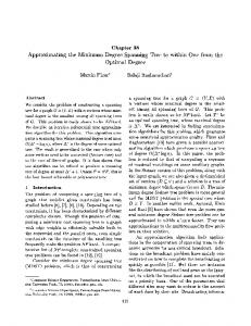
The maximum stretch of τ with respect to δ, denoted max-str(τ, δ), is defined accordingly. A partition of a set S is a collection P = {U1 , . . . , Uk }, where Ui ∩ Uj = ∅ for every S 1 ≤ i < j ≤ k and 1≤i≤k Ui = S. If S is the set of vertices of some graph, then the subsets U1 , . . . , Uk are called the clusters of the partition. For a partition P = {U1 , . . . , Uk } of V (G), S let E (P ) denote the set of edges internal to the clusters of P , i.e., E (P ) = Ui ∈P E (Ui ). Denote the set of edges external to P , namely, the edges connecting vertices in two different clusters, by E (P ) = E (G) \ E (P ). (Note that our definition does not require a cluster to be connected in G.) Every edge set F ⊆ E (P ) induces a logical cluster graph on P , obtained by contracting each cluster in P into a single node and replacing each edge (u, v) ∈ F , where u ∈ Ui and v ∈ Uj , by the edge (Ui , Uj ). We say that F induces a tree on P if the cluster graph induced by F on P is a tree. For a subset X ⊆ V (G), denote the set of clusters in P that intersect X by I(P, X) = {Ui ∈ P | Ui ∩ X 6= ∅}. Let H be a graph. In case that H is not necessarily connected, we denote the partition of V (H) that corresponds to the connected components of H by P (H). That is, two vertices x, y are in the same cluster in P (H) if and only if H admits a path between x and y. A central tool in our construction is a graph decomposition based on eliminating the edges of some ball of radius ρ. This decomposition is obtained as follows. For a metric δ over V (G), a vertex u ∈ V (G) and a positive integer ρ, erase from G the internal edges (but not the vertices) of the ball of radius ρ around u with respect to δ, E (Bδ (u, ρ)), and let G1 , . . . , Gr be the connected components remaining in G after erasing E (Bδ (u, ρ)). The collection {G(V (G1 )), . . . , G(V (Gr ))} is referred to as the (u, ρ, δ)-decomposition of G. Figure 1 illustrates the (u, 2, distG (·, ·))-decomposition of a graph G. We say that the vertex u is a ρ-center with respect to G and δ if |V (Gi )| ≤ n/2 for every 1 ≤ i ≤ r.
3
Lower bounds on the minimum max-stretch
In this section we establish some general lower bounds on the minimum max-stretch of a graph G. These lower bounds are used in Section 6 to yield the performance guarantee of our approximation algorithm. We begin with correlating the existence of a ρ-center with the minimum max-stretch of the graph. Theorem 3.1. Consider a graph G and a connected vertex induced subgraph H of G and let δ be the restriction of distG (·, ·) to the vertices of H. Then H admits a (2κ)-center with respect to δ, where κ = max-str(G).
4
2
G G1
G4 u
G7 ρ
6
G
5
G
G3
Figure 1: The decomposition of G with respect to distG (·, ·), u and ρ = 2. The dashed circle represents BdistG (·,·) (u, 2). Proof: Clearly, every spanning tree of G can be considered as a tree metric over V (G) that dominates the distances in G. In particular, there exists such a tree metric τ with max-str(τ, distG (·, ·)) = κ. In [Gupt01] it is proved that a tree metric τ over the vertices V can be transformed into a tree metric τ 0 over an arbitrary vertex subset U ⊆ V , such that τ (x, y) ≤ τ 0 (x, y) ≤ 8 τ (x, y) for every two vertices x, y in U . This result is improved in [HL02] for the special case where τ arises from the distances in an unweighted tree over the vertices V so that τ (x, y) ≤ τ 0 (x, y) ≤ 4 τ (x, y). It follows that there exists a tree metric δ T over V (H) that dominates δ such that max-str(δ T , δ) ≤ 4κ. We next show that this implies that H admits a (2κ)-center with respect to δ. Recall that in every n-vertex tree T , there exists a vertex u, named the centroid of T , whose removal disconnects T to subtrees of size at most n/2 each. Consider the tree T over V (H) that corresponds to δ T and let u be a centroid of T . (Observe that T is not necessarily a spanning tree of H.) Let T1 , . . . , Tk be the subtrees of T that result from the removal of u. Let {H 1 , . . . , H r } be the (u, 2κ, δ)-decomposition of H, namely, the connected components of H after erasing the internal edges of Bδ (u, 2κ). We claim that for every 1 ≤ i ≤ r, there exists some 1 ≤ j ≤ k such that V (H i ) ⊆ V (Tj ), hence u is a (2κ)-center of H and the theorem holds. Assume by way of contradiction that the claim is false and let H i be a subgraph of H that falsifies the claim, i.e., such that V (H i ) * V (Tj ) for any 1 ≤ j ≤ k. Since H i is connected, it follows that there exists an edge (x, y) ∈ E (H i ) such that x ∈ V (Tj ) and y ∈ V (Tj 0 ) for some 1 ≤ j < j 0 ≤ k. The edge (x, y) was not removed by the (u, 2κ, δ)decomposition of H, thus δ(u, x) ≥ 2κ and δ(u, y) ≥ 2κ, where at least one of these two 5
−
W1
−
x1 κ
F1
W2
x2 F2
+ W1
+
W2 H
¯ Figure 2: A κ-outspread subgraph H. The vertices x1 and x2 are connected in H. inequalities is strict. Therefore δ(u, x) + δ(u, y) > 4κ. Since δ T dominates δ, it follows that δ T (u, x) + δ T (u, y) > 4κ. But x and y are in different subtrees resulting from the removal of the centroid u from T , therefore δ T (x, y) = δ T (u, x) + δ T (u, y) > 4κ, in contradiction to the fact that max-str(δ T , δ) ≤ 4κ. The theorem follows. ¯ be Consider a graph G and let H be a connected vertex induced subgraph of G. Let H the subgraph induced on G by V (G) \ V (H). Denote the set of edges that cross between ¯ by F (H) = {(x, y) ∈ E (G) | x ∈ V (H) and y ∈ V (H)}. ¯ H and H Let W (H) be the set of endpoints of edges in F (H). We say that H is a κ-outspread subgraph of G if F (H) can be partitioned into two remote parts F1 and F2 with endpoints W1 and W2 , respectively, such that • distG (W1 , W2 ) ≥ κ and ¯ and x2 ∈ W2 ∩ V (H) ¯ such that H ¯ admits a • there exist two vertices x1 ∈ W1 ∩ V (H) simple path between x1 and x2 . ¯ is not necessarily connected but it is assumed to have some “connectivity” Note that H between endpoints of F1 and endpoints of F2 . In what follows, we define Wi+ = Wi ∩ V (H) ¯ for i = 1, 2. A κ-outspread subgraph is illustrated in Figure 2. and Wi− = Wi ∩ V (H) The existence of an outspread subgraph in a graph implies a lower bound on its minimum max-stretch, as established in the following theorem. Theorem 3.2. If a graph G admits a κ-outspread subgraph, then max-str(G) > κ. Proof: Consider a graph G and let H be a κ-outspread subgraph of G, with remote parts F1 and F2 with endpoints W1 and W2 . Let T be a spanning tree of G and suppose, towards deriving contradiction, that max-str(T ) ≤ κ. We begin by strengthening the second requirement of a κ-outspread subgraph, and prov6
¯ To show this, we ing that W1− and W2− are connected by a path fully contained in T ∩ H. prove that T contains a subtree T 0 such that • V (T 0 ) ∩ W1− 6= ∅, • V (T 0 ) ∩ W2− 6= ∅, ¯ and • T 0 lies entirely in H, • T 0 is maximal, namely, if T 00 is a subtree of T and V (T 0 ) ⊂ V (T 00 ), then V (T 00 ) ∩ V (H) 6= ∅. ¯ admits a simple By definition, since H is a κ-outspread subgraph of G, the subgraph H 0 path between W1− and W2− . Let ψ = (x01 , x11 , . . . , xs1 , xt2 , xt−1 2 , . . . , x2 ) be the shortest such − 1 ≤ s ≤ t ≤ len(ψ) . path, where x01 ∈ W1− , x02 ∈ W2− , κ ≤ len(ψ) = s + t + 1 and len(ψ) 2 2 j − − − Since ψ is a shortest path between W1 and W2 , it follows that distG (xi , Wi ) = j for i = 1, 2 and every vertex xji in ψ. By the definition of a κ-outspread subgraph, we have + distG (xji , Wi+ ) = j + 1 and distG (xji , W3−i ) ≥ min{κ + j + 1, s + t + 2 − j} for i = 1, 2 end j + every xi in ψ. Therefore distG (xs1 , Wi ) + distG (xt2 , Wi+ ) > κ for i = 1, 2. Consequently, The unique path between xs1 and xt2 in T does not contain any vertex in W1+ ∪ W2+ as otherwise, it is of length greater than κ, in contradiction to the assumption that max-str(T ) ≤ κ. + + Moreover, distG (xji , W3−i ) + distG (xj−1 , W3−i ) > κ for i = 1, 2 and every xji and xj−1 in ψ, i i j−1 j + hence the unique path between xi and xi in T does not contain any vertex in W3−i . Let πs,t be the unique path between xs1 and xt2 in T . As πs,t does not contain any vertex ¯ We would like to develop πs,t into a subtree T 0 as in W1+ ∪ W2+ , it must lie entirely in H. described above. For i = 1, 2, apply the following process to extend πs,t up to a vertex in Wi− without adding any edge of F (H). Initialize the variable subtree Υ to be the path πs,t . Initialize the variable integer j min by j min = min{j | xji ∈ V (Υ)} (j min is well defined as xs1 and xt2 are in Υ). If j min = 0, then we are done since the subtree Υ now contains a Wi− ¯ vertex and V (Υ) ⊆ V (H). min
Otherwise, apply a “developing step” as follows. Let χ be the unique path between xij min and xji −1 in T . The path χ does not contain any edge in F3−i since otherwise, it also + contains a vertex in W3−i . If χ contains an edge in Fi , then it must contain a vertex in Wi− right before that edge, in which case, the subtree Υ can be extended up to a vertex in Wi− without adding any F (H) edge and we are done. Otherwise, the path χ does not contain any F (H) edge at all, thus Υ can be extended so that j min decreases by a positive integral term without adding any edge in F (H). We repeat the “developing step” until j min = 0. Applying this process for i = 1, 2 yields a subtree T 0 of T such that T 0 contains a vertex in 7
¯ If T 0 is not W1− and a vertex in W2− and E (T 0 ) ∩ F (F ) = ∅, hence T 0 lies entirely in H. ¯ as long as possible. maximal, then extend it by adding adjacent edges of E (T ) ∩ E (H) We now turn to label the vertices of H by their location in T with respect to the subtree T . Pick an arbitrary vertex r ∈ V (T 0 ) and direct the edges of T towards r. Consider a vertex v in V (H) and let πv be the unique path from v to r in T . If u is the first vertex on πv such that u ∈ V (T 0 ), then we say that v is covered by u with respect to T 0 . Since T 0 is maximal, if v is covered by u, then the edge entering u on πv is in F and u must lie in Wi− for some i ∈ {1, 2}. For i = 1, 2, let 0
Ui = {v ∈ V (H) | v is covered by some vertex u ∈ Wi− with respect to T 0 } . Note that {U1 , U2 } is a partition of V (H). For two vertices x, y ∈ V (H), we say that x and y are separated by T 0 if x ∈ U1 and y ∈ U2 (or vice versa). Observe that this implies that the unique path between x and y in (the undirected) T contains an edge in F1 and an edge in F2 , thus its length is at least κ + 2. It follows that for an edge (x, y) in E (H), the vertices x and y cannot be separated by T 0 since otherwise, we have max-str(T ) > κ. But, by definition, the subgraph H is connected, therefore V (H) = Ui for some i ∈ {1, 2} and U3−i = ∅. Without loss of generality suppose that V (H) = U1 . Let y2− be a vertex in V (T 0 ) ∩ W2− and consider a neighbor y2+ ∈ W2+ of y in G. As y2+ is in U1 , it is covered by some vertex y1− ∈ W1− , hence distT (y2− , y2+ ) = distT (y2− , y1− ) + distT (y2+ , y1− ). Since distG (W1 , W2 ) ≥ κ, and since the distances in T dominate the distances in G, it follows that distT (y2− , y2+ ) ≥ 2κ, in contradiction to the assumption that max-str(T ) ≤ κ. The theorem follows.
4 4.1
The approximation algorithm Overview
b with max-str(G) b = κ, The main idea behind our algorithm is that given an n-vertex graph G b with the property that discarding there exists (as proved in Theorem 3.1) a vertex u ∈ V (G) the internal edges of the ball of radius 2κ around it decomposes the graph into several connected components, each of size at most n/2, with no edges crossing between them. Using this fact, our algorithm is invoked on the integer test values ρ ∈ (1, 2n], suspect of being 2κ. For every such test value, the algorithm tries to construct the output spanning tree Tb by looking for a vertex u and a decomposition as above, and merging a spanning tree Tlocal of the ball of radius 3ρ/2 around the vertex u (a superset of the ball of radius ρ), with the 8
spanning trees returned from the recursive calls made for every connected component of the decomposition. The ρ/2 gap between the radius of the ball used for decomposing the graph and the radius of the ball being spanned by the tree Tlocal ensures that the algorithm does not produce any cycle. This process is presented in more detail in the following subsections.
4.2
Algorithm Construct Tree
We present an algorithm named Algorithm Construct Tree, that given an n-vertex graph b and integral test value ρ, constructs a spanning tree Tb of G b with maximum stretch at G most 3ρ log n or reports failure. In Section 6 we prove that the algorithm does not fail if b Since the minimum max-stretch of G b is an integer in [1, n], a test value ρ ≥ 2max-str(G). b on which the algorithm does not fail can be guessed in O(log n) attempts, ρ ≤ 2max-str(G) to yield a 6 log n approximation algorithm. Throughout the execution of Algorithm Construct Tree, we maintain a forest (i.e., a b Initially, the forest cycle-free subgraph containing all the vertices) F of the input graph G. F is empty (does not contain any edge) and as the algorithm terminates, F contains the b Algorithm Construct Tree is recursive, where on each recursive spanning tree Tb of G. b as input and adds some invocation, the algorithm gets a vertex induced subgraph G of G edges of G to F. Upon termination of the recursive invocation on G, the vertices of V (G) all belong to a single tree in F (each connected component in F is a tree). Consider a recursive invocation of Algorithm Construct Tree on the vertex induced b Due to earlier recursive invocations, the forest F may already contain subgraph G of G. b that corresponds to the trees of F. some edges of G. Recall that P (F) is a partition of V (G) At the risk of abusing the notation, we shall use P (F) to denote the partition of V (G) that corresponds to connected components in F, i.e., each cluster in P (F) is a subset of V (G) and two vertices x, y ∈ V (G) are in the same cluster in P (F) if and only if F admits a path between x and y. To prevent the possibility of creating cycles in F, the algorithm will add an edge e ∈ E (G) to F only if e is external to P (F). Let P (F) = {U1 , . . . , Uk }. Note that the subgraph induced on G by the vertices in the cluster Ui is not necessarily connected, for each 1 ≤ i ≤ k. Let δ be the restriction of distGb (·, ·) to the vertices of G. Algorithm Construct Tree works as follows. It first finds a ρ-center u with respect to δ and identifies the set of clusters I(P (F), Bδ (u, 3ρ/2)), namely, the clusters of P (F) that intersect the ball of radius 3ρ/2 around u. If a ρ-center cannot be found, then the algorithm halts and reports “failure”. Next, a subset of the external edges of the partition P (F) that induces a tree (referred to as 9
the local tree Tlocal ) on these clusters is added to F. The edges internal to the ball of radius ρ around the vertex u (but not the vertices) are discarded from the graph and subsequently the graph decomposes into separate connected components1 . A recursive call is then made for each such connected component. The choice of the subset of edges that induces the local tree on the clusters I(P (F), Bδ (u, 3ρ/2)) is made by Procedure Construct Local Tree. Let F 0 be the forest F after the edges of the local tree were added to it. We say that the partition P (F 0 ) is a hub if P (F 0 ) contains at most one cluster U 0 (referred to later on as the kernel cluster ) that decomposes into several connected components of the graph decomposition and all other clusters remain intact, i.e., if for every cluster U in P (F 0 ) \ {U 0 }, there exists a connected component Gi of the graph decomposition such that U ⊆ V (Gi ). If P (F 0 ) is not a hub, then the algorithm halts and reports “failure”. If the algorithm manages to avoid the two failures, namely, it finds a ρ-center and P (F 0 ) is a hub, then we say that the current recursive invocation of the algorithm succeeds. Otherwise, we say that the current b with a larger recursive invocation fails, in this case the algorithm should be reinvoked on G test value ρ. A formal description of Algorithm Construct Tree is given in Table 1. Since the connected components G1 , . . . , Gr of the (u, ρ, δ)-decomposition of G are formed by discarding the edges internal to Bδ (u, ρ), we have the following. Observation 4.1. The vertex set Bδ (u, ρ) intersects Gi for every 1 ≤ i ≤ r.
4.3
Procedure Construct Local Tree
Consider a graph G. Let δ be a metric over V (G) and let P = {U1 , . . . , Uk } be a partition of V (G). We say that the graph C is the cliqued cluster graph of G with respect to P and δ if each cluster in P is completed into a clique, namely, • V (C) = V (G) and S • E (C) = E (P ) ∪ 1≤i≤k (Ui × Ui ). The graph C is weighted with edge lengths `(e) = δ(e) for every e ∈ E (C). Distances in a weighted graph are defined with respect to the length of the edges. The purpose of the following procedure, named Construct Local Tree, is to find a subset Tlocal of external edges from E (P (F)) that induces a tree on the clusters of 1
The connected components of this graph decomposition should not be confused with the clusters of the partition P (F).
10
b Input: A vertex induced subgraph G of G. Let δ be the restriction of distGb (·, ·) to the vertices V (G). 1. If |V (G)| = 1, then return. 2. Find a ρ-center u with respect to G and δ. If none exists, then halt and report “failure”. 3. Tlocal ← Construct Local Tree(G, u). 4. Set F ← F ∪ Tlocal . 5. Let G1 , . . . , Gr be the connected components of the graph remaining from G after discarding the edges of E (Bδ (u, ρ)). 6. If P (F) is not a hub (with respect to G1 , . . . , Gr ), then halt and report “failure”. 7. For every 1 ≤ i ≤ r, invoke Construct Tree(G(V (Gi ))). Table 1: Algorithm Construct Tree. I(P (F), Bδ (u, 3ρ/2)). Note that by the choice of Tlocal , it follows that P (F 0 ) \ P (F) contains a single cluster, named the kernel cluster U 0 , which is the union of all the clusters in P (F) that intersect Bδ (u, 3ρ/2). (See Figure 3.) The subset Tlocal should be chosen so that the diameter of the kernel cluster is not much greater than the sum of diameters of the P (F)-clusters it replaces (this requirement is presented formally and proved in Section 6). In principle, this task can be achieved by using a depth-(3ρ/2) shortest path tree rooted at u on the cliqued cluster graph C. However, a naive choice of such a shortest path tree might create cycles in the cluster graph induced on P (F). Procedure Construct Local Tree carefully avoids this complication. The procedure begins by constructing the cliqued cluster graph C of G with respect to P (F) and δ. Next, the vertex set U 0 is initiated to consist of the cluster of u in P (F) and the edge set Tlocal is initiated to be empty. The vertices of C are then processed in increasing order of distances from the vertex u. In Section 5 we prove that whenever Procedure Construct Local Tree is invoked, distC (·, ·) = δ, hence if the procedure processes the vertex x before it processes the vertex y, then δ(u, x) ≤ δ(u, y). Consider a vertex v when it is processed by the procedure and let Ui be v’s cluster in the partition P (F). If v ∈ / U 0 , then the procedure adds the vertices of Ui to U 0 and adds the edge (w, v) to Tlocal , where w is the predecessor of v in some shortest path from u to 11
T local 3 2
u
ρ
(a) Before
(b) After
Figure 3: The operation of Procedure Construct Local Tree. (a) The clusters of P (F) and the ball of radius 3ρ/2 around u. (b) Tlocal induces a tree on the clusters of I(P (F), Bδ (u, 3ρ/2)). The shaded area forms the kernel cluster U 0 . v. Note that (w, v) is an edge in E (G). This is reasoned by the fact that v must be the first vertex in Ui to be processed by the procedure (as otherwise, it was already in U 0 ), and since w was processed before v (as distC (u, w) < distC (u, v)). The procedure halts after all vertices at distance at most 3ρ/2 from u are processed and returns the edge set Tlocal . A formal description of Procedure Construct Local Tree is given in Table 2. Procedure Construct Local Tree can be implemented as a simple variant of the well known Dijkstra algorithm for finding shortest paths from a single source [Dijk59, CLR90]. Observation 4.2. The edge set Tlocal output by the procedure induces a tree on the clusters of I(P (F), U 0 ).
5
Correctness
In this section we prove that our algorithm generates a spanning tree of the given graph. In b and Tb stand for the unweighted n-vertex connected graph input to the first what follows, G invocation of Algorithm Construct Tree and the subgraph stored in F at the end of this invocation, respectively. For clarity of the argument, we assume that whenever Procedure Construct Local Tree adds an edge to Tlocal , this edge is being immediately added to F. This way the forest F is constructed gradually during the execution of the algorithm (rather
12
b and a vertex u ∈ V (G). Input: A subgraph induced graph G of G Output: An edge set Tlocal ⊆ E (P (F)) that induces a tree on the clusters of I(P (F), Bδ (u, 3ρ/2)). Let δ be the restriction of distGb (·, ·) to the vertices V (G). 1. Construct the cliqued cluster graph C of G with respect to P (F) and δ. 2. Let U be u’s cluster in P (F). 3. Set U 0 ← U and Tlocal ← ∅. 4. Let v1 , . . . , vn be the vertices of C in increasing order of distances from u, namely, v1 = u and distC (vi , u) ≤ distC (vj , u) for every 1 ≤ i < j ≤ n. 5. For i = 2, . . . , n, and as long as distC (vi , u) ≤
3ρ , 2
do:
(a) Let Ui be vi ’s cluster in P (F). (b) If vi ∈ / U 0 , then do: i. Set U 0 ← U 0 ∪ Ui . ii. Let π be a shortest path from u to vi in C. Let w be the predecessor of vi in π. iii. Set Tlocal ← Tlocal ∪ (w, vi ). 6. return Tlocal . Table 2: Procedure Construct Local Tree.
13
than instantly in line 4 of Algorithm Construct Tree). Consider an invocation of Algorithm Construct Tree on input G. Recall that F 0 denotes the forest F when Procedure Construct Local Tree returns (at the end of line 4 of Algorithm Construct Tree). Furthermore, recall that P (F) (respectively, P (F 0 )) denotes the partition of V (G) that corresponds to the connected components in F (resp., F 0 ) and that P (F 0 ) \ P (F) contains a single cluster U 0 , named the kernel cluster. Let G1 , . . . , Gr be the connected components of the graph decomposition (see line 5 of Algorithm Construct Tree). We shall use subscript l to denote recursion level l, i.e., let Gl , Ul0 and ul denote the input graph G, kernel cluster U 0 and center vertex u, respectively, in some invocation of the algorithm on recursion level l. Let Fl (respectively, Fl0 ) denote the forest F at the beginning (resp., at the end) of that execution of Algorithm Construct Tree on recursion level l. We begin by establishing a few fundamental facts regarding the execution of our algorithm. Lemma 5.1. Consider an invocation of Algorithm Construct Tree on input Gl on recursion level l and let x and y be two vertices in V (Gl ). Then we have the following. b such that len(π) > 1 and 1. If there exists a path π between x and y in the graph G V (π) ∩ V (Gl ) = {x, y}, then both x and y are in the same cluster in P (Fl ). 2. In the cliqued cluster graph C constructed Construct Local Tree, distC (x, y) = distGb (x, y).
in
line
1
of
Procedure
Proof: We prove the two claims simultaneously by induction on the recursion level l. On recursion level 0, we have the following. b are identical, hence such a path π does not exist and the first 1. The graphs G0 and G claim holds vacuously. b are identical and the second claim holds trivially. 2. The graphs C and G Now assume that the claims hold for every recursion level lower than l and consider an invocation of Algorithm Construct Tree on recursion level l. Let us first prove Claim 1. Consider a path π between the vertices x and y as in the claim. If all the internal vertices of the path π (namely, vertices other than the endpoints x and y) were already missing on the previous recursion level, i.e., V (π)∩V (Gl−1 ) = {x, y}, then due to the inductive assumption, x and y are in the same tree in Fl−1 , thus they are in the same tree in Fl and the claim holds. Otherwise, there must be some internal vertices of the path π that have existed in the 14
graph Gl−1 on the previous recursion level. We show that both x and y were in the kernel 0 0 cluster Ul−1 on the previous recursion level, thus they are in the same tree in Fl−1 and they remain in the same tree in Fl so that the claim holds. Let w be the internal vertex of π that still existed in Gl−1 which is closest to x in π, that is, the vertex w satisfies distπ (w, x) ≤ distπ (w0 , x) for every vertex w0 ∈ V (π)∩V (Gl−1 )\{x, y}. Let δ be the restriction of distGb (·, ·) to the vertices V (Gl−1 ) and let C be the cliqued cluster graph constructed in line 1 of Procedure Construct Local Tree when invoked on recursion level l − 1. We consider two cases (illustrated in Figure 4). b then since w does not exist in G, it follows that both (a) If (x, w) is an edge in E (G), w and x were in Bδ (ul−1 , ρ), hence distGb (ul−1 , x) = δ(ul−1 , x) ≤ ρ. By the inductive assumption on Claim 2, we have distC (ul−1 , x) = distGb (ul−1 , x). Therefore, since Procedure Construct Local Tree on recursion level l − 1 halted at distance 3ρ/2 from the center vertex ul−1 (see line 5 of Procedure Construct Local Tree), it follows that x is in the kernel 0 cluster Ul−1 . b then let Uw be w’s cluster in the partition P (Fl−1 ) on recursion level (b) If (x, w) ∈ / E (G), l−1. By the inductive assumption, the vertex x is in Uw as well (due to the subpath of π that starts at x and ends at w), thus w and x are in the same cluster in P (Fl−1 ) and they remain 0 in the same cluster U¯w in P (Fl−1 ). Since w is not a vertex in Gl , it follows that the cluster U¯w disintegrated into different connected components in the decomposition of the graph Gl−1 0 on the previous recursion level. Therefore the cluster U¯w must be the kernel cluster Ul−1 , since otherwise, the recursive invocation invocation of Algorithm Construct Tree on Gl−1 would have failed (see line 6 of the algorithm). 0 The same line of arguments shows that y ∈ Ul−1 as well, hence the claim holds. We now prove Claim 2. Consider the cliqued cluster graph C as in the claim. Let π be a b Some segments of the path π (namely, some shortest path between x and y in the graph G. consecutive sequences of vertices and edges between them) may be missing in the graph Gl on recursion level l. Consider such a missing segment and let x0 and y 0 be the vertices in π right before and right after this missing segment, respectively, that is, the path π consists of a segment between x and x0 , a segment between x0 and y 0 and a segment between y 0 and y, where the internal vertices of the segment between x0 and y 0 are all missing. By Claim 1, the vertices x0 and y 0 must be in the same tree in Fl (see Figure 5), hence they are in the same cluster in the partition P (Fl ) and by the definition of the cliqued cluster graph C, it follows that distC (x0 , y 0 ) = δ(x0 , y 0 ) = distGb (x0 , y 0 ). Therefore distC (x, y) = distGb (x, y) and the claim holds.
15
vertex not in Gl−1 x
w w ul−1
y
ρ
x
(a) (x,w) is an edge
y Uw
(b) (x,w) is not an edge
Figure 4: The two cases in the proof of Claim 1 of Lemma 5.1. In both cases, the vertex x 0 is in the kernel cluster Ul−1 .
vertex in Gl vertex not in Gl
y
x same tree
same tree
Figure 5: Proof of Claim 2 of Lemma 5.1. The path π contains some missing segments. By Claim 2 of the last lemma and since Procedure Construct Local Tree halts at distance 3ρ/2 from the source vertex u (see line 5 of Procedure Construct Local Tree), we have the following. Corollary 5.2. Upon termination of Procedure Construct Local Tree, the kernel cluster U 0 satisfies Bδ (u, ρ) ⊆ Bδ (u, 3ρ/2) ⊆ U 0 . Proposition 5.3. If l > 0, then for every cluster U in P (Fl ) there exists a cluster U¯ in 0 P (Fl−1 ) such that U ⊆ U¯ . Proof: By induction on the recursion level l. The claim holds vacuously for l = 0. Now assume that the claim holds for every recursion level lower than l and consider an invocation 16
of Algorithm Construct Tree on recursion level l. Suppose towards deriving contradiction 0 that there exists a cluster U ∈ P (Fl ) such that U * U¯ for any cluster U¯ in P (Fl−1 ). This implies that Fl contains a path π between some two vertices x, y ∈ U that are not 0 in the same cluster in P (Fl−1 ). Let π be such a path of minimum length. It follows that V (π) ∩ V (Gl ) = {x, y}, since otherwise, there exists some subpath of π with endpoints 0 x0 , y 0 ∈ U , where x0 and y 0 are in different clusters in P (Fl−1 ), in contradiction to π being the shortest such path. Recall that Gl is one connected component in the decomposition of the graph Gl−1 on 0 recursion level l − 1. The path π must contain some edges that did not exist in Fl−1 . Every such edge was added to F by a recursive invocation of Algorithm Construct Tree on some connected component H of the decomposition of Gl−1 , where V (H) ∩ V (Gl ) = ∅. Thus V (π) ∩ V (Gl−1 ) ' {x, y}, namely, the path π contains some vertices of Gl−1 other than x and y. Following the same line of arguments as in the proof of Claim 1 of Lemma 5.1, it can 0 be shown that x, y ∈ Ul−1 , in contradiction to the assumption that x and y are not in the 0 same cluster in P (Fl−1 ). The assertion follows. Next, we prove that the subgraph Tb output by the algorithm is indeed a spanning tree b of G. b Then at some stage during the execution Proposition 5.4. Consider an edge (x, y) ∈ E (G). of Algorithm Construct Tree, both x and y belong to Bδ (u, ρ) for the current ρ-center u. Proof: On every recursion level, either x, y ∈ Bδ (u, ρ) or there exists some connected component Gi (as in line 5 of the algorithm) such that x, y ∈ V (Gi ), in which case they stay together in the same connected component on the next recursion level. Let Tb be the forest F at the end of the execution of Algorithm Construct Tree on input b Since edges are added to F only if they are external to its corresponding partition graph G. P (F) (see Procedure Construct Local Tree), it follows that Tb is cycle-free. To see that Tb b By Proposition 5.4, at some stage during the is connected, consider an edge (x, y) ∈ E (G). execution of Algorithm Construct Tree, both x and y belong to Bδ (u, ρ) for the current ρ-center u. By Corollary 5.2, when Procedure Construct Local Tree terminates, the kernel cluster U 0 contains both x and y. Since every cluster in the partition P (F 0 ) corresponds to b is connected, we have the a tree in F 0 , the forest F 0 contains a path between x and y. As G following. Theorem 5.5. The graph Tb output by Algorithm Construct Tree is a spanning tree of the b input graph G.
17
6
Analysis
In this section we analyze the quality of the spanning tree generated by our algorithm. In Subsection 6.1 we prove that the recursive invocation of Algorithm Construct Tree on any b succeeds as long as the test value ρ is at least 2max-str(G). b vertex induced subgraph of G The approximation ratio guaranteed by our algorithm is then established in Subsection 6.2.
6.1
Successful recursive invocation
Consider an invocation of Algorithm Construct Tree on the vertex induced subgraph G of b with test value ρ ≥ 2max-str(G). b The proof that a rho-center can be found (see line 2 G of the algorithm) follows directly from Theorem 3.1. In order to prove that the partition P (F 0 ) is a hub (see line 6 of the algorithm), we have to show that the kernel cluster is the only cluster in P (F 0 ) that decomposes into several connected components of the graph decomposition. Let G1 , . . . , Gr be the connected components of the graph decomposition on this recursion level. Suppose towards deriving contradiction that there exists a cluster U in P (F 0 ) \ {U 0 } that decomposes into several connected components of the graph decomposition. (The execution of the algorithm halts at that stage.) Formally, let Xi = U ∩ V (Gi ), where without loss of generality Xi 6= ∅ for 1 ≤ i ≤ t and Xi = ∅ for t < i ≤ r, and suppose that t ≥ 2. Figure 6 illustrates a cluster U ∈ P (F) \ {U 0 } that decomposes into two connected components. Let δ be the restriction of distGb (·, ·) to the vertices of G. By the definition of the graph decomposition, every edge e in E (G) that crosses between V (Gi ) and V (Gj ), where 1 ≤ i < j ≤ r, satisfies e ∈ Bδ (u, ρ) × Bδ (u, ρ). Thus, by Observation 4.1 and Corollary 5.2, we have the following. Observation 6.1. The kernel cluster U 0 satisfies U 0 ∩ V (Gi ) 6= ∅ for every 1 ≤ i ≤ r. Furthermore, every edge e in E (G) that crosses between V (Gi ) and V (Gj ), where 1 ≤ i < j ≤ r, satisfies e ∈ U 0 × U 0 . Let τ be the tree in F that corresponds to the cluster U and let H be the subgraph b by V (τ ). We prove that H is a ρ/2-outspread subgraph of G b (refer to Section induced on G 3 for the definition of an outspread subgraph), in contradiction to Theorem 3.2. ¯ denote the subgraph induced on G b by the Following the notation of Section 3, let H b \ V (τ ). Let F (H) be be the set of edges in E (G) b that cross between H and vertices in V (G) ¯ and let W (H) be the set of endpoints of edges in F (H). Let F1 = {e ∈ F (H) | e ∈ E (G1 )}, H 18
G2 G1
U 111111111111111111 000000000000000000 000000000000000000 111111111111111111 U111111111111111111 000000000000000000 000000000000000000 111111111111111111 000000000000000000 111111111111111111 000000000000000000 111111111111111111 000000000000000000 111111111111111111 000000000000000000 111111111111111111 000000000000000000 111111111111111111 u 000000000000000000 111111111111111111 ρ 000000000000000000 111111111111111111 ’ U 000000000000000000 111111111111111111 000000000000000000 111111111111111111 000000000000000000 111111111111111111 000000000000000000 111111111111111111 000000000000000000 111111111111111111 000000000000000000 111111111111111111 000000000000000000 111111111111111111
Figure 6: The cluster U decomposes into the connected components G1 and G2 of the graph decomposition. namely, the edge set F1 consists of the edges that cross between U vertices and other vertices in the connected component G1 of the decomposition of G. Let F2 = F (H) \ F1 . By the choice of U and by Observation 6.1, the connected components G1 , . . . , Gt contain some vertices in U and some vertices not in U , thus F1 and F2 are non-empty. Let Wi be the endpoints of edges in Fi for i = 1, 2. Let Wi+ = Wi ∩ V (H) and let ¯ In order to prove that H is a ρ/2-outspread subgraph of G, b we have to Wi− = Wi ∩ V (H). b is large and to establish some connectivity show that the distance between W1 and W2 in G ¯ We start with the latter. properties of H and H. ¯ we have Clearly, the vertex induced subgraph H is connected (as τ is a tree in F). For H the following proposition. ¯ admits a Proposition 6.2. There exists two vertices x1 ∈ W1− and x2 ∈ W2− such that H simple path between x1 and x2 . Proof: Consider the subgraph G0 induced on G by V (G)\U . This subgraph is not necessarily connected, so let G00 be the connected component of G0 that contains the current ρ-center u (see Figure 6). By Observation 6.1, V (G00 ) ∩ V (Gj ) 6= ∅ for every 1 ≤ j ≤ t, therefore there exists a vertex xi in Wi− ∩ V (G00 ) for i = 1, 2. The proposition follows as G00 is a connected ¯ subgraph of H. We now turn to prove that distGb (W1 , W2 ) ≥ ρ/2. We begin by proving a general proposition on the behavior of our algorithm.
19
Proposition 6.3. Let x be a vertex in V (G) and let Ux be its cluster in the partition P (F). b such that y ∈ If there exists an edge (x, y) ∈ E (G) / V (G), then Bδ (x, ρ/2) ⊆ Ux . That is, b if x has a neighbor in G that does not appear in G, then each vertex w ∈ V (G) such that distGb (w, x) ≤ ρ/2 is in Ux . Proof: Let l be the last recursion level on which the vertices x and y coexisted in the graph, that is, in the decomposition of the graph Gl , the vertices x and y were separated into different connected components (l must be smaller than the current recursion level). As (x, y) is an edge, this could have happened only if both x and y were in Bδl (ul , ρ) on recursion level l, where δl is the restriction of distGb (·, ·) to the vertices V (Gl ). By Corollary 5.2, the kernel cluster Ul0 satisfies Bδl (ul , 3ρ/2) ⊆ Ul0 , thus w ∈ Ul0 for every vertex w ∈ V (Gl ) on recursion level l such that distGb (w, x) = δl (w, x) ≤ ρ/2. Therefore if such a vertex w still exists in the graph G, then it must lie in x’s tree in the current forest F, hence it is in Ux . Recall that the vertex set W1 consists of the endpoints of edges in F1 . Since every edge in F1 crosses between different clusters of the partition P (F), and since P (F) is a partition of the vertices in G, we have the following. b such that dist b (x, W1 ) ≤ ρ/2 is in V (G). Corollary 6.4. Every vertex x ∈ V (G) G Assume by way of contradiction that distGb (W1 , W2 ) < ρ/2. Let π be a shortest path in b between any vertex in W1 and any vertex in W2 . Since F is a cut, it follows that π lies G ¯ but it does not cross between them (as otherwise, π is not shortest). entirely in H or in H Since every vertex in π is at distance less than ρ/2 from W1 , it follows, by Corollary 6.4, that the path π lies entirely in the graph G. Since V (H) ∩ V (G) = U , and since there is no path connecting between W1+ and W2+ in G(U ), it follows that π connects between W1− and ¯ W2− in the subgraph induced by V (G) \ U on G (and in particular, in H). Recall that Algorithm Construct Tree uses the ball of radius ρ around the center u to decompose the graph (see line 5 of the algorithm), while the ball of radius (3ρ/2) is contained in the kernel cluster U 0 (see Corollary 5.2). Since every vertex in Wi− has a neighbor outside U 0 for i = 1, 2, it follows that distGb (Wi− , Bδ (u, ρ)) ≥ ρ/2. As len(π) < ρ/2, π cannot contain any edge internal to Bδ (u, ρ). But this implies that the endpoints of π should have been in the same connected component of the (u, ρ, δ)-decomposition of G, in contradiction to the fact that π has one endpoint in G1 and another in Gj for some 1 < j ≤ t. This establishes the following theorem. b and a test value ρ ≥ 2max-str(G), b Algorithm Theorem 6.5. Given an input graph G Construct Tree succeeds on each recursive invocation.
20
6.2
Approximation ratio
In this subsection we prove that if Algorithm Construct Tree succeeds on each recursive invocation when invoked with test value ρ, then the output spanning tree Tb satisfies b (recall that n is the number of vertices distTb (x, y) ≤ 3ρdlog ne for every edge (x, y) in E (G) b By Corollary 5.2 and Proposition 5.4, we know that at some stage of the input graph G). during the execution of the algorithm, the vertices x and y are both in the kernel cluster. Consequently we would like to bound the diameter of the kernel cluster in the output spanning tree Tb. In order to establish such a bound, we will actually prove a stronger claim, stating that the sum of the diameters of many clusters, the kernel cluster being one of them, is sufficiently small. For a collection of vertex subsets Λ = {U1 , . . . , Uk }, let X ϕ(Λ) = diamTb (Ui ) . 1≤i≤k
Recall that P (F) (respectively, P (F 0 )) stands for the partition of V (G) that corresponds to the trees of F at the beginning (resp., at the end) of the execution of Procedure Construct Local Tree. The kernel cluster U 0 is the sole cluster in P (F 0 ) \ P (F). Our subsequent analysis revolves on bounding the measure ϕ(·) for clusters I(P (F 0 ), V (Gi )), where Gi is a connected component of the graph decomposition (see line 5 of Algorithm Construct Tree). Proposition 6.6. Upon termination of Procedure Construct Local Tree, diamTb (U 0 ) ≤ 3ρ + ϕ(I(P (F), U 0 )) . Proof: The execution of Procedure Construct Local Tree halts at distance 3ρ/2 from the source vertex u (see line 5 of the procedure). Therefore the tree induced by Tlocal on the clusters of I(P (F), U 0 ) is of depth at most 3ρ/2 (when u is considered to be the root). Consider some two vertices x, y ∈ U 0 and let π be the unique path between x and y in Tb. The path π contains at most 2 · (3ρ/2) = 3ρ edges from the local tree Tlocal . Since π 0 = π − Tlocal , the rest of π, is a collection of segments internal to the P (F)-clusters replaced by U 0 , it follows that len(π 0 ) ≤ ϕ(I(P (F), U 0 )). Therefore len(π) ≤ 3ρ + ϕ(I(P (F), U 0 )) and the proposition holds. Assume without loss of generality that G1l−1 is the connected component of the decomposition of Gl−1 on recursion level l − 1 that corresponds to the graph Gl on recursion level � b V (G1 ) . Every cluster in P (F 0 ) \ {U 0 } l, that is, the graph Gl is identical to the graph G l−1 l l is also a cluster in P (F). By Proposition 5.3, and since every two vertices being connected 0 in Fl−1 remain connected in Fl0 , we have the following. 21
Corollary 6.7. For every cluster U ∈ P (Fl0 ) \ {Ul0 } there exists some cluster U¯ ∈ 0 I(P (Fl−1 ), V (G1l−1 )) such that U ⊆ U¯ and U¯ ∩ Ul0 = ∅. Lemma 6.8. On recursion level l of Algorithm Construct Tree, for every connected component Gi of the (u, ρ, δ)-decomposition generated in line 5 of the algorithm, ϕ(I(P (Fl0 ), V (Gi ))) ≤ 3ρ(l + 1) . Proof: By induction on l. On level 0, the only non-singleton cluster in the partition P (F00 ) is the kernel cluster U00 whose diameter in Tb is at most 3ρ. The diameter of a singleton cluster is 0. Therefore the sum of the diameters of all the clusters in P (F00 ) is at most 3ρ and the assertion holds. Now assume that the assertion holds for all levels lower than l and consider some connected component Gi of the graph decomposition on level l. By Corollary 0 6.7, for every cluster U ∈ P (Fl0 ) \ {Ul0 } there exists some cluster U¯ ∈ I(P (Fl−1 ), V (G1l−1 )) \ 0 I(P (Fl−1 ), Ul0 ) such that U ⊆ U¯ . In particular, for every cluster U ∈ I(P (Fl0 ), V (Gi )) \ {Ul0 } 0 0 there exists some cluster U¯ ∈ I(P (Fl−1 ), V (G1l−1 )) \ I(P (Fl−1 ), Ul0 ) such that U ⊆ U¯ . Since diamTb (U ) is monotone under set inclusion, i.e., U ⊆ U¯ implies diamTb (U ) ≤ diamTb (U¯ ), it follows that ϕ(I(P (Fl0 ), V (Gi ))) − diamTb (Ul0 ) = ϕ(I(P (Fl0 ), V (Gi )) \ {Ul0 })
(1)
0 0 ≤ ϕ(I(P (Fl−1 ), V (G1l−1 )) \ I(P (Fl−1 ), Ul0 )) 0 0 = ϕ(I(P (Fl−1 ), V (G1l−1 ))) − ϕ(I(P (Fl−1 ), Ul0 )) ,
(2)
where Equality (1) holds since the kernel cluster must intersect every connected component of the graph decomposition (by Observation 4.1 and Corollary 5.2) and Equality (2) holds since Ul0 ⊆ V (G1l−1 ). Thus 0 0 ϕ(I(P (Fl0 ), V (Gi ))) ≤ diamTb (Ul0 ) + ϕ(I(P (Fl−1 ), V (G1l−1 ))) − ϕ(I(P (Fl−1 ), Ul0 )) . 0 By Proposition 5.3, every cluster in P (Fl ) is a subset of some cluster in P (Fl−1 ), hence 0 ϕ(I(P (Fl ), Ul0 )) ≤ ϕ(I(P (Fl−1 ), Ul0 )) ,
and consequently 0 ϕ(I(P (Fl0 ), V (Gi ))) ≤ diamTb (Ul0 ) − ϕ(I(P (Fl ), Ul0 )) + ϕ(I(P (Fl−1 ), V (G1l−1 ))) .
By Substituting the inequality of Proposition 6.6, we get 0 ), V (G1l−1 ))) . ϕ(I(P (Fl0 ), V (Gi ))) ≤ 3ρ + ϕ(I(P (Fl−1
22
0 The inductive assumption implies that ϕ(I(P (Fl−1 ), V (G1l−1 ))) ≤ 3ρl, thus
ϕ(I(P (Fl0 ), V (Gi ))) ≤ 3ρ + 3ρl = 3ρ(l + 1) . The assertion follows. b By Proposition 5.4, at some stage during the Let (x, y) be an arbitrary edge in E (G). execution of Algorithm Construct Tree we get x, y ∈ Bδ (u, ρ) for the current ρ-center u. Let the recursion level of this stage be l and let δ be the restriction of distGb (·, ·) to the vertices V (Gl ). Since x, y ∈ Bδ (ul , ρ), it follows, due to Corollary 5.2, that x, y ∈ Ul0 . Let Gi be any connected component of the (ul , ρ, δ)-decomposition on this level. By Observation 4.1 and Corollary 5.2 we have V (Gi ) ∩ Ul0 6= ∅, hence Ul0 ∈ I(P (Fl0 ), V (Gi )). It follows that distTb (x, y) ≤ diamTb (Ul0 ) ≤ ϕ(I(P (Fl0 ), V (Gi ))) . By Lemma 6.8, and since the depth of the recursion is at most dlog ne (as the size of each graph input to the recursive algorithm decreases by a factor of at least 2), ϕ(I(P (Fl0 ), V (Gi ))) ≤ 3ρ(l + 1) ≤ 3ρ dlog ne . Therefore distTb (x, y) ≤ 3ρdlog ne. As the maximum stretch of a spanning tree is always obtained on a pair of vertices that form an edge in the original graph [CC95], Theorems 5.5 and 6.5 imply the following. b Algorithm Construct Tree can be invoked with Theorem 6.9. Given an n-vertex graph G, b satisfying max-str(Tb) = O(log n) different test values to generate a spanning tree Tb of G b O(log n) · max-str(G).
7
Tightness of the analysis
In this section we prove that the analysis presented in Section 6 is tight. Recall that our approximation algorithm invokes Algorithm Construct Tree with different test values ρ ∈ (1, 2n], finally returning the output of a successful invocation with the smallest ρ. For the sake of the analysis in this section, we assume that the approximation algorithm ignores the spanning trees output by successful invocations with higher test values, although some of these spanning trees may admit smaller maximum stretch. Lemma 7.1. For every integer d ≥ 1 there exists an unweighted graph Gd with n(d) = Θ(2d ) vertices such that max-str(Gd ) is constant while Algorithm Construct Tree, when invoked on Gd with test value ρ = 2, constructs a spanning tree with maximum stretch Ω(log n). 23
r
r’
edges of T edges of T’ bridge edges
Figure 7: Gd for d = 4. Proof: Given an integer d ≥ 1, construct the unweighted graph Gd as follows. Let T and T 0 be two complete binary trees of depth d, with roots r and r0 , respectively. Connect the two trees to each other by adding a bridge edge between every pair of corresponding vertices. Split every edge (x, y) in T by adding a new vertex z and replacing (x, y) with new edges (x, z) and (y, z). Figure 7 illustrates the construction of G4 . Since the number of vertices in a depth d complete binary tree is 2d+1 − 1 and since the number of new vertices added to T is 2d+1 − 2 (equals to the number of edges in a depth d complete binary tree), it follows that n(d) = |V (Gd )| = 2 (2d+1 − 1) + 2d+1 − 2 = 6 · 2d − 4 . It is easy to verify that the spanning tree obtained by removing the edges of T 0 and remaining with the edges of T plus the bridge edges has maximum stretch 4. On the other hand, when Algorithm Construct Tree is invoked on Gd with test value ρ = 2, if the “original” vertices of T (the ones that existed in T before splitting the edges) are chosen to be the 2-centers on each recursive invocation, then the spanning tree Tb returned by the algorithm looks like the union of T and T 0 with their roots connected by an edge, i.e., E (Tb) = E (T )∪E (T 0 )∪{(r, r0 )}. Let l be an arbitrary leaf in T and let l0 be its corresponding leaf in T 0 . The unique path between l and l0 in Tb goes via the edge (r, r0 ) and it is of length 2d + 1 + d = 3d + 1. Therefore Tb has maximum stretch Ω(d) = Ω(log (n(d))).
24
8
Hardness of approximation
As mentioned in Subsection 1.2, it is NP-hard to decide, for an arbitrary unweighted graph G, whether or not max-str(G) ≤ 4 [CC95]. Moreover, since the maximum stretch of a tree on an unweighted graph is always obtained on a pair of vertices that form an edge in the original graph, it follows that max-str(G) must be an integer. Therefore we have the following. Corollary 8.1. It is NP-hard to approximate the MMST problem on unweighted graphs by a ratio better than 5/4. We show that unless P = NP, the problem cannot be approximated additively by a factor of o(n). Lemma 8.2. It is NP-hard to distinguish between unweighted graphs with minimum maxstretch at most 5k − 1 and those with minimum max-stretch at least 6k − 1 for any positive integer k. Proof: By reduction from the problem of deciding whether an arbitrary unweighted graph has minimum max-stretch at most 4. Consider some positive integer k. Given an arbitrary unweighted graph G, construct the unweighted graph G0k by replacing every edge (u, v) ∈ E (G) with a unique path Pu,v of length k between u and v. Observe that every spanning tree T 0 of G0k corresponds to a spanning tree T of G where the edge (u, v) is in E (T ) if and only if all the edges of Pu,v are in E (T 0 ). Moreover, if the spanning tree T 0 of G0k corresponds to the spanning tree T of G then since T 0 is connected, it follows that ( k, if (u, v) ∈ E (T ), |E (T 0 ) ∩ E (Pu,v )| = k − 1, otherwise for every (u, v) ∈ E (G), i.e., the tree T 0 is missing at most a single edge from every such path Pu,v . Therefore max-str(T 0 , G0k ) = k · (max-str(T, G) + 1) − 1. Thus if G has minimum max-stretch at most 4, then G0k has minimum max-stretch at most 5k − 1. Otherwise, if G has minimum max-stretch at least 5, then G0k has minimum max-stretch at least 6k − 1. Given an approximation algorithm A for the MMST problem on unweighted graphs and an unweighted graph G, let A(G) denote the tree returned by A when invoked on G. Corollary 8.3. If there exist some real δ = o(n) and � > 0 and an approximation algorithm A for the MMST problem on unweighted graphs with performance guarantee max-str(A(G), G) ≤ δ + (6/5 − �) · max-str(G) for every unweighted graph G, then P = NP.
25
References [AKPW95] N. Alon, R. M. Karp, D. Peleg and D. West. A graph theoretic game and its application to the k-server problem. SIAM. J. Comput. 24: 78–100, 1995. [ADDJ+93] I. Alth¨offer, G. Das, D. Dobkin, D. Joseph and J. Soares. On sparse spanners of weighted graphs. Discrete and Computational Geometry, 9:81–100, 1993. [Bart98]
Y. Bartal. On approximating arbitrary metrics by tree metrics. In Proc. 30th ACM Symp. on Theory of Computing, 1998.
[Cai94]
L. Cai. NP-completeness of minimum spanner problems. Discrete Applied Mathematics, 48:187–194, 1994.
[CC95]
L. Cai and D. Corneil. Tree spanners. SIAM J. on Discrete Mathematics, 8:359– 387, 1995.
[CLR90]
T. H. Cormen, C. E. Leiserson and R. L. Rivest. Introduction to Algorithms. The MIT Press, 1990.
[Dijk59]
E. W. Dijkstre. A note on two problems in connexion with graphs. Numerische Mathematik, 1:269–271, 1959.
[DHZ96]
D. Dor, S. Halperin and U. Zwick. All pairs almost shortest paths. In Proc. 37th IEEE Symp. on Foundations of Computer Science, pages 452–461, 1996.
[EEST05] M. Elkin, Y. Emek, D. A. Spielman and S. -H. Teng. Lower-stretch spanning trees. In Proc. of the 37th Annual ACM Symposium on Theory of Computing, pages 494–503, 2005. [FK98]
S. P. Fekete and J. Kremer. Tree spanners in planar graphs. In Proc. 24th Int. Workshop on Graph Theoretic Concepts in Computer Science. Springer-Verlag, 1998.
[FRT03]
J. Fakcharoenphol, S. Rao and K. Talwar. A tight bound on approximating arbitrary metrics by tree metrics. In Proc. of the 35th Annual ACM Symposium on Theory of Computing, pages 448–455, 2003.
[Gupt01] A. Gupta. Steiner points in tree metrics don’t (really) help. In Proc. 12th ACMSIAM Symp. on Discrete Algorithms, pages 220–227, 2001.
[HL02]
R. Hassin and A. Levin. Minimum restricted diameter spanning trees. In Proc. 5th Int. Workshop on Approximation Algorithms for Combinatorial Optimization. Springer-Verlag, 2002.
[PR99]
D. Peleg and E. Reshef. A variant of the arrow distributed directory protocol with low average-case complexity. In Proc. 26th Int. Colloq. on Automata, Languages & Prog., pages 615–624, 1999.
[PS89]
D. Peleg and A. A. Sch¨affer. Graph spanners. J. of Graph Theory, 13:99–116, 1989.
[PT01]
D. Peleg and D. Tendler. Low stretch spanning trees for planar graphs. Technical Report MCS01-14, The Weizmann Institute of Science, 2001.
[PU89]
D. Peleg and J. D. Ullman. An optimal synchronizer for the hypercube. SIAM J. on Computing, 18(2):740–747, 1989.