Approximating Multi-objective Hyper-heuristics for Solving 2D ... - Core

Approximating Multi-objective Hyper-heuristics for Solving 2D Irregular Cutting Stock Problems Juan Carlos Gomez and Hugo Terashima-Mar´ın Tecnol´ ogico de Monterrey Monterrey, Nuevo Le´ on 64849, M´exico [email protected], [email protected]

Abstract. This article presents a method based on the multi-objective evolutionary algorithm NSGA-II to approximate hyper-heuristics for solving irregular 2D cutting stock problems under multiple objectives. In this case, additionally to the traditional objective of minimizing the number of sheets used to fit a finite number of irregular pieces, the time required to perform the placement task is also minimized, leading to a bi-objective minimization problem with a tradeoff between the number of sheets and the time required for placing all pieces. We solve this problem using multi-objective hyper-heuristics (MOHHs), whose main idea consists of finding a set of simple heuristics which can be combined to find a general solution for a wide range of problems, where a single heuristic is applied depending on the current condition of the problem, instead of applying a unique single heuristic during the whole placement process. The MOHHs are approximated after going through a learning process by mean of the NSGA-II, which evolves combinations of condition-action rules producing at the end a set of Pareto-optimal MOHHs. We tested the approximated MMOHHs on several sets of benchmark problems, having outstanding results for most of the cases.

Keywords: Hiper-Heuristics; Multi-Objective Optimization; Cutting; Evolutionary Computation

1

Introduction

Bin packing and cutting stock problems are well-known classical problems with many applications in different areas like operational research, logistics, engineering and related subjects. The basic idea and main goal consists of fitting a finite number of pieces into a minimum number of bins, subject to a practical set of restrictions and requirements. For small combinatorial problems, exact methods like linear programming can be applied. However, when larger and more complex problems appear, exact solutions are not a reasonable choice since the search space grows exponentially, and so does the time to find the optimal solution. Various heuristic and approximate approaches that guarantee finding near optimal solutions have been proposed [11]. However, no reliable method that can

solve a large variation of instances of a given problem has been found. In general, methods work well for a few instances, but are deficient for many others. A hyper-heuristic is a method used to define a high-level heuristic that controls low-level heuristics [1]. The hyper-heuristic decides when and where to apply each single low-level heuristic, depending on the given problem state and the search space. In recent work, based on the research by Ross et al. [13], evolutionary approaches have been used to generate hyper-heuristics for the 2D regular and irregular cutting stock problems [15][16]. These methods assemble a combination of single heuristics (each concerned with selection and placement of a piece), and this combination takes into account the quality of partial solutions provided by the single heuristics. Nevertheless, the majority of the works devoted to the problems of bin packing and cutting stocks are focused on mono-objective solutions like minimizing the trim loss; however these problems are naturally multi-objective, since several (opposite) objectives can be optimized at the same time. Just recently some works devoted to multi-objective cutting and packing problems have started to emerge like [7][12]; the present article intends to contribute with another perspective of solution for these problems. In this work we are focused on problems involving cutting 2D irregular pieces where two objectives need to be minimized: the number of sheets used to cut a finite number of pieces with irregular shapes and the time required to perform the placement of all the pieces inside the sheet. The aim of this paper is to present a method based on the Multi-Objective Evolutionary Algorithm (MOEA) [3] NSGA-II [4] to approximate generalized Multi-Objective Hyper-Heuristics (MOHH) in order to solve the cutting-stock problem describe above. We use NSGA-II with a variable-length representation. This algorithm evolves combinations of condition-action rules through a learning process, producing at the end a set of Pareto-optimal MOHHs. Finally, we test the approximated MOHHs on several sets of benchmark problems. Results of the proposed model in the 2D cutting-stock problem are truly encouraging. The remainder of this paper is organized as follows. Section 2 describes the multi-objective cutting-stock problem. Section 3 presents the proposed solution based on MOHH. This is followed by the experimental setup, the results and discussion in section 4. Finally, in section 5 we include our conclusions and some ideas for future work.

2

Description of the Problem

The Cutting-Stock and Packing Problems (CuSPPs) are among the earliest problems in the literature of operational research. In 1939, Kantorovich [10] studied applications in all the industries whose products were in a flat sheet form. An extensive literature on the CuSPPs and their applications has developed since. For example, Golden in [8] gives an abstract description of a variety of different solution methods; in [2] Chen et al. discuss a number of solution methods, and Dyckhoff in [5] lists a number of solution methods and applications and presents a systematic categorization of cutting and packing problems.

Here we solve instances of problems considered as Single Bin-Size 2D CuttingStock Problems with Irregular Shape Pieces. We can define formally these problems as: given a set L = (a1 , a2 , ...an ) of pieces to be cut, each one of size s(ai ) ∈ (0, Ao ], from a set m of cutting stock sheets of size Ao , the multi-objective goal of cutting the pieces from the sheets can then be modeled as follows. minimize z1 = minimize z2 = s.t.

Pn i=1

m X i=1 n X

yi

(1)

ti

(2)

i=1

s(ai ) ≤ mAo

where expression 1 minimizes the number yi of needed sheets, and expression 2 minimizes the time to place all the pieces inside the sheets, where ti indicates the required time to put the piece ai inside a sheet, using a given heuristic. Intuitively, the two objective functions are of conflicting nature. While a large number of sheets allows the placement of all the pieces very fast, having z2 → 0, the trim of material will be also large; on the other hand, a solution with z1 → 0, will tend to require more time to place all the pieces in the best position in order to do not waste material. This means that not a single solution x exists in the set of feasible solutions X that equally minimizes both objective functions z1 and z2 . Then, we have a vector optimization problem in which a solution x ∈ X is evaluated with respect to a vector Z(x) = (z1 (x), z2 (x)). The solution of the problem has consequently to be seen in the identification of all efficient outcomes or the Pareto-set P , defined as follows: Definition 1. (Dominance): Z(x) is said to dominate Z(x0 ) iff zk (x) ≤ zk (x0 ) ∀k = 1, . . . , K ∧ ∃k|zk (x) < zk (x0 ). We denote the dominance of Z(x) over Z(x0 ) with Z(x) ¹ Z(x0 ). Definition 2. (Efficiency, Pareto-optimality): The vector Z(x), x ∈ X is said to be efficient iff ¬∃Z(x0 ), x0 ∈ X|Z(x0 ) ¹ Z(x). The corresponding alternative x is called Pareto-optimal and the set of all Pareto-optimal alternatives is the Pareto-set P .

3

Multi-Objective Hyper-Heuristics Solution Approach

Hyper-heuristics deal with the process of choosing good single heuristics for solving the problem at hand. The idea is to discover a combination of single heuristics that can perform well on a whole range of problems and in such a way that one heuristic’s strengths make up for the drawbacks of another [14]. The rationale is that there is no a unique best single heuristic to solve well all the instances of a problem, since certain problems may contain features that would enable a specific heuristic to work well, but those features may not be present in other problems. Then, a combination of heuristics, selectively applied based on the features present in a problem, may work well on a wide range of problems.

3.1

Single Heuristics

For the 2D irregular cutting-stock problem, the related single heuristics must define the exact location of the pieces inside the sheet. In this work two kinds of single heuristics to be combined by the Multi-Objective Hyper-Heuristics (MOHHs) were considered: one kind for selecting the pieces and sheets, and the other for placing the pieces into the sheets. The selection heuristics are shown below. Some of these heuristics are described in more detail in [13] and [9]. - First Fit (FF).- Consider the opened sheets in turn in a fixed order and place the piece in the first one it fits. - First Fit Decreasing(FFD).- Sort pieces in decreasing order, and the largest one is placed according to FF. - First Fit Increasing (FFI).- Sort pieces in increasing order, and the smallest one is placed according to FF. - Filler + FFD.- Places as many pieces as possible within the open sheets. If at least one piece has been placed, the algorithm stops. The FFD algorithm is applied, otherwise. - Next Fit (NF).- Use the current sheet to place the next piece, otherwise open a new one and place the piece there. - Next Fit Decreasing (NFD).- Sort the pieces in decreasing order, and the largest one is placed according to NF. - Best Fit (BF).- This places the piece in the opened sheet where it best fits (i.e. with the minimum waste). - Best Fit Decreasing (BFD).- Same as the previous one, but sorting the pieces in decreasing order. - Worst Fit (WF).- It places the piece in the opened sheet where it worst fits (i.e. with the largest waste). - Djang and Fitch (DJD).- It places pieces in a sheet, taking pieces by decreasing size until the sheet is at least one-third full. Then, it initializes w, a variable indicating the allowed waste, and looks for combinations of 1,. . .,5 pieces producing a waste w. If any combination fails, it increases w accordingly. The placement heuristics, described in detail in [17], are the following: - Bottom-Left (BLI).- The piece starts at the top right corner of the sheet and it slides down and left with a sequence of movements until no other movement is possible. If the final position does not overlap the sheet boundaries, the piece is placed in that position. The heuristic does not allow a piece to skip around another placed piece. It’s a simple and fast heuristic. - Constructive Approach (CA).- The heuristic starts by placing the first piece at the bottom and left of the sheet. Then, the next piece is placed in one of the five positions: (x, 0), (0, y), (x, y), (x, y)and (x, y), where x, x, y, and y are the maximum and minimum coordinates in x and y in relation to the first piece. For each position, the next piece slides following down and left movements, and the one that places the piece deepest (bottom and left) is chosen, except in special

cases such as when a hole is formed. - Constructive-Approach (Minimum Area) (CAA).- In this modification of the previous heuristic, the best position from the list is selected based on which one yields the bounding rectangle with minimum area, containing all pieces, and that fits in the bottom left corner of the object. - Constructive-Approach (Maximum Adjacency) (CAD).- With the first piece only the four corners of the sheet are considered. For the subsequent pieces, the possible points are the same than in CA. For each position in the list the piece starts in that position and its adjacency (i.e. the common boundary between its perimeter and the placed pieces and the sheet edges) is computed. Then, the piece is slid down and left and the adjacency is computed again. The position with the largest adjacency is selected as the position of the new piece. 3.2

NSGA-II

In this paper we use the NSGA-II [4], a MOEA [3] with variable length chromosomes as the approach to approximate generalized MOHHs to solve the cuttingstock problem as described above. The NSGA-II (Elitist Non-Dominated Sorting Genetic Algorithm) is a well known and with good behavior MOEA proposed by Deb et al. in [4], used as a reference for many works in multi-objective optimization. In this algorithm, initially a random parent population P0 of size N is created. The population is sorted based on the non-domination. Each solution is assigned a fitness (or rank) equal to its non-domination level (1 is the best level, 2 is the next-best level, and so on). Thus, minimization of this rank is assumed. The normal binary tournament selection, recombination, and mutation operators are used to create an offspring population Q0 of size N . After that, a combined population Rt = Pt +Qt is formed. Next, the population Rt is sorted according to non-domination, forming the fronts F = F1 , F2 , . . .. Since all previous and current population members are included in Rt , elitism is ensured. Now, solutions belonging to the best non-dominated set F1 are of best solutions in the combined population and must be emphasized more than any other solution inside it. If the size of F1 is smaller than N , all the members of the set F1 are chosen for the new population Pt+1 . The remaining members of the population Pt+1 are chosen from subsequent non-dominated fronts in the order of their ranking. Thus, solutions from the set F2 are chosen next, followed by solutions from the set F3 , and so on. This procedure is continued until no more sets can be accommodated. The new population Pt+1 is now used for selection, crossover, and mutation to create a new population Qt+1 , and the process is repeated until a stop criteria is satisfied. 3.3

Model

In this work we adapted the evolutionary model proposed in [17], which produces general hyper-heuristics using a simplified representation of the state of the problem. A chromosome in the NSGA-II algorithm inside our model consists of a number of points in this simplified state space, each point being labeled with a

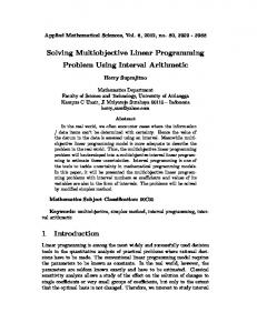
Fig. 1. Graphical representation of a chromosome using the simplified state space

given heuristic. Then, if we have a problem state S in the simplified state space, we find the nearest point in the chromosome and apply the heuristic recorded on the points label. This will transform the problem to a new state S 0 , and the process is repeated until a complete solution has been constructed. A chromosome therefore represents a complete recipe for solving a problem, using this simple algorithm: until the problem is solved, (a) determine the current problem state S, (b) find the nearest point to it, (c) apply the heuristic attached to the point, and (d) update the state. The NSGA-IIs task is to find a set P of Pareto-optimal chromosomes that are capable of obtaining good solutions for a wider variety of problems, taking in consideration the trade off between the two minimization objectives defined in equations 1 and 2; the set of chromosomes P are the multi-objective hyper-heuristics we are seeking. Representation.- Each chromosome is composed by a variable number of blocks. The initial number of blocks is randomly created and after it, the evolutionary process can create or delete blocks. Each block includes nine numbers. The first eight lie in the range 0 to 1 and represent the problem state, so a block can be seen as the labeled point. The label is the ninth number, which identifies a particular action (single heuristic). The NSGA-II’s task is to create and evolve a certain number of such labeled points, using the problem-solving algorithm defined above, where to determine the nearest point we use Euclidean distance. In the problem state, the first three numbers are related to rectangularity, a quantity that represents the proportion between the area of a piece and the area of a horizontal rectangle containing it. These numbers represent the fraction of remaining pieces with high rectangularity [0.9,1], medium rectangularity [0.5,0.9] and low rectangularity [0,0.5]. The fourth to seventh numbers are related to the area of pieces, and are categorized as follows (Ao is the sheet area, Ap is the piece area): huge (Ao /2 < Ap ); large (Ao /3 < Ap ≤ Ao /2); medium (Ao /4 < Ap ≤ Ao /3); and small (Ap ≤ Ao /4). The eighth number represents the fraction of the total number of pieces that remain to be placed. The label is selected from all possible combinations of selection and placement heuristics. Figure 1 shows a graphical representation of a chromosome using the simplified state space. This simplified feature space intends to represent the essential information about the geometry (rectangularity), and occupied and free space of the problem’s

whole configuration in a given step of the solution process. More features can be added or considered but with the corresponding increase in complexity. The current problem’s state is compute in each step of the solution process, taking the information stored in the model about the pieces assigned, pieces free and open (available) sheets. Finally, there are 40 different combinations for the action as shown in Table 1. Action 1 2 3 4 5 6 7 8 9 10 11 12 13 14 15 16 17 18 19 20

Selection

Placement

BLI - Bottom Left CA - Constructive CAA - Constructive-M. CAD - Constructive-M. FFD BLI - Bottom Left CA - Constructive CAA - Constructive-M. CAD - Constructive-M. FFI BLI - Bottom Left CA - Constructive CAA - Constructive-M. CAD - Constructive-M. Filler+FFD BLI - Bottom Left CA - Constructive CAA - Constructive-M. CAD - Constructive-M. NF BLI - Bottom Left CA - Constructive CAA - Constructive-M. CAD - Constructive-M.

Action Selection

FF

21 22 23 24 25 26 27 28 29 30 31 32 33 34 35 36 37 38 39 40

Area Adjacency

Area Adjacency

Area Adjacency

Area Adjacency

Area Adjacency

NFD

BF

BFD

WF

DJD

Placement BLI - Bottom Left CA - Constructive CAA - Constructive-M. CAD - Constructive-M. BLI - Bottom Left CA - Constructive CAA - Constructive-M. CAD - Constructive-M. BLI - Bottom Left CA - Constructive CAA - Constructive-M. CAD - Constructive-M. BLI - Bottom Left CA - Constructive CAA - Constructive-M. CAD - Constructive-M. BLI - Bottom Left CA - Constructive CAA - Constructive-M. CAD - Constructive-M.

Area Adjacency

Area Adjacency

Area Adjacency

Area Adjacency

Area Adjacency

Table 1. List of possible actions.

The Fitness Functions.- Each MOHH is evaluated using two fitness functions, one for the waste of space in the sheet and another for the total time needed to place the pieces on the sheet. The waste of space in a given sheet and the corresponding fitness function are defined as: Pk i=1

W =1−

s(ai )

A Pm o

F F1 =

i=1

Wi2

m

(3) (4)

where k is the number of pieces inside the sheet, s(ai ) the size of each piece, Ao the size of the sheet and m is the number of sheets used. The second fitness function is defined as: F F2 =

n X

t(h(ai ))

(5)

i=1

where t(h(ai )) is the required time to place the piece ai using the heuristic h. During the NSGA-II process, when a new individual (MOHH) is created (in the first parent population or in the subsequent children populations), a set of 5 problems is assigned to it. These problems are selected randomly from the training set. Then, the individual is evaluated with each problem using the

previous fitness functions, the fitness values are added and averaged to obtain two final fitness values: P5

F Fj (pi ) ; j = 1, 2 (6) 5 where pi is the i-th problem assigned to the individual and index j indicates the number of fitness function. During the evolution, if an individual from the parent population survives for the next generation, a new problem is assigned to it and the fitness functions are recomputed. F F Tj (M OHH) =

F F Tjl (M OHH)

i=1

(F F Tjl−1 ∗ np ) + F Fj (p) = ; j = 1, 2 np + 1

(7)

where F F Tjl is the value of the j-th total fitness function for the generation l, np is the number of problems the individual has solved until now and F Fj (p) is the value of the j-th fitness function for the new problem. This task of assign new problems to old individuals and recompute their fitness values continue during the whole evolutionary process. Genetic Operators.- In this work we use two uniform versions of crossover and mutation, the first version works at the block level and the second one works with the internal elements of each block. In the block level cross-over a random number of complete blocks is exchanged between two parent individuals to create two children individuals; since the number of blocks in each chromosome (individual) is variable, the random number is less or equal to the shortest chromosome. In the block level mutation, given certain probability, a randomly selected block can be deleted from the chromosome or a randomly created block can be added to the chromosome. In the internal level cross-over and mutation, they select a random number of blocks and for each block a random number of values to be interchanged or mutate, depending on the operator.

4 4.1

Experimental Results Problem Instances

For this work we generated 18 different types of problems, with 30 instances for each type, totalling 540 instances. Their characteristics can be seen in Table 2. We also added a problem from the literature [6], which was scaled by a factor of 10 in order to have the sheet size of 300 × 300. Instances of type G are the only problems with unknown optimal number of objects, since they were produced after alterations to randomly generated problems with known optimum. 4.2

Experiments with the Proposed Model

The problem instances are divided into a training and a testing set. The NSGAII is performed with the training set only, until a termination criterion is met

Type Fu Type A Type B Type C Type D Type E Type F Type G Type H Type I

Sheets 300 1000 1000 1000 1000 1000 1000 1000 1000 1000

× × × × × × × × × ×

300 1000 1000 1000 1000 1000 1000 1000 1000 1000

Pieces Number of Optimum (size) Instances 12 30 30 36 60 60 30 36 36 60

1 30 30 30 30 30 30 30 30 30

unknown 3 10 6 3 3 2 unknown 12 3

Type Type J Type K Type L Type M Type N Type O Type P Type Q Type R

Sheets (size) 1000 1000 1000 1000 1000 1000 1000 1000 1000

× × × × × × × × ×

1000 1000 1000 1000 1000 1000 1000 1000 1000

Pieces Number of Optimum Instances 60 54 30 40 60 28 56 60 54

30 30 30 30 30 30 30 30 30

4 6 3 5 2 7 8 15 9

Table 2. Description of problem instances.

and the set P of general MOHH’s has been evolved. All instances in the testing set are then solved with each member of the set P and the results are recorded. In order to test the overall performance of the model, various experiments were designed, which are described as follows: – Experiment Type A.- Instances are divided into two groups: Group A and Group B. Group A is the training set and is formed by instance types A, B, C, D, E, F, G, H and I plus the Fu instance. After running our model over the training set, a set of Pareto-optimal MOHH were obtained and each one was tested with Set B (instance types J, K, L, M, N, O, P, Q and R). – Experiment Type B.- This experiment is similar to Experiment Type A, except that the training and testing sets are interchanged. – Experiment Type C.- This experiment takes the Fu instance and 15 instances from each problem type (from A through R) to form the training set. The remaining instances form the testing set. – Experiment Type IV.- It is the same as Experiment Type C, except that the training and testing sets are swapped The settings for NSGA-II were: 36 individuals, 80 generations, mutation and cross-over probabilities of 0.1 and 0.9. With this, on average a single run of the algorithm for one of the experiments takes about 12 hours to approximate the Pareto-optimal set P , using a 2.8Ghz Core2Duro PC with 4Gb in RAM. Tables 3, 4, 5 and 6 show respectively the results for each one of the previously described experiments, where these results are the output of one single run of the complete model for each experiment. The second row of the tables represents the average normalized time a MOHH needs to solve a problem, using its combination of single heuristics. The time is not in real time, but was measured by assigning a time score to each single heuristic, depending on the number of trials or movements ir requires to place a piece inside a sheet; which in fact depends on the current configuration of the previous placed pieces in the sheet. These scores were assigned before the experiments, by solving all the problems with every single heuristic to know the performance of each one for every problem, where the most expensive heuristic has a value of 100, and the rest of the heuristics have a fraction of this time. When applying the MOHH to solve a group of problems, for every heuristic used during the solution process its score is added and averaged at the end.

Time Sheets -1 0 1 2 3 4 >4

HHa1 HHa2 HHa3 HHa4 HHa5 HHa6 HHa7 HHa8 HHa9 HHa10 HHa11 HHa12 2926 312 2 1.8 9.7 33.5 1.6 1817.4 2920 4.8 3.6 3.2

0.4 90.4 7.4 1.5 0.0 0.0 0.4

69.6 19.4 0.0 0.0 0.0 11.1

0.0 0.4 14.4 7.4 4 73.7

0.0 0.4 14.4 8.2 4.4 72.6

0.0 0.4 14.4 7.4 4.1 73.7

0.0 22.2 33.7 21.1 10.4 12.6

0.0 0.4 14.4 7.4 4.1 73.7

49.3 42.2 8.5 0.0 0.0 0.0

0.4 90.4 7.4 1.1 0.4 0.0 0.4

0.00 0.4 14.4 7.4 4.1 73.7

0.0 13 32.2 25.9 14.1 14.8

0.0 16.3 13.7 9.3 13.3 47.4

Table 3. Number of extra objects required for each MOHH for the testing set and the average time for placing all the pieces. Experiment A.

Time Sheets 0 1 2 3 4 >4

HHb1 HHb2 HHb3 HHb4 HHb5 HHb6 HHb7 HHb8 HHb9 HHb10 HHb11 HHb12 37.9 1074.9 6.1 3203.8 37.6 258.2 285.2 1.7 2.8 627.5 375.6 224.1

9.6 26.9 28.8 19.6 10.7 4.4

97.4 2.6 0.0 0.0 0.0 0.0

11.1 1.1 12.9 6.6 56.1 0.0

97.4 2.6 0.0 0.0 0.0 0.0

9.2 27.3 28.8 19.9 10.7 4.1

62.4 24.4 8.9 4.1 0.4 0.0

69.4 20.3 7.0 3.3 0.0 0.0

9.2 10.7 23.2 16.2 10.3 30.3

9.2 10.7 23.2 16.2 10.3 30.3

80.1 13.7 4.8 1.5 0.0 0.0

70.5 19.6 8.5 1.5 0.0 0.0

55.7 1.5 3.0 3.0 2.6 34.3

Table 4. Number of extra objects required for each MOHH for the testing set and the average time for placing all the pieces. Experiment B.

Taking as baseline the best single heuristic to solve each particular problem, the rest of the rows in the tables show the number of extra sheets a MOHH needs to place all the pieces with respect to that best heuristic. The number in each cell is the percentage of problems where the MOHH needs from -1 to more than 4 sheets to place all pieces with respect to the best single heuristic. It is possible to observe how when a small number of extra sheets (-1 or 0) is needed, the time to perform the placement is big, and the opposite when the placement time is small the number of extra sheets is big, due to the conflicting objectives. This allows for an user to select the best solution in accordance to his particular needs: fastness, precision or an equilibrium. Since the NSGA-II tries to find the majority of the elements from the Paretooptimal set P , the number of MOHHs found by the algorithm is sometimes big. Because a lack of space, we present a subset of 12 MOHHs from P , by splitting the set in 4 fronts and take 3 solutions from each one; trying in this way to preserve the diversity. Except for the experiment D, where the model found solutions with more balance between the two objectives, the rest of the experiments produce a broad variation in solutions, with times scores ranging from 1 to 3000, with the corresponding increase or decrease of needed sheets. Given the relative novelty of hyper-heuristics and multi-objective cutting and packing area, our results are in an early stage to be compared with other techniques, because there are still few works in the area, and no one about irregular cutting using the same set of problems to make feasible a direct comparison. For that reason we present the results of MOHHs in comparison with the baseline of the single heuristics.

Time Sheets -1 0 1 2 3 4 >4

HHc1 HHc2 HHc3 HHc4 HHc5 HHc6 HHc7 HHc8 HHc9 HHc10 HHc11 HHc12 4.2 276.4 2380.3 297.0 9.8 1.9 279.1 11.6 336.9 2306.7 2.4 234.0

4.4 24.1 25.9 24.4 11.9 9.3

69.6 24.4 4.4 1.1 0.0 0.4

0.4 91.9 7.8 0.0 0.0 0.0 0.0

69.3 24.8 4.8 1.1 0.0 0.0

4.8 24.1 25.9 24.8 11.5 8.9

0.0 5.9 13.7 13.3 8.5 58.5

66.3 23.7 5.6 4.4 0.0 0.0

4.8 18.9 23.0 28.1 14.1 11.1

72.6 21.5 5.2 0.7 0.0 0.0

0.7 90.7 8.5 0.0 0.0 0.0 0.0

0.0 6.7 16.3 17.4 17.8 41.9

1.5 55.9 26.7 7.8 3.3 3.3 1.5

Table 5. Number of extra objects required for each MOHH for the testing set and the average time for placing all the pieces. Experiment C.

Time Sheets 0 1 2 3 4 >4

HHd1 HHd2 HHd3 HHd4 HHd5 HHd6 HHd7 HHd8 HHd9 HHd10 HHd11 HHd12 2.4 70.0 341.0 1.8 1.6 3.9 70.0 333.8 3.9 1.5 341.1 316.1

0.4 8.9 16.2 12.5 15.9 46.1

10.3 22.1 31.7 20.3 12.5 3.0

72.7 22.9 3.7 0.7 0.0 0.0

0.4 5.5 14.0 10.0 7.0 63.1

0.4 5.5 13.3 10.7 5.5 64.6

4.1 24.4 29.9 20.7 12.9 8.1

10.3 22.1 31.7 20.3 12.5 3.0

72.7 21.8 3.0 1.1 0.7 0.7

4.1 24.4 29.9 20.7 12.9 8.1

0.0 5.9 12.5 11.4 5.5 64.6

72.7 22.9 3.7 0.7 0.0 0.0

70.1 20.7 5.2 2.2 1.5 0.4

Table 6. Number of extra objects required for each MOHH for the testing set and the average time for placing all the pieces. Experiment D.

5

Conclusions and Future Work

In this paper we have described experimental results of a model based on the MOEA NSGA-II which evolves combinations of condition-action rules representing problem states and associated selection and placement heuristics for solving multi-objective 2D irregular cutting-stock problems, where we wanted the (opposite) objectives of minimizing the number of sheets used to cut the set of pieces and the total time to place the pieces inside the sheets. These combinations found by the model are called Multi-Objective Hyper-Heuristics (MOHHs). In general, the model efficiently approximate the set of Pareto-optimal MOHHs after going through a training phase, and when applied to an unseen testing set, those MOHHs solve the problems very efficiently taking in to account the trade-off between the two objectives. Ideas for future work involve an analysis of frequencies of use for each single heuristic inside each approximated MOHH, to better understand which single heuristics are more employed during the solution process, and probably approximate a more general MOHH from there; extending the proposed strategy to solve problems with more complex structure like 3D packing problems; including other objectives to be minimized, like the balance weight, the number of cuts or the heterogeneousness inside a sheet; or including other kinds of pieces with arbitrary shapes.

Acknowledgment This research was supported in part by ITESM under the Research Chair CAT144 and the CONACYT Project under grant 99695 and the CONACYT postdoctoral grant 290554/37720.

References 1. E. Burke, E. Hart, G. Kendall, J. Newall, P. Ross, and S. Schulenburg. Hyperheuristics: An emerging direction in modern research technolology. In Handbook of Metaheuristics, Kluwer Academic Publishers, pages 457-474, 2003. 2. C. H. Cheng, B. R. Fiering, and T. C. Chang. The cutting stock problem. A survey. International Journal of Production Economics, 36(3):291-305, 1994. 3. C. A. Coello Coello, G. B. Lamont, and D. A. Van Veldhuizen. Evolutionary Algorithms for Solving Multi-Objective Problems. Kluwer Academic Publishers, 2002. 4. K. Deb, S. Agrawal, A. Pratab, and T. Meyarivan. A fast elitist nondominated sorting genetic algorithm for multi-objective optimization: NSGA-II. In Proceedings of Parallel Problem Solving From Nature VI Conference, pages 849–858, 2000. 5. H. Dyckhoff. A topology of cutting and packing problems. European Journal of Operational Research, 44(2):145-159, 1990. 6. K. Fujita, S. Akagji, and N. Kirokawa. Hybrid approach for optimal nesting using a genetic algorithm and a local minimisation algorithm. In Proceedings of the Annual ASME Design Automation Conference 1993, Part 1 (of 2), pages 477–484, 1993. 7. M. J. Geiger. Bin packing under multiple objectives - a heuristic approximation approach. In International Conference on Evolutionary Multi-Criterion Optimization 2008, pages 53–56, 2008. 8. B. .L. Golden. Approaches to the cutting stock problem. AIIE Transactions, 8(2):256-274, 1976. 9. E. Hopper, and B. C. Turton. An empirical study of meta-heuristics applied to 2D rectangular bin packing. Studia Informatica Universalis, 2(1):77-106, 2001. 10. L. V. Kantorovich. Mathematical methods of organizing and planning production. Management Science, 6(4):366-422, 1960. 11. A. Lodi, S. Martella, and M. Monaci. Two-dimensional packing problems: A survey. European Journal of Operational Research, 141(2):241-252, 2002. 12. C. Mu˜ noz, M. Sierra, J. Puente, C. R. Vela, and R. Varela. Improving cutting-stock plans with multi-objective genetic algorithms. In International Work-conference on the Interplay between Natural and Artificial Computation 2007, pages 528–537, 2007. 13. P. Ross, S. Schulenburg, J. M. Bl´ azquez, and E. Hart. Hyper-heuristics: learning to combine simple heuristics in bin-packing problems. In Proceedings of the Genetic and Evolutionary Computation Conference 2002, pages 942-948, 2002. 14. P. Ross. Hyper-heuristics. Chapter 17 In Search Methodologies: Introductory Tutorials in Optimization and Decision Support Methodologies. Springer, pages 529-556, 2005. ´ 15. H. Terashima-Mar´ın, E. J. Flores-Alvarez, and P. Ross. Hyper-heuristics and classifier systems for solving 2D-regular cutting stock problems. In Proceedings of the Genetic and Evolutionary Computation Conference 2005 pages 637-643, 2005. 16. H. Terashima-Mar´ın, C. J. Far´ıas-Z´ arate, P. Ross, and M. Valenzuela-Rend´ on. A GA-based method to produce generalized hyper-heuristics for the 2D-regular cutting stock problem. In Proceedings of the Genetic and Evolutionary Computation Conference 2006, pages 591-598, 2006 arate, E. L´ opez-Camacho, and 17. H. Terashima-Mar´ın, P. Ross, C. J. Far´ıas-Z´ M. Valenzuela-Rend´ on. Generalized hyper-heuristics for solving 2D regular and irregular packing problems. Annals of Operations Research, 2008.