Approximating Transitive Reductions for Directed Networks Piotr Berman1 , Bhaskar DasGupta2 , and Marek Karpinski3 1
Pennsylvania State University, University Park, PA 16802, USA
[email protected] Research partially done while visiting Dept. of Computer Science, University of Bonn and supported by DFG grant Bo 56/174-1 2 University of Illinois at Chicago, Chicago, IL 60607-7053, USA
[email protected] Supported by NSF grants DBI-0543365, IIS-0612044 and IIS-0346973 3 University of Bonn, 53117 Bonn, Germany
[email protected] Supported in part by DFG grants, Procope grant 31022, and Hausdorff Center research grant EXC59-1 Abstract. We consider minimum equivalent digraph problem, its maximum optimization variant and some non-trivial extensions of these two types of problems motivated by biological and social network applications. We provide 32 -approximation algorithms for all the minimization problems and 2-approximation algorithms for all the maximization problems using appropriate primal-dual polytopes. We also show lower bounds on the integrality gap of the polytope to provide some intuition on the final limit of such approaches. Furthermore, we provide APXhardness result for all those problems even if the length of all simple cycles is bounded by 5.
1
Introduction
Finding an equivalent digraph is a classical computational problem (cf. [13]). The statement of the basic problem is simple. For a digraph G = (V, E), we E use the notation u → v to indicate that E contains a path from u to v and E the transitive closure of E is the relation u → v over all pairs of vertices of V . Then, the digraph (V, A) is an equivalent digraph for G = (V, E) if (a) A ⊆ E and (b) transitive closures of A and E are the same. To formulate the above as an optimization problem, besides the definition of a valid solution we need an objective function. Two versions are considered: – Min-ED, in which we minimize |A|, and – Max-ED, in which we maximize |E − A|. If we skip condition (a) we obtain the transitive reduction problem which was optimally solved in polynomial time by Aho et al. [1]. These names are a bit confusing because one would expect a reduction to be a subset and an equivalent set to be unrestricted, but transitive reduction was first discussed when the name
2
Piotr Berman et al.
minimum equivalent digraph was already introduced [13]. This could motivate renaming the equivalent digraph as a strong transitive reduction [14]. Further applications in biological and social networks have recently introduced the following non-trivial extensions of the above basic versions of the problems. Below we introduce these extensions, leaving discussions about their motivations in Section 1.3 and in the references [2, 3, 5, 8]. The first extension is the case when we specify a subset D ⊂ E of edges which have to be present in every valid solution. It is not difficult to see that this requirement may change the nature of an optimal solution. We call this problem as Min-TR1 or Max-TR1 depending on whether we wish to minimize |A| or maximize |E − A|, respectively. A further generalization can be obtained when each edge e has a character ℓ(e) ∈ Z2 , where edge characters define the character of a path as the sum modulo 2. In a valid solution we want to have paths with every character that is possible in the full set of edges. This concept than be applied to any group, but our method works only for Zp where p is prime. Formally, ① ℓ : E 7→ Zp ; Pk ② a path P = (u0 , u1 , . . . , uk ) has character ℓ(P ) = i=1 ℓ(ui−1 , ui ) (mod p); ③ Closureℓ (E) = {(u, v, q) : ∃P in E from u to v such that ℓ(P ) = q}; Then we generalize the notion of “preserving the transitive closure” as follows: (V, A) is a p-ary transitive reduction of G = (V, E) with a required subset D if D ⊆ A ⊆ E and Closureℓ (A) = Closureℓ (E). Our two objective functions, namely minimizing |A| or maximizing |E − A|, define the two optimization problems Min-TRp and Max-TRp , respectively. For readers convenience, we indicate the relationships for the various versions below where A ≺ B indicates that problem B is a proper generalization of problem A: Min-ED ≺ Min-TR1 ≺ Min-TRp Max-ED ≺ Max-TR1 ≺ Max-TRp 1.1
Related Earlier Results
The initial work on the minimum equivalent digraph by Moyles and Thomson [13] described an efficient reduction to the case of strongly connected graphs and an exact exponential time algorithm for the latter. Several approximation algorithms for Min-ED have been described in the literature, most notably by Khuller et al. [11] with an approximation ratio of 1.617 + ε and by Vetta [15] with a claimed approximation ratio of 23 . The latter result seems to have some gaps in a correctness proof. Albert et al. [2] showed how to convert an algorithm for Min-ED with approximation ratio r to an algorithm for Min-TR1 with approximation ratio 3 − 2/r. They have also proved a 2-approximation for Min-TRp . Other heuristics for these problems were investigated in [3, 8].
Transitive Reductions for Directed Networks
3
On the hardness side, Papadimitriou [14] indicated that the strong transitive reduction is NP-hard, Khuller et al. proved it formally and also showed its APX-hardness. Motivated by their cycle contraction method in [11], they were interested in the complexity of the problem when there is an upper bound γ on the cycle length; in [10] they showed that Min-ED is solvable in polynomial time if γ = 3, NP-hard if γ = 5 and MAX-SNP-hard if γ = 17. Finally, Frederickson and J` aJ` a [7] provides a 2-approximation for a weighted generalization of Min-ED based on the works of [6, 9]. 1.2
Results in this Paper
Problem names
Our results
Previous best (if any) Result Min-ED,Min-TR1 , 1.5-approx. 1.5-approx. for Min-ED Min-TRp MAX-SNP-hard for γ = 5 1.78-approx. for Min-TR1 2 + o(1)-approx. for Min-TRp MAX-SNP-hard for γ = 17 NP-hard for γ = 5 Max-ED,Max-TR1 , 2-approx. NP-hard for γ = 5 Max-TRp MAX-SNP-hard for γ = 5
Ref [15] [2] [2] [10] [10] [10]
Table 1. Summary of our results. The parameter γ indicates the maximum cycle length and the parameter p is prime. Our results in a particular row holds for all problems in that row. We also provide a lower bound of 4/3 and 3/2 on the integrality gap of the polytope used in our algorithms for Min-ED and Max-ED, respectively (not mentioned in the table).
Table 1 summarizes our results. We briefly discuss the results below. We first show a 1.5-approximation algorithm for Min-ED that can be extended for Min-TR1 . Our approach is inspired by the work of Vetta [15], but our combinatorial approach makes a more explicit use of the primal-dual formulation of Edmonds and Karp, and this makes it much easier to justify edge selections within the promised approximation ratio. Next, we show how to modify that algorithm to provide a 1.5-approximation for Min-TR1 . Notice that one cannot use a method for Min-ED as a “black box” because we need to control which edges we keep and which we delete. We then design a 2-approximation algorithm Max-TR1 . Simple greedy algorithms that provides a constant approximation for Min-ED, such as delete an unnecessary edge as long as one exists, would not provide any bounded approximation at all since it is easy to provide an example of Max-ED instance with n nodes and 2n − 2 edges in which greedy removes only one edge, and the optimum solution removes n − 2 edges. Other known algorithms for Min-ED are not much better in the worst case when applied to Max-ED. Next, we show that for a prime p we can transform a solution of MinTR1 /Max-TR1 to a solution of Min-TRp /Max-TRp by a single edge insertion per strongly connected component, thereby obtaining 1.5-approximation
4
Piotr Berman et al.
for Min-TRp and a 2-approximation for Max-TRp (we can compensate for an insertion of a single edge, so we do not add a o(1) to the approximation ratio). Finally, We provide an approximation hardness proof for Min-ED and MaxED when γ, the maximum cycle length, is 5. This leaves unresolved only the case of γ = 4. 1.3
Some Motivations and Applications
Application of Min-ED: Connectivity Requirements in Computer Networks. Khulleret al. [10] indicated applications of Min-ED to design of computer networks that satisfy given connectivity requirements. With preexisting sets of connections, this application motivates Min-TR1 (cf. [12]). Application of Min-TR1 : Social Network Analysis and Visualization. Min-TR1 can be applied to social network analysis and visualization. For example, Dubois and C´ecile [5] applies Min-TR1 to the publicly available (and famous) social network built upon interaction data from email boxes of Enron corporation to study useful properties (such as scale-freeness) of such networks as well as help in the visualization process. The approach employed in [5] is the straightforward greedy approach which, as we have discussed, has inferior performance, both for Min-TR1 and Max-TR1 . Application of Min-TR2 : Inferring Biological Signal Transduction Networks. In the study of biological signal transduction networks two types of interactions are considered. For example, nodes can represent genes and an edge (u, v) means that gene u regulates gene v. Without going into biological details, regulates may mean two different things: when u is expressed, i.e. molecules of the protein coded by u are created, the expression of v can be repressed or promoted. A path in this network is an indirect interaction, and promoting a repressor represses, while repressing a repressor promotes. Moreover, for certain interactions we have direct evidence, so an instance description includes set D ⊂ E of edges which have to be present in every valid solution. The Min-TR2 problem allows to determine the sparsest graph consistent with experimental observations; it is a key part of the network synthesis software described in [3, 8] and downloadable from http://www.cs.uic.edu/~dasgupta/network-synthesis/.
2
Overview of Our Algorithmic Techniques
Moyles and Thompson [13] showed that Min-ED can be reduced in linear time to the case when the input graph (V, E) is strongly connected, therefore we will assume that G = (V, E) is already strongly connected. In Section 2.5 we will use a similar result obtained for Min-TRp and Max-TRp obtained in [2]. We use the following additional notations. – G = (V, E) is the input digraph; – ι(U ) = {(u, v) ∈ E : u 6∈ U & v ∈ U }; – o(U ) = {(u, v) ∈ E : u ∈ U & v 6∈ U };
Transitive Reductions for Directed Networks
5
– sccA (u) is the strongly connected component containing vertex u in the digraph (V, A); – T [u] is the node set of the subtree with root u (of a rooted tree T ). A starting point for our approximation algorithms for both Min-TR1 and MaxTR1 is a certain polytope for them as described below. 2.1
A Primal-Dual LP Relaxation for Min-TR1 and Max-TR1
The minimum cost rooted out-arborescence4 problem is defined as follows. We are given a weighted digraph G = (V, E) with a cost function c : E → R+ and root node r ∈ V . A valid solution is A ⊆ E such thatP in (V, A) there is a path from r to every other node and we need to minimize e∈A c(e). The following exponential-size LP formulation for this was provided by Edmonds and Karp. Let x = (. . . , xe , . . .) ∈ {0, 1}|E| be the 0-1 selection vector of edges with xe = 1 if the edge e being selected and xe = 0 otherwise. Abusing notations slightly, let ι(U ) ∈ {0, 1}|E| also denote the 0-1 indicator vector for the edges in ι(U ). Then, the LP formulation is: (primal P1) minimize c · x subject to x≥0 ι(U ) · x ≥ 1 for all U s.t. ∅ ⊂ U ⊂ V and r 6∈ U
(1)
Edmonds [6] and Karp [9] showed that the above LP always has an integral optimal solution and that we can find it in polynomial-time. From now on, by a requirement we mean a set of edges R that any valid solution must intersect; in particular, it means that the LP formulation has the constraint Rx ≥ 1. We modify P1 to an LP formulation for Min-ED by setting c = 1 in (1) and removing “and r 6∈ U ” from the condition (so we have a requirement for every non-empty ι(U )). The dual program of this LP can be constructed by having a vector y that has a coordinate yU for every ∅ ⊂ U ⊂ V ; both the primal and the dual is written down below for clarity: (primal P2) minimize 1 · x subject to x≥0 ι(U ) · x ≥ 1 for all U s.t. ∅ ⊂ U ⊂ V
(dual D2) maximize 1 · y subject to y≥0 P e∈ι(U ) yU ι(U ) ≤ 1 for all e ∈ E
We can change P2 into the LP formulation for Max-ED by replacing the objective to “maximize 1·(1−x)”. and the dual is changed accordingly to reflect this change. Finally, we can extend P2 to an LP formulation for Min-TR1 or Max-TR1 by adding one-edge requirements {e} (and thus inequality xe ≥ 1) for each e ∈ D where D is the set of edges that have to be present in a valid solution. Abusing notations slightly, we will denote all these polytopes by P2 when it is clear from the context. 4
The corresponding in-arborescence problem must have a path from every node to r.
6
Piotr Berman et al.
Fig. 1. The left panel shows an example of a lower bound solution L, the right panel shows an example of an eventual solution.
2.2
Using the Polytope to Approximate Min-TR1
For Min-TR1 , our goal is to prove the following theorem. Theorem 1. There is a polynomial time algorithm for Min-TR1 that produces a solution with at most 1.5OPT − 1 edges, where OP T is the number of edges in an optimum solution. We mention the key ideas in the proof in the next few subsections. A Combinatorial Lower Bound L for Min-TR1 : We will form a set of edges L that satisfies |L| ≤ OP T by solving an LP P3 derived from P2 by keeping a subset of requirements (hence, with the optimum that is not larger) and which has an integer solution (hence, it corresponds to a set of edges L). We form an P3 by keeping only those requirements Rx ≥ 1 of P2 that for some node u satisfy R ⊆ ι(u) or R ⊆ o(u). To find the requirements of P3 efficiently, for each u ∈ V we find strongly connected components of V − {u}. Then, (a) for every source component C have requirement ι(C) ⊂ o(u); (b) for every sink component C have requirement o(C) ⊂ ι(u); (c) if we have one edge requirement {e} ⊂ R we remove R. After (c) the requirements of P3 contained in a particular ι(u) or o(u) are pairwise disjoint, hence requirements of P3 form a bipartite graph in which connections have the form of shared edges. If we have m requirements, a minimum solution can be formed by finding a maximum matching in this graph, say of size a, and then greedily adding m − 2a edges. See Figure 1 for an illustration of calculation of L. Converting L to a Valid Solution of Min-TR1 : We will convert L into a valid solution. In a nutshell, we divide L into strongly connected components of (V, L) which we will call objects. We merge objects into larger strongly connected components, using amortized analysis to attribute each edge of the resulting solution to one or two objects. To prove that we use at most 1.5|L| − 1 edges, an object with a edges of L can be responsible for at most 1.5a edges, and in one case, the “root object”, for at most a edges.
Transitive Reductions for Directed Networks Dfs(u) { Counter ←Counter+1 Number[u] ←LowDone[u] ←LowCanDo[u] ←Counter for each edge (u, v) // scan the adjacency list of u ifNumber[v] = 0 Insert(T, (u, v)) // (u, v) is a tree edge Dfs(v) ifLowDone[u] > LowDone[v] LowDone[u] ←LowDone[v] ifLowCanDo[u] > LowCanDo[v] LowCanDo[u] ←LowCanDo[v] LowEdge[u] ←LowEdge[v] elseifLowCanDo[u] > Number[v] LowCanDo[u] ←Number[v] LowEdge[u] ← (u, v) // the final check: do we need another back edge? ifLowDone[u] = Number[u] and u 6= r Insert(B,LowEdge[u]) // LowEdge[u] is a back edge LowDone[u] ←LowCanDo[u] }
7
T ←B←∅ for every node u Number[u] ← 0 Counter ← 0 Dfs(r) Fig. 2. Dfs for finding an equivalent digraph of a strongly connected graph
Starting Point: the DFS One can find an equivalent digraph using depth first search starting at any root node r. Because we operate in a strongly connected graph, only one root call of the depth first search is required. This algorithm (see Fig. 2) mimics Tarjan’s algorithm for finding strongly connected components and biconnected components. As usual for depth first search, the algorithm forms a spanning tree T in which we have an edge (u, v) if and only if Dfs(u) made a call Dfs(v). The invariant is (A) if Dfs(u) made a call Dfs(v) and Dfs(v) terminated then T [v] ⊂ sccT ∪B (u). (A) implies that (V, T ∪B) is strongly connected when Dfs(r) terminates. Moreover, in any depth first search the arguments of calls that already have started and have not terminated yet form a simple path starting at the root. By (A), every node already visited is, in (V, T ∪ B), strongly connected to an ancestor who has not terminated. Thus, (A) implies that the strongly connected components of (V, T ∪ B) form a simple path. This justifies our convention of using the term back edge for all non-tree edges. To prove the invariant, we first observe that when Dfs(u) terminates then LowCanDo[u] is the lowest number of an end of an edge that starts in T [u]. Application of (A) to each child of v shows that T [v] ⊂ sccT ∪B (v) when we perform the final check of Dfs(v).
8
Piotr Berman et al.
If the condition of the final check is false, we already have a B edge from T [v] to an ancestor of u, and thus we have a path from v to u in T ∪ B. Otherwise, we attempt to insert such an edge. If LowCanDo[v] is “not good enough” then there is no path from T [v] to u, a contradiction with the assumption that the graph is strongly connected. The actual algorithm is based on the above Dfs, but we also need to alter the set of selected edges in some cases. An Overview of the Amortized Scheme Objects, Credits, Debits The initial solution L to P3 is divided into objects, namely the strongly connected components of (V, L). L-edges are either inside objects, or between objects. We allocate L-edges to objects, and give 1.5 for each. In turn, an object has to pay for solution edges that connect it, for a T-edge that enters this object and for a B-edge that connects it to an ancestor. Each solution edge costs 1. Some objects have enough money to pay for all L-edges inside, so they become strongly connected, and two more edges of the solution, to enter and to exit. We call them rich. Other objects are poor and we have to handle them somehow. Allocation of L-Edges to Objects – L-edge inside object A: allocate to A; – from object A: call the first L-edge primary, and the rest secondary; • primary L-edge A → B, |A| = 1: 1.5 to A; • primary L-edge A → B, |A| > 1: 1 to A, and 0.5 to B; • secondary L-edge A → B (while there is a primary L-edge A → C): if |A| > 1, 1.5 to B, otherwise 0.5 to each of A, B and C. When is an Object A rich? 1. A is the root object, no payment for incoming and returning edges; 2. |A| ≥ 4: it needs at most L-edges inside, plus two edges, and it has at least 0.5|A| for these two edges; 3. if |A| > 1 and an L-edge exits A: it needs at most L-edges inside, plus two edges, and it has at least (1 + 0.5|A|) for these two edges; 4. if |A| = 1, 3 and a secondary L-edge enters A; 5. if |A| = 1, 3 and a primary L-edge enters A from some D where |D| > 1. To discuss a poor object A, we call it a path node, digons or a triangles when |A| = 1, 2, or 3 respectively. Guiding Dfs For a rich object A, we decide at once to use L-edges inside A in our solution, and we consider it in Dfs as a single node, with combined adjacency list. This makes point (1) below moot. Otherwise, the preferences are in the order: (1) L-edges inside the same object; (2) primary L-edges; (3) other edges. The analysis of the balance of poor objects for enough credits is somewhat complicated, especially since we desire to extend the same approach from MinED to Min-TR1 . The details are available in the full version of the paper.
Transitive Reductions for Directed Networks
2.3
9
Using the Polytope to Approximate Max-TR1
Theorem 2. There is a polynomial time algorithm for Max-TR1 that produces a solution set of edges H with |E − H| ≥ 21 OP T + 1, where OP T = |E − H| if H is an optimum solution. Proof. (In the proof, we add in parenthesis the parts needed to prove 0.5OP T + 1 bound rather than 0.5OP T .) First, we determine the necessary edges: e is necessary if e ∈ D or {e} = ι(S) for some node set S. (If there are any cycles of necessary edges, we replace them with single nodes.) We give a cost of 0 to the necessary edges and a cost of 1 for the remaining ones. We set xe = 1 if e is a necessary edge and xe = 0.5 otherwise. This is a valid solution for the fractional relaxation of the problem as defined in P1. Now, pick any node r. (Make sure that no necessary edges enter r.) Consider the out-arborescence problem with r as the root. Obviously, edges of cost 0 can be used in every solution. An optimum (integral) out-arborescence T can be computed in polynomial time by the greedy heuristic in [9]; this algorithm also provides a set of cuts that forms a dual solution. Suppose that m+1 edges of cost 1 are not included in T , then no solution can delete more than m edges (because to the cuts collected by the greedy algorithm we can add ι(r)). Let us reduce the cost of edges in T to 0. Our fractional solution is still valid for the in-arborescence, so we can find the in-arborescence with at most (m + 1)/2 edges that still have cost 1. Thus we delete at least (m + 1)/2 edges, while the upper bound is m. To assure deletion of at least k/2 + 1 edges, where k is the optimum number, we can try in every possible way one initial deletion. If the first deletion is correct, subsequently the optimum is k − 1 and our method finds at least (k − 1 + 1)/2 deletions, so together we have at least k/2 + 1. ❑ 2.4
Some Limitations of the Polytope
We also show an inherent limitation of our approach by showing an integrality gap of the LP relaxation of the polytope P2 for Min-TR1 and Max-TR1 . Lemma 1. The LP formulation P2 for Min-ED and Max-ED has an integrality gap of at least 4/3 and 3/2, respectively. ½ To prove the lemma, we ½ ½ ½ ½ ½ use a graph with 2n + 2 ½ ½ ½ ½ ½ ½ nodes and 4n + 2 edges; ½ ½ ½ ½ ½ ½ Fig. 3 shows an example ½ ½ ½ ½ ½ ½ with n = 5. This graph has no cycles of five or more Fig. 3. A graph for the integrality gap of the polyedges while every cut has at tope. The fractional solution is indicated. least 2 incoming and 2 outgoing edges. For Min-ED, one could show that the optimal fractional and integral solutions of the polytope P2 are 2n + 1 and (8n + 8)/3, respectively; the claim for Max-ED also follows from these bounds.
10
Piotr Berman et al.
2.5
Approximating Min-TRp and Max-TRp for Prime p
We will show how to transform our approximation algorithms for Min-TR1 and Min-TR1 into approximation algorithms for Min-TRp and Max-TRp with ratios 1.5 and 2 respectively. In a nutshell, we can reduce the approximation in the general case the case of a strongly connected graph, and in a strongly connected graph we will show that a solution to Min-TR1 (Max-TR1 ) can be transformed into a solution to Min-TRp (Max-TRp ) by adding a single edge, and in polynomial time we can find that edge. In turn, when we run approximation algorithms within strongly connected components, we obtain the respective ratio even if we add one extra edge. Let G be the input graph. The following proposition says that it suffices to restrict our attention to strongly connected components of G5 . (One should note that the algorithm implicit in this Proposition runs in time proportional to p.) Proposition 3 [2] Suppose that we can compute a ρ-approximation of TRp on each strongly connected component of G for some ρ > 1. Then, we can also compute a ρ-approximation of TRp on G. The following characterization of scc’s of G appear in [2]. Lemma 2. [2] Every strongly connected component U ⊂ V is one of the following two types: (Multiple Parity Component) {q : (u, v, q) ∈ Closureℓ (E(U ))} = Zp for any two vertices u, v ∈ U ; (Single Parity Component) |{q : (u, v, q) ∈ Closureℓ (E(U ))}| = 1 for any two vertices u, v ∈ U . Based on the above lemma, we can use the following approach. Consider an instance (V, E, ℓ, D) of Min-TRp . For every strongly connected component U ⊂ V we consider an induced instance of Min-TR1 , (U, E(U ), D ∩ U ). We find an approximate solution AU that contains an out-arborescence TU with root r. We label each node u ∈ U with ℓ(u) = ℓ(Pu ) where Pu is the unique path in TU from r to u. Now for every (u, v) ∈ E(U ) we check if ℓ(v) = ℓ(u) + ℓ(u, v) mod p. If this is true for every e ∈ E(U ) then U is a single parity component. Otherwise, we pick a single edge (u, v) violating the test and we insert it to AU , thus assuring that (U, AU ) becomes a multiple parity component. 2.6
Inapproximability of Min-ED and Max-ED
Theorem 4. Let γ be the length of the longest cycle in the given graph. Then, both 5-Min-ED and 5-Max-ED are MAX-SNP-hard even if γ = 5. 5
The authors in [2] prove their result only for Min-TRp , but the proofs work for Max-TRp as well.
Transitive Reductions for Directed Networks
11
Proof. We will use a single approximation reduction that reduces 2Reg-MaxSAT to Min-ED and Max-ED with γ = 5. In Max-SAT problem the input is a set S of disjunctions of literals, a valid solution is an assignment of truth values (a mapping from variables to {0, 1}), and the objective function is the number of clauses in S that are satisfied. 2RegMax-SAT is Max-SAT restricted to sets of clauses in which every variable x occurs exactly four times (of course, if it occurs at all), twice as literal x and twice as literal x. This problem is MAX-SNP hard even if we impose another constraint, namely that each clause has exactly three literals [4]. Consider an instance S of 2Reg-Max-SAT with n variables and m clauses. We construct a graph with 1 + 6n + m nodes and 14n + m edges. One node is h, the hub. For each clause c we have node c. For each variable x we have a gadget Gx with 6 nodes, two switch nodes labeled x, two nodes that are occurrences of literal x and two nodes that are occurrences of literal x. We have the following edges: (h, x∗ ) for h every switch node, (c, h) for every clause node, (l, c) for every occurrence l of a litx* x* eral in clause c, while each node gadget is connected with 8 edges as shown in Fig. 4. _ _ We show that x x x x ① if we can satisfy k clauses, then we have a solution of Min-ED with 8n+2m−k nodes, which is also a solution of MaxED that deletes 6n − m + k edges; ② if we have a solution of Min-ED with 8n + 2m − k edges, we can show a solution of 2Reg-Max-SAT that satisfies k clauses.
c
c
c
c
h
Fig. 4. Illustration of our reduction. Marked edges are necessary. Dash-marked edges show set Ax that we can interpret it as x =true. If some i clause nodes are not reached (i.e., the corresponding clause is not satisfied) then we need to add k extra edges. Thus, k unsatisfied clauses correspond to 8n+ m + k edges being used (6n − k deleted) and k satisfied clauses correspond to 8n + 2m − k edges being used (6n + m − k deleted).
To show ①, we take a truth assignment and form an edge set as follows: include all edges from h to switch nodes (2n edges) and from clauses to h (m edges). For a variable x assigned as true pick set Ax of 6 edges forming two paths of the form (x∗ , x, x, c), where c is the clause where literal x occurs, and if x is assigned false, we pick set Ax of edges from the paths of the form (x∗ , x, x, c) (6n edges). At this point, the only nodes that are not on cycles including h are nodes of unsatisfied clauses, so for each unsatisfied clause c we pick one of its literal occurrences, l and add edge (l, c) (m − k edges). The proof of ② will appear in the full version. ❑
Remark 1. Berman et al. [4] have a randomized construction of 2Reg-MaxSAT instances with 90n variables and 176n clauses for which it is NP-hard to
12
Piotr Berman et al.
tell if we can leave at most εn clauses unsatisfied or at least (1 − ε)n. The above construction converts it to graphs with (14 × 90 + 176) edges in which it is NP-hard to tell if we need at least (8 × 90 + 176 + 1 − ε)n edges or at most (8 × 90 + 176 + ε)n, which gives an inapproximability bound of 1 + 1/896 for Min-ED and 1 + 1/539 for Max-ED. Acknowledgments. The authors thank Samir Khuller for useful discussions.
References 1. A. Aho, M. R. Garey and J. D. Ullman. The transitive reduction of a directed graph, SIAM Journal of Computing, 1 (2), 131-137, 1972. 2. R. Albert, B. DasGupta, R. Dondi and E. Sontag. Inferring (Biological) Signal Transduction Networks via Transitive Reductions of Directed Graphs, Algorithmica, 51 (2), 129-159, June 2008 3. R. Albert, B. DasGupta, R. Dondi, S. Kachalo, E. Sontag, A. Zelikovsky and K. Westbrooks. A Novel Method for Signal Transduction Network Inference from Indirect Experimental Evidence, Journal of Computational Biology, 14 (7), 927-949, 2007. 4. P. Berman, M. Karpinski and A. D. Scott. Approximation Hardness of Short Symmetric Instances of MAX-3SAT, Electronic Colloquium on Computational Complexity, Report TR03-049, 2003, available at http://eccc.hpi-web.de/ eccc-reports/2003/TR03-049/index.html. 5. V. Dubois and C. Bothorel. Transitive reduction for social network analysis and visualization, IEEE/WIC/ACM International Conference on Web Intelligence, 128131, 2005. 6. J. Edmonds. Optimum Branchings, Mathematics and the Decision Sciences, Part 1, G. B. Dantzig and A. F. Veinott Jr. (eds.), Amer. Math. Soc. Lectures Appl. Math., 11, 335-345, 1968. 7. G. N. Frederickson and J. J` aJ` a. Approximation algorithms for several graph augmentation problems, SIAM Journal of Computing, 10 (2), 270-283, 1981. 8. S. Kachalo, R. Zhang, E. Sontag, R. Albert and B. DasGupta, NET-SYNTHESIS: A software for synthesis, inference and simplification of signal transduction networks, Bioinformatics, 24 (2), 293-295, January 2008. 9. R. M. Karp. A simple derivation of Edmonds’ algorithm for optimum branching, Networks, 1, 265-272, 1972. 10. S. Khuller, B. Raghavachari and N. Young. Approximating the minimum equivalent digraph, SIAM Journal of Computing, 24(4), 859-872, 1995. 11. S. Khuller, B. Raghavachari and N. Young. On strongly connected digraphs with bounded cycle length, Discrete Applied Mathematics, 69 (3), 281-289, 1996. 12. S. Khuller, B. Raghavachari and A. Zhu. A uniform framework for approximating weighted connectivity problems, 19th Annual ACM-SIAM Symposium on Discrete Algorithms, 937-938, 1999. 13. D.M. Moyles and G.L. Thompson, Finding a minimum equivalent of a digraph, JACM, 16 (3), 455-460, 1969. 14. C. Papadimitriou, Computational Complexity, Addison-Wesley, New York, 1994, page 212. 15. A. Vetta. Approximating the minimum strongly connected subgraph via a matching lower bound, 12th ACM-SIAM Symposium on Discrete Algorithms, 417-426, 2001.