Let us introduce a natural pairing. ãλ, bã := â xâX ... To investigate the approximation properties of spline spaces, it is convenient to intro- duce the notion of ...
Approximation from Bivariate Spline Spaces Over Triangulations
C. K. Chui1 , D. Hong2 , and R. Q. Jia3
Abstract Let ∆ be a triangulation of some polygonal domain in IR2 and Skr (∆) the space of all bivariate C r piecewise polynomials of total degree ≤ k on ∆. The approximation order of Skr (∆) is defined to be the largest real number ρ for which dist(f, Skr (∆)) ≤ Const |∆|ρ for all sufficiently smooth functions f , where the distance is measured in the supremum norm, and |∆| := sup diam τ is the mesh size of the triangulation ∆. In this paper, τ ∈∆
we give a new formulation of smoothness conditions for splines in terms of their B-net representations to facilitate the proof of our main result, which states that the space Skr (∆) attains its optimal approximation order of k + 1 as long as k ≥ 3r + 2, where the estimation constant is independent of the geometry of ∆ except the smallest angle of the partition. The proof we present is constructive in the sense that a quasi-interpolation operator is constructed to achieve the optimal approximation order.
AMS(MOS) Subject classifications (1991): Primary 41A25, 41A63; Secondary 41A05, 41A15, 65D07. Key words and phrases: bivariate splines, triangulations, B-net representations, approximation order, local bases. 1,2
Center for Approximation Theory, Texas A&M University, College Station, TX 77843,
Research supported by NSF Grant No. DMS 92-06928 and ARO Contract DAAL 04-93G-0047. 3
Department of Mathematics, University of Alberta, Edmonton, Canada T6G 2G1, Re-
search supported in part by NSERC Canada under Grant OGP 121336. 1
1. Introduction The objective of this paper is to describe the approximation properties of spline spaces over triangulations of a polygonal domain in IR2 and to construct the approximants that give the highest order of approximation. Let ∆ be a 2-dimensional simplicial complex [13, p. 131]. We assume throughout that ∆ is pure, that is, each maximal simplex has dimension 2. We call ∆ a triangulation of a polygonal region in IR2 . As usual, for any nonnegative integers k and r, Skr (∆) denotes the space of all C r functions which are piecewise polynomials of total degree at most k on ∆. The approximation order of the space Skr (∆) is defined to be the largest real number ρ for which dist(f, Skr (∆)) ≤ Const |∆|ρ
(1)
for all sufficiently smooth functions f , where the distance is measured in the supremum norm k k, and |∆| := sup diam τ denotes the mesh size of ∆. It is clear that the apτ ∈∆
proximation order of Skr (∆) cannot be better than k + 1 regardless of r and is trivially k + 1 in case r = 0. It is also well known that for r ≥ 1 the approximation order from Skr (∆) not only depends on k and r, but also on the geometric structure of the partition ∆. According to the results of Zenicek ([15], [16]), it has been believed in the past that the full approximation order of ρ = k + 1 is obtained only if k ≥ 4r + 1. In a more recent work, however, de Boor and H¨ ollig [4] proved that Skr (∆), k ≥ 3r + 2, already has full approximation order. The technique to achieve this goal in [4] is to carefully work with the B-net representations in “disentangling the rings” of the smoothness conditions around each vertex. Consequently, the approximation order is obtained without exhibiting an approximation scheme that attains this order. For applications, one is required to construct an efficient scheme to achieve this full order of approximation. For this purpose, the dimension of Skr (∆) is computed and an explicit local basis is constructed in [10] by means of B-net representations for k ≥ 3r + 2. This was later extended to the super vertex spline spaces by Ibrahim and Schumaker [11]. An approximation scheme on the space Skr (∆), k ≥ 3r + 2 is discussed in [9], and an approximation formula using only the � � super vertex spline subspace Skr,µ (∆), where k ≥ 3r + 2 and µ = r + k−2r−1 , is given in 2 [8] to achieve the optimal order of approximation. Nevertheless, the estimation constant 2
in (1), as mentioned in [8], not only depends on the smallest angle a of the triangulation ∆, but also the measurement of “near-singularity” of ∆, i.e., the constant becomes large for near singular vertices. This dependence was already observed by de Boor [2] (see also Schumaker [14, p. 547]). Therefore, it becomes more significant to construct an approximation scheme such that the spline space Skr (∆), when k ≥ 3r + 2, attains its optimal approximation order, and the estimation constant does not depend on the geometry (such as near-singularity), with the exception of the smallest angle a in ∆. The main purpose of this paper is to construct a stable basis of the super vertex spline � � space Skr,µ (∆) for k ≥ 3r + 2, µ = 3r+1 , and to show that the full order of approximation 2 can be achieved via a quasi-interpolation scheme using this super vertex spline basis, such that the estimation constant depends only on the smallest angle a of the partition. This paper is organized as follows. In Section 2, in order to facilitate the construction of a stable super vertex spline basis, we give a new formulation of the smoothness conditions in terms of B-net representations. In Section 3, we provide an explicit scheme of approximation from Skr,µ (∆) that attains the optimal approximation order. Finally, in Section 4, we construct a basis for Skr,µ (∆) which is both stable and local.
2. Preliminaries Throughout this paper, we will always assume, without loss of generality, that ∆ is connected. For a vertex v of ∆, we denote by St(v) the closed star of vertex v in ∆ [13, p.135], i.e., the cell formed by all the triangles in ∆ sharing the vertex v. If St(v)\{v} is connected for every vertex v of ∆, then ∆ is called strongly connected. If ∆ is strongly connected, then each boundary vertex has exactly two boundary edges attached to it. For simplicity, we will always assume that ∆ is strongly connected, though our discussion is also valid otherwise. Let τ = [u, v, w] be a triangle with vertices u, v and w. For any x ∈ IR2 , denote by ξ(x) = (ξu , ξv , ξw ) the barycentric coordinates of x with respect to τ ; that is,
x = ξu u + ξv v + ξw w, 3
ξu + ξv + ξw = 1.
For α = (αu , αv , αw ) ∈ ZZ3+ , the Bernstein-B´ezier polynomial Bα,τ is defined by � Bα,τ (x) =
where |α| = αu + αv + αw and
|α| α
�
=
� |α| αu αv αw ξ ξ ξ , α u v w
|α|! αu !αv !αw ! .
Moreover, we define the points xα,τ
on τ to be (αu u + αv v + αw w)/|α|. It is well known that any p ∈ πk , the space of all polynomials of total degree ≤ k, can be written in a unique way as p=
X
bα,τ Bα,τ .
|α|=k
This gives rise to a mapping b: xα,τ 7→ bα,τ , |α| = k. The mapping b is called the B-net representation of p with respect to τ . Let X be the collection {xα,τ : τ ∈ ∆, |α| = k}. To any f ∈ Sk0 (∆) there corresponds a unique mapping bf from X to IR such that on each τ ∈ ∆, f |τ =
X
bf (xα,τ )Bα,τ .
|α|=k
This bf is called the B-net representation of f with respect to ∆. In our investigation, it is essential to represent C r -smoothness conditions of spline functions in terms of B-net representations. Suppose that a spline function f is defined over two triangles, say τ = [u, v, w] and τ˜ = [u, v, w], ˜ with a common edge [u, v]. Let S, Su , Sv and Sw denote the oriented areas of the triangles τ , [w, ˜ v, w], [u, w, ˜ w], and τ˜, respectively. For instance, if u is the origin of IR2 , v = (v1 , v2 ), w = (w1 , w2 ) and w ˜ = (w ˜1 , w ˜2 ), then 1 (v1 w2 − v2 w1 ) 2
(2)
1 1 (w ˜1 w2 − w ˜2 w1 ), Sw = (v1 w ˜2 − v2 w ˜1 ). 2 2
(3)
S= and Sv =
The following lemmma describes C r -smoothness conditions on a spline function f in terms of its B-net representation (see [1], [6], [12], etc.). 4
Lemma 1. Suppose that a spline function f is defined on τ ∪ τ˜ by X f |τ = b(xα,τ )Bα,τ ; |α|=k
f |τ˜ =
X
b(xα,˜τ )Bα,˜τ .
|α|=k
Then f ∈ C r (τ ∪ τ˜) if and only if for all nonnegative integers ` ≤ r and γ = (γu , γv , 0) ∈ ZZ3+ with |γ| = k − `, b(xγ+`e3 ,˜τ ) =
X |β|=`
�β � � � �βu � �βv � Sv Sw w ` Su , b(xγ+β,τ ) S S S β
(4)
where β = (βu , βv , βw ) ∈ ZZ3+ and e3 = (0, 0, 1). For later use, we need another form of the smoothness conditions which will be crucial to the proof of our main results. For α = (αu , αv , αw ) ∈ ZZ3+ with |α| = k, let � �� � αw αv X X � αw αv −βv +αw −βw αv (−1) Cα,τ := b x(k−βv −βw ,βv ,βw ),τ . βv βw
(5)
βv =0 βw =0
Then we have the following result. Lemma 2. A spline function s ∈ Sk0 (τ ∪ τ˜) is in C r if and only if the corresponding terms {Cα,τ } and {Cα,˜τ } satisfy the condition: Cα,˜τ =
αw X
� C(αu ,αv +`,αw −`),τ
`=0
� αw −` αw Sv` Sw , ` S αw
(6)
for 1 ≤ αw ≤ r, α = (αu , αv , αw ) ∈ ZZ3+ with |α| = k. Proof. Without loss of generality, we may assume that u is the origin of IR2 . Let τ = [u, v, w], τ˜ = [u, v, w], ˜ and consider a spline s ∈ Sk0 (τ ∪ τ˜) which agrees with some p ∈ πk on τ and p˜ ∈ πk on τ˜. For 0 ≤ m ≤ k, let pm and p˜m be the homogeneous components of degree m of p and p˜, respectively. Let sm be the corresponding piecewise polynomial function which agrees with pm on τ and p˜m on τ˜. Clearly, sm ∈ Sk0 (τ ∪ τ˜), m = 0, 1, . . . , k. Moreover, since we may assume that the mesh line [u, v] is on the x-axis, it is not difficult to see that s is in C r if and only if each sm is in C r , m = 0, 1, . . . , k. Note that p(x) =
X νv +νw ≤k
b(xν,τ )
k! νw (1 − ξv − ξw )k−νv −νw ξvνv ξw , (k − νv − νw )!νv !νw ! 5
where (1 − ξv − ξw , ξv , ξw ) is the barycentric coordinate of x with respect to the triangle τ = [u, v, w]. By the multinomial theorem, we have X
(1 − ξv − ξw )k−νv −νw =
δv +δw ≤k−νv −νw
(k − νv − νw )! δw (−1)δv +δw ξvδv ξw . (k − νv − νw − δv − δw )!δv !δw !
Therefore, by setting δv + νv and δw + νw to be αv and αw , respectively, we have p(x) =
X
X
αv +αw ≤k νv ≤αv νw ≤αw
� �� � k! αv αw αw b(xν,τ ) (−1)αv −νv +αw −νw ξvαv ξw . (k − αv − αw )!αv !αw ! νv νw
Note that u = (0, 0). Write v = (v1 , v2 ), w = (w1 , w2 ), and x = (x1 , x2 ). Then ξv =
area[u, x, w] x1 w2 − x2 w1 = area[u, v, w] v1 w2 − v2 w1
ξw =
v1 x2 − v2 x1 area[u, v, x] = area[u, v, w] v1 w2 − v2 w1
and
are homogeneous linear functions of x; hence we have pm (x) =
X
X
αv +αw =m νv ≤αv νw ≤αw
� �� � αv k! αw αw b(xν,τ ) (−1)αv −νv +αw −νw ξvαv ξw . (k − m)!αv !αw ! νv νw
Taking (5) into account, we deduce that pm (x) =
k! αw Cα,τ ξvαv ξw . (k − m)!α !α ! v w =m
(7)
k! αw ˜ Cα,˜τ ξ˜vαv ξ˜w ˜ , (k − m)!α !α ! v w ˜ =m
(8)
X αv +αw
Similarly, we have p˜m (x) =
X αv +αw ˜
where (1 − ξ˜v − ξ˜w˜ , ξ˜v , ξ˜w˜ ) is the barycentric coordinate of x with respect to [u, v, w]. ˜ Let us now express ξv and ξw in terms of ξ˜v and ξ˜w˜ . Suppose w ˜ = (w ˜1 , w ˜2 ). Then we have x1 w ˜2 − x2 w ˜1 ξ˜v = , v1 w ˜2 − v2 w ˜1
v1 x2 − v2 x1 ξ˜w˜ = . v1 w ˜2 − v2 w ˜1 6
These two equalities together with (2) and (3) yield ξw =
Sw ˜ ξw˜ S
and Sv ˜ ξw˜ . ξv = ξ˜v + S Finally, replacing ξv by ξ˜v +
Sv ˜ ˜ S ξw
and ξw by
Sw ˜ ˜ S ξw
in (7), we obtain
�αw Sw ˜ ξw˜ pm (x) = S αv +αw � �αv −` � �α αv X X k! αv ! Sv Sw w ˜` ˜αv −`+αw = Cα,τ ξv ξw˜ . (k − m)!αv !αw ! `!(αv − `)! S S α +α =m �
k! Cα,τ (k − m)!αv !αw ! =m
X
v
w
Sv ˜ ξ˜v + ξw˜ S
�αv �
`=0
Let βw˜ = αv + αw − `, βv = ` and q = αv − `. Then we have αw = βw˜ − q, and X
pm (x) =
βv +βw ˜ =m
� βw ˜ � X βw˜ k! S q S βw˜ −q ˜βv ˜βw˜ ξv ξw˜ . C(k−m,βv +q,βw˜ −q),τ v w (k − m)!βv !βw˜ ! q=0 q S βw˜
Comparing this with the expression for p˜m (x) in (8), we conclude that sm ∈ C r if and only if Cβ,˜τ =
� βw ˜ � X βw˜ q=0
q
βw ˜ −q Svq Sw C(βu ,βv +q,βw˜ −q),τ S βw˜
for β = (βu , βv , βw˜ ) ∈ ZZ3+ , 1 ≤ βw˜ ≤ r and βv + βw˜ = m. This completes the proof of the lemma. 3. Main Results In this section, we describe an explicit quasi-interpolation scheme and prove that � � the super vertex spline spaces Skr,µ (∆), µ = 3r+1 , k ≥ 3r + 2 achieve the optimal 2 approximation order with the estimation constant depending only on the smallest angle of the partition ∆. Let us introduce a natural pairing hλ, bi :=
X
λ(x)b(x),
x∈X
7
λ, b ∈ IRX ,
on IRX . Now choose and fix an orientation for each interior edge of ∆. Let e = [u, v] be an oriented interior edge with two triangles [u, v, w] and [u, v, w] ˜ attached to it. If the orientation of e is from u to v, then we assume that the points u, v and w are ordered in the counterclockwise direction. In this case, we say that the orientation of the triangle τ agrees with the orientation of the edge e. Let α = (αu , αv , αw˜ ) ∈ ZZ3+ be such that |α| = k and αw˜ ≥ 1. Bearing Lemma 1 in 1, � βu βv βw λe,α (x) := − αw˜ Su Sαv w˜Sw , S β 0,
mind, we define a function λe,α on X as follows: if x = xα,˜τ ; if x = x(αu ,αv ,0)+β,τ for β ∈ ZZ3+ with |β| = αw˜ ; elsewhere.
(9)
The points xα,τ and xα,˜τ will be called the tips of λe,α . To investigate the approximation properties of spline spaces, it is convenient to introduce the notion of super vertex splines (see [6]). Given a triangulation ∆ and nonnegative integers k, r and µ with k ≥ µ ≥ r, a super vertex spline is a piecewise polynomial of degree at most k on ∆ which is C r across each edge and C µ around each vertex. Let Skr,µ (∆) be the space of all such splines. Then Skr,µ (∆) is a subspace of Skr (∆).
Fig. 1. The tips of λe,α ∈ Λnu,e (k = 24, r = 7, n = 8 < µ = 11). � � In the sequel, we always assume that k ≥ 3r + 2. Let µ := 3r+1 . For a vertex u 2 and an oriented interior edge e attached to u, we consider the collections Λnu,e defined as follows: Λnu,e = {λe,α : αu = k − n},
n = 1, 2, . . . , µ,
(10)
and Λnu,e := {λe,α : αu = k − n; αv , αw˜ ≤ r},
n = µ + 1, . . . , 2r.
(See Fig. 1 and Fig. 2 for the tips of Λnu,e , n = 1, . . . , µ, and Λnu,e , n = µ + 1, . . . , 2r).
Fig. 2. The tips of λe,α ∈ Λnu,e (k = 27, r = 8, n = 13 > µ = 12). 8
(11)
Furthermore, let Λnu :=
[
Λnu,e ,
n = 1, 2, . . . , 2r,
(12)
e3u
Λu :=
2r [
Λnu
n=1
and for an oriented interior edge e, let Λe := {λe,α : 1 ≤ αw˜ ≤ r < αu , αv < k − µ},
(13)
(see Fig. 3). Finally, let ! Λ :=
[
! [
∪
Λu
u∈V
Λe
,
(14)
e∈E
where V and E denote the collection of vertices and oriented interior edges of ∆, respectively. By Lemma 1 we see that f ∈ Skr,µ (∆) if and only if its B-net representation bf satisfies hλ, bf i = 0,
∀λ ∈ Λ.
Fig. 3. The tips of all λe,α ∈ Λe (k = 21, r = 6). A subset Y of X is called a dertermining set for the spline space Skr,µ (∆), if the linear mapping f 7→ bf |Y defined on Skr,µ (∆) is one-to-one. Our goal is to find a minimally determining set for the super vertex spline space Skr,µ (∆). An interior vertex u is said to be singular, if there are exactly four edges attached to u and these edges lie on two straight lines. Otherwise, u is called nonsingular. In particular, a boundary vertex is regarded as nonsingular. For a vertex u and a triangle τ = [u, v, w] attached to u, let n Xu,τ := {xα,τ : αu = k − n} ,
Xun :=
[
n Xu,τ ,
n = 0, 1, . . . , µ;
n = 0, 1, . . . , µ.
τ 3u
9
(15)
n (see Fig. 4 for the points in Xu,τ , n = 1, . . . , µ). We associate with each vertex u a triangle
τ attached to u. Let n Yun := Xu,τ ,
n = 0, 1, . . . , µ.
(16)
n Fig. 4. The points in Xu,τ , n = 1, . . . , µ for vertex u
(k = 30, r = 9, µ = 14). Suppose that u is a vertex and e is an oriented interior edge with u and v as its vertices. Let τ and τ˜ be the two triangles attached to e such that the orientation of τ agrees with that of e; moreover, denote by w and w ˜ the third vertex of τ and τ˜, respectively. For n n = µ + 1, · · · , 2r, if u is a nonsingular interior vertex, we define Xu,e to be the union of
the two sets {xα,˜τ : αu = k − n; n − r ≤ αw˜ ≤ r} and {xα,τ : αu = k − n; 2n − 3r − 1 ≤ αw ≤ r} (see Fig. 5). If u is a singular vertex and τ = [u, v, w] is a triangle attached to u, we define n Xu,τ := {xα,τ : αu = k − n; n − r ≤ αw ≤ r},
n = µ + 1, . . . , 2r,
(see Fig. 6). If e is an oriented edge attached to a singular vertex u, we set n n n Xu,e := Xu,τ ∪ Xu,˜ τ,
n = µ + 1, . . . , 2r,
where τ and τ˜ are the two triangles sharing the edge e; also, set n Yun := Xu,τ ,
n = µ + 1, . . . , 2r,
where τ is an arbitrarily chosen triangle attached to u. For a (singular or nonsingular) vertex u, we define Xun :=
[
n Xu,e ,
n = µ + 1, . . . , 2r.
e3u
10
(17)
n Fig. 5. The points in Xu,e , n = µ + 1, . . . , 2r for nonsingular vertex u
(k = 30, r = 9, µ = 14). Furthermore, we associate with each oriented interior edge e three sets Xe+ := {xα,τ : 0 ≤ αw ≤ r < αu , αv < k − µ}, Xe− := {xα,˜τ : 1 ≤ αw˜ ≤ r < αu , αv < k − µ}, (see Fig. 7) and Ye :=
Xe+
\
2r [
n n (Xu,e ∪ Xv,e ).
(18)
n=µ+1
Finally, for each triangle τ , we define Xτ := {xα,τ : αu , αv , αw > r} . From the preceding construction we see that X is the disjoint union ! ! ! 2r [ [ [ [ n − Xu ∪ (Ye ∪ Xe ) ∪ Xτ , n=0 u∈V
τ ∈Γ
e∈E
where Γ denotes the collection of all triangles of ∆. Suppose now that u is a nonsingular interior vertex. For each integer n between µ + 1 and 2r, we choose a subset Zun of Xun such that the cardinality #Zun of Zun is equal to #Λnu , and | det(λ(x))λ∈Λnu ,x∈Zun | ≥ | det(λ(x))λ∈Λnu ,x∈Z |
(19)
for any subset Z of Xun with #Z = #Λnu . It is known that the matrix (λ(x))λ∈Λnu ,x∈Xun is of full row rank (see [4, Prop. 6] and [10]); hence det(λ(x))λ∈Λnu ,x∈Zun 6= 0. Let Yun := Xun \ Zun ,
n = µ + 1, · · · , 2r. 11
(20)
n Fig. 6. The points in Xu,e , n = µ + 1, . . . , 2r for a singular vertex u
(k = 27, r = 8, µ = 12). For each triangle τ ∈ ∆, we define Yτ := Xτ .
Fig. 7. The points in Xe,τ . Finally, set Yv :=
2r [
Yvn ,
n=0
and
! Y :=
[
Yv
v∈V
! ∪
[
Ye
e∈E
! ∪
[
Yτ
.
(21)
τ ∈Γ
The following theorem shows that Y is a minimally determining set for Skr,µ (∆). Theorem 1. For each b: Y 7→ IR, there exists a unique f ∈ Skr,µ (∆) such that the B-net representation bf of f satisfies bf |Y = b. Proof. Let Λ⊥ := {b ∈ IRX : hλ, bi = 0 for all λ ∈ Λ}, where Λ is given by (14). Then f ∈ Skr,µ (∆) if and only if bf ∈ Λ⊥ ; hence it suffices to show that for a given mapping b : Y 7→ IR, there exists a unique ˆb ∈ Λ⊥ such that ˆb|Y = b. S n We shall first extend b to Xu for n = 0, 1, · · · , µ. For each u ∈ V , (16) tells us u∈V
n that Yun = Xu,τ for n = 0, 1, · · · , µ, where τ is a triangle attached to u. There exists a
polynomial pu ∈ πk such that its B-net representation bpu on ∆ satisfies bpu (x) = b(x) for µ µ µ S S S Yun . We extend b to Xun by setting ˆb(x) := bpu (x) for every x ∈ Xun . all x ∈ n=0
n=0
n=0
µ S
Evidently, hλ, ˆbi = 0 for all λ ∈ Λnu . n=1 S n Next, we extend b to Xu for n = µ + 1, · · · , 2r. This will be done inductively u∈V
on n. Let n be given, µ + 1 ≤ n ≤ 2r. Suppose that ˆb(x) have been determined for 12
n−1 S S j Λu . We wish to determine Xuj in such a way that hλ, ˆbi = 0 for all λ ∈ j=1 u∈V j=0 u∈V S n the values of ˆb on Xu such that for every u ∈ V ,
x∈
n−1 S
S
u∈V
X
λ(x)ˆb(x) = 0,
λ ∈ Λnu .
x∈X
We claim that the value ˆb(x) has been determined whenever x ∈ X \ Xun and λ(x) 6= 0 for some λ ∈ Λnu . Suppose λ = λe,α , where e is an edge attached to u and α = (αu , αv , αw ) with αu = k − n. Without loss of generality, we assume that e = [u, v] is an oriented interior edge and both of u and v are nonsingular, for otherwise the proof is analogous. Let τ = [u, v, w] and τ˜ = [u, v, w] ˜ be the two triangles sharing the edge e. If λ(x) 6= 0 and x∈ / Xun , then x = xβ,τ for some β ∈ ZZ3+ with |β| = k, βu ≥ αu , βv ≥ αv . Thus, we have n−1 S S j βu = k − m for some m ≤ n. Since ˆb(x) have been determined for x ∈ Xu , we j=0 u∈V Sn−1 S j assume that x ∈ / j=0 Xu . It follows that µ + 1 ≤ m ≤ 2r. By the definition of Xum , u∈V
we have βw < 2m − 3r − 1. Consequently, xβ,τ ∈ / Xvp for any p ≥ m. This shows that xβ,τ ∈ /
2r [
� n n Xu,e ∪ Xv,e .
n=µ+1
By the definition of Ye , we have x = xβ,τ ∈ Ye , and therefore ˆb(x) = b(x) was already determined. This verifies our claim. Suppose now that u is a nonsingular vertex. Remember that Xun is the disjoint union of Yun and Znn and ˆb(x) = b(x) for x ∈ Yun . Moreover, � det λ(x) λ∈Λn ,x∈Z n 6= 0. u
u
Thus, the values of ˆb on Zun can be determined by solving the following system of linear equations X n x∈Zu
λ(x)ˆb(x) = −
X
λ(x)ˆb(x),
λ ∈ Λnu .
n x∈X\Zu
It remains to deal with the case that u is a singular vertex. Suppose that τ1 , τ2 , τ3 and τ4 are the four triangles attached to u and arranged in a consecutive way. We may n assume that Yun = Xu,τ , n = µ + 1, . . . , 2r. Let ej (j = 1, 2, 3, 4) be the common edge of 1
13
n τj and τj+1 (τ5 = τ1 ). We have ˆb(x) = b(x) for x ∈ Yun = Xu,τ . Note that the matrix 1 � is a nonsingular diagonal matrix if the λ’s and the x’s are arranged λ(x) λ∈Λn ,x∈X n u,ej
u,τj+1
n in an appropriate way. Thus, we can determine the values of ˆb on Xu,τ (j = 1, 2, 3) by j+1
solving the following system of linear equations: X
λ(x)ˆb(x) = −
n x∈Xu,τ
X
λ(x)ˆb(x),
λ ∈ Λnu,ej .
n x∈X\Xu,τ
j+1
j+1
It is known (see, e.g., [10]) that the so obtained function ˆb also satisfies X
λ(x)ˆb(x) = 0
for all λ ∈ Λnu,e4 .
x∈X
Finally, we extend b to all the remaining points X, i.e., to the points in
S
e∈E
Xe− .
This can be easily done by applying the smoothness conditions (4) across each interior edge. To summarize, we constructed a function ˆb on X such that ˆb ∈ Λ⊥ and ˆb|Y = b. From the preceding construction, we see that such a ˆb is unique. Indeed, if b = 0 on Y and ˆb ∈ Λ⊥ satisfies ˆb|Y = b = 0, then ˆb must vanish on all of X. This completes the proof of the theorem. Theorem 1 suggests the following Approximation Scheme. Step 1. Given f ∈ C(∆) and a triangle τ ∈ ∆, find pτ ∈ πk such that pτ (xα,τ ) = f (xα,τ )
for all |α| = k.
Let Lτ be the Lagrange interpolation operator f 7→ pτ , f ∈ C(∆). Step 2. Let s ∈ Sk0 (∆) be the spline function given by s|τ = pτ for each triangle τ ∈ ∆. Then find the B-net representation b of s. Step 3. Find ˆb in accordance with Theorem 1 such that ˆb|Y = b|Y and ˆb ∈ Λ⊥ . Let g be the spline in Skr,µ (∆) such that the B-net representation bg of g agrees with ˆb on X. We denote by T the linear operator f 7→ g, f ∈ C(∆). 14
In the sequel, we denote by a the smallest angle in ∆, and by Consta,k we mean a constant depending only on a and k, which may vary from situation to situation. We use the notation Dj (j = 1, 2) to denote the partial derivative with respect to the jth coordinate. 1
Also, the closed star of v, denoted by St(v) =: St (v), is the union of all triangles attached m
to v, and the m-star of v, denoted by St (v), is the union of all triangles that intersect m−1
St
(v) (m > 1).
Lemma 3. The linear operator T satisfies the following conditions: (i) T p = p for every polynomial p ∈ πk . (ii) If τ is a triangle attached to a vertex u, then k(T f )|τ k∞ ≤ Consta,k kf |N (u) k∞ , br/2c+2
where N (u) denotes the star St
(22)
(u).
Proof. The first part of the lemma is a straightforward consequence of the construction of T . The second part of the lemma will be proved in the next section. We are now in a position to establish the main result of this paper. Theorem 2. If k ≥ 3r + 2, then there exists a linear operator T from C k+1 (∆) to Skr,µ (∆) such that kf − T f k∞ ≤ Consta,k |∆|k+1 |f |k+1,∞ , where |f |k+1,∞ :=
(23)
kD1γ1 D2γ2 f k∞ .
P γ1 +γ2 =k+1
Proof. Let T be the operator given in the above approximation scheme. Let f ∈ C k+1 (∆) be given. In order to estimate the error f − T f , we consider f (x) − T f (x), where x is a point in a triangle τ of ∆. Then there exists a polynomial p ∈ πk such that p(x) = f (x) and |p(y) − f (y)| ≤ Constk |f |k+1,∞ |∆|k+1
for all y ∈ N (u).
By Lemma 3 we derive from (24) that |f (x) − T f (x)| = |T (f − p)(x)| ≤ kT (f − p)|τ k∞ ≤ Consta,k k(f − p)|N (u) k∞ ≤ Consta,k |f |k+1,∞ |∆|k+1 . 15
(24)
This estimate is valid for every x ∈ ∆, so the proof of the theorem is complete. 4. Stable Bases with Local Support In this section, by using the determining set described in Section 3, we shall construct a basis for Skr,µ (∆) which is both stable and local. To begin with, we establish the following result about the norm estimation of the B-net ordinates of a spline function in Skr,µ (∆). Theorem 3. For every b ∈ IRX ∩ Λ⊥ , kbk∞ ≤ Consta,k kb|Y k∞ where Y is the determining set for Skr,µ (∆) defined by (21). Proof. Let M := kb|Y k∞ . First, we show that for n = 0, 1, . . . , µ, |b(x)| ≤ Consta,k M,
x∈
[
Xun .
(25)
u∈V
Let u be a vertex. Among the triangles attached to u, let τ = [u, v, w] be the one that ˜ be the other triangle attached to the edge [u, v]. Since contains Yun , and let τ˜ = [u, v, w] b ∈ Λ⊥ , we have X �αw˜ � S βu S βv S βw w v u b(xα,˜τ ) = b(x(αu ,αv ,0)+β,τ ), β S αw˜ |β|=αw ˜
where α = (αu , αv , αw˜ ) ∈ ZZ3+ with |α| = k and αu ≥ k − µ. From (16) we see that b(x(α
u ,αv ,0)+β,τ
) ≤ M,
αu ≥ k − µ.
Moreover, βw |Suβu Svβv Sw /S αw˜ | ≤ Consta .
This shows that |b(xα,˜τ )| ≤ Consta,k M,
αu ≥ k − µ.
Repeating this process, we obtain |b(x)| ≤ Consta,k M,
x ∈ Xun , n = 0, 1, . . . , µ. 16
Next, we prove (25) for n = µ + 1, . . . , 2r. If u is a singular interior vertex, this can be done by the same argument as before. If u is a nonsingular vertex, we shall prove (25) by induction on n. Let n be an integer in {µ + 1, . . . , 2r} and assume that (25) is true for 0, 1, . . . , n − 1. We wish to prove that (25) is also true for n. For this purpose, we shall employ the smoothness conditions given in Lemma 2. For a triangle τ and α ∈ ZZ3+ with |α| = k, we let Cα,τ be defined as in (5). Let e = [u, v] be an oriented edge attached to u, and let τ = [u, v, w] and τ˜ = [u, v, w] ˜ be the two triangles sharing the edge e. It is assumed that the orientation of τ agrees with that of e. By Lemma 2, we have C(k−n,n−m,m),˜τ =
m X `=0
� � m−` ` m Sv Sw C(k−n,n−`,`),τ ` Sm
for 0 ≤ m ≤ n ≤ k. In order to estimate Cα,τ , we introduce Aα,τ as follows. For each triangle τ = [u, v, w] attached to u and α = (αu , αv , αw ) ∈ ZZ3+ with |α| = k, let Aα,τ := Cα,τ
for 0 ≤ αv , αw ≤ r.
Moreover, if α = (k − n, n − `, `) for some (n, `) with µ + 1 ≤ n ≤ 2r and 2n − 3r − 1 ≤ ` ≤ n − r − 1, let A(k−n,n−`,`),τ := C(k−n,n−`,`),τ +
2n−3r−2 X
a`j C(k−n,n−j,j),τ ,
j=0
where the coefficients a`j are to be determined. Fix an integer j ∈ {0, 1, . . . , 2n − 3r − 2}. If Sv = 0, we set a`j := 0 for all ` = 2n − 3r − 1, . . . , n − r − 1; otherwise, let a`j be the solutions of the following system of linear equations n−r−1 X `=2n−3r−1
Since the matrix
m `
� �� �j−` � � m Sv m a`j = , ` Sw j
�� n−r≤m≤r,2n−3r−1≤`≤n−r−1
m = n − r, . . . , r.
is invertible, there exists a unique solu-
tion for (a`j ). The choice of (a`j ) was made in such a way that the equalities A(k−n,n−m,m),˜τ =
m X `=2n−3r−1
� � m−` ` m Sv Sw A(k−n,n−`,`),τ ` Sm
17
(26)
are valid for (m, n) with µ + 1 ≤ n ≤ 2r and n − r ≤ m ≤ r. Also, we have j−` a`j (Sv /Sw ) ≤ Constk . Since ` ≥ 2n − 3r − 1 > j and |Sv /Sw | ≤ Consta,k , we obtain `−j
|a`j | ≤ Constk |Sv /Sw |
≤ Consta,k .
If we define A(xα,τ ) := Aα,τ
for xα,τ ∈ Xun , µ + 1 ≤ n ≤ 2r,
then it follows from (26) that X
λ(x)A(x) = 0
∀λ ∈ Λnu .
(27)
n x∈Xu
Recall from Section 3 that Zun is such a subset of Xun that #Zun = #Λnu and the inequality (19) holds for any subset Z of Xun with #Z = #Λnu . Rewrite (27) as X
X
λ(x)A(x) = −
n x∈Zu
λ(x)A(x).
n \Z n x∈Xu u
Applying Cramer’s rule to the above system of linear equations, we obtain |A(x)| ≤ #(Xun \ Zun )
max
n \Z n y∈Xu u
|A(y)|,
x ∈ Zun ,
µ + 1 ≤ n ≤ 2r.
(28)
Since a is the smallest angle in ∆, the number of triangles attached to the same vertex is bounded from above by a constant depending only on a; hence we have #(Xun \ Zun ) ≤ Consta,k . If y = xβ,τ for some β with βu ≥ k − n and y ∈ / Xun , then from the proof of Theorem 1 we � Sn−1 m m see that y ∈ m=0 Xu,e ∪ Xv,e ∪ Ye ; thus, by the induction hypothesis, we have |b(y)| ≤ Consta,k M. 18
This together with the construction of C(y) and A(y) implies |A(y)| ≤ Consta,k M,
y ∈ Yun = Xun \Zun .
Therefore, by (28), we obtain x ∈ Zun .
|A(x)| ≤ Consta,k M,
Again, by the construction of C(x) and A(x), and by the induction hypothesis, we have |b(x)| ≤ Consta,k M,
x ∈ Zun .
This establishes (25) for any nonsingular vertex u. Finally, for x ∈ Xe− , it is easily seen from the smoothness conditions across the edge e that |b(x)| ≤ Consta,k M. This completes the proof of the theorem. Now let us establish an equivalence relation between the norm of a spline function and the norm of its B-net representation. Lemma 4. Let f ∈ Sk0 (∆) and bf its B-net representation. Then kf k∞ ≤ kbf k∞ ≤ Constk kf k∞ .
(29)
Proof. According to the definition of bf , we have f (x) =
X
bα Bα,τ (x),
x ∈ τ,
(30)
|α|=k
where bα := bf (xα,τ ). Since Bα,τ are nonnegative and
P
|α|=k
Bα,τ (x) = 1 for all x ∈ τ , it
follows that kf k∞ ≤ kbf k∞ . In order to prove the second inequality in (29), we consider the standard 2-simplex σ := {(x1 , x2 ) : x1 , x2 ≥ 0; x1 + x2 ≤ 1} and let Q be a one-to-one affine mapping from 19
σ onto τ . Since barycentric coordinates are invariant under affine transforms, we have Bα,σ (y) = Bα,τ (Qy) for all y ∈ σ. Thus, it follows from (30) that X
f (Qy) =
bα Bα,σ (y).
|α|=k
But Bα,σ (|α| = k) form a basis for πk , so |bα | ≤ Constk sup {|f (Qy)|} ≤ Constk kf k∞ . y∈σ
This completes the proof of the lemma. We are now in a position to construct a stable basis for Skr,µ (∆). For a given point x in Y , it follows from Theorem 1 that there is a unique Bx ∈ Skr,µ (∆) whose B-net representation b satisfies � b(y) =
1 y = x, 0 y ∈ Y \{x}.
(31)
Theorem 1 also tells us that {Bx : x ∈ Y } constitutes a basis for Skr,µ (∆). Theorem 4. The basis {Bx : x ∈ Y } for Skr,µ (∆) is stable in the sense that there are two positive constants K1 and K2 depending only on k and a such that
X
K1 sup |cx | ≤ cx Bx ≤ K2 sup |cx |.
x∈Y x∈Y x∈Y
(32)
∞
This basis is also local in the sense that for any x ∈ Y there exists a vertex u such that br/2c+1
supp Bx ⊆ St Proof. We first prove (32). Let f =
P
x∈Y
(u).
(33)
cx Bx . Then the B-net representation bf of f
satisfies bf (x) = cx for all x ∈ Y . By Lemma 4 and Theorem 3, we have kf k∞ ≤ kbf k∞ ≤ Consta,k sup |cx |. x∈Y
On the other hand, Lemma 4 tells us that sup |cx | ≤ kbf k∞ ≤ Constk kf k∞ . x∈Y
20
The desired inequality (32) follows at once from the above estimates. Next, we prove (33). Let x ∈ Y . If x ∈ Yτ for some triangle τ , then supp Bx ⊆ τ . If x ∈ Ye for some interior edge e, then Bx is supported in the union of the two triangles sharing the edge e. Now let us consider the case in which x ∈ Yu for some vertex u. For two vertices u and v in ∆, we denote by d(u, v) the smallest number of edges among all paths joining u and v. We claim that for any positive integer m ≤ 2r + 1 − µ, if d(u, v) ≥ m, then µ+m−1 S the B-net representation b of Bx vanishes on Xvn . This will be proved by induction n=0
on m. If m = 1, then for any vertex v 6= u, b vanishes on conditions around u, b vanishes on
µ S n=0
µ S n=0
Xvn .
Yvn ; hence, by the smoothness
Let 1 < m ≤ 2r + 1 − µ and assume that our
claim has been justified for any positive integer ` < m. We must verify it for m. Suppose that d(u, v) ≥ m and d(v, w) = 1. Then d(u, w) ≥ m − 1. By the induction hypothesis, µ+m−2 S we see that b vanishes on (Xvn ∪ Xwn ). If y ∈ X \ Zvµ+m−1 and λ(y) 6= 0 for some n=0
, then we see from the proof of Theorem 1 that b(y) = 0. Hence b also vanishes λ ∈ Λµ+m−1 v on Zvµ+m−1 . This shows that b vanishes on Xvµ+m−1 , and therefore completes the induction 2r 2r S S Xwn . procedure. If d(v, u) ≥ 2r + 2 − µ and d(v, w) = 1, then b vanishes on Xvn and n=0
n=0
Moreover, if one of u and v is an interior vertex, then b vanishes on Xe− , where e is the oriented edge joining v and w. This shows that b vanishes on the Star St(v). Therefore, br/2c+1
supp Bx ⊆ St
r+2 (u), since 2r + 1 − µ = 2r + 1 − b 3r+1 2 c = b 2 c.
It remains to prove part (ii) of Lemma 3. For f ∈ C(∆), let s ∈ Sk0 (∆) be the spline functions given in the approximation scheme described in Section 3, and let b be the B-net representation of s. By the construction of T f , we have T f (x) =
X
b(y)By (x),
x ∈ ∆.
(34)
y∈Y
Let τ be a triangle of ∆ attached to a vertex u and x ∈ τ . Then By (x) 6= 0 only if br/2c+2
d(y, u) ≤ br/2c + 2, or equivalently, y ∈ St
(u) = N (u). Hence the number of
nonzero terms in (34) is bounded from above by Consta,k . Moreover, kBy k∞ ≤ Consta,k by Theorem 4. Thus, it follows from (34) that |T f (x)| ≤ Consta,k 21
max y∈N (u)∩Y
{|b(y)|}.
By Lemma 4 we have max y∈N (u)∩Y
{|b(y)|} ≤ Constk ks|N (u) k∞ ≤ Constk kf |N (u) k∞ .
Combining the above estimates together, we obtain the desired result (22). Final Remarks. 1. An early result on approximation order obtained by means of the B-net representa˜ the approximation tion was given in [3], where by considering the three-direction mesh ∆, ˜ was shown to be 3 only. More recently, de Boor and Jia [5] proved that order of S31 (∆) ˜ for k ≤ 3r + 1 is at most k. Hence, k = 3r + 2 is the the order of approximation of Skr (∆) smallest degree for which Skr (∆) achieves the optimal approximation order of k + 1. 2. The main difference between our approach and the previous attempts in [8] and [9] is that a total set Zun for Λnu with the property that assertion (28) holds for all x ∈ Zun , n = µ + 1, . . . , 2r is obtained by applying (19). Consequently, the dependence of the approximation error on the near-singularity of the triangulation ∆ is eliminated. The price to pay is that the supports of the basis functions, as given in Theorem 4, are necessarily larger than those of the vertex splines.
22
References [1] C. de Boor, B-form basis, In: Geometric Modeling, G. Farin (ed.), SIAM, Philadelphia, 1987, pp. 21–28. [2] C. de Boor, A local basis for certain smooth bivariate pp spaces, In: Multivariate Approximation IV , C. K. Chui, W. Schempp, and K. Zeller (eds.), Birkh¨ auser, Basel, 1989, pp. 25–30. [3] C. de Boor and K. H¨ ollig, Approximation order from bivariate C 1 -cubics: A counterexample, Proc. Amer. Math. Soc. 87 (1983), 649–655. [4] C. de Boor and K. H¨ ollig, Approximation power of smooth bivariate pp functions, Math. Z. 197 (1988), 343–363. [5] C. de Boor and R. Q. Jia, A sharp upper bound on the approximation order of smooth bivariate pp functions, J. Approx. Theory 72 (1993), 24–33. [6] C. K. Chui, Multivariate Splines, CBMS Series in Applied Mathematics, Vol. 54, SIAM, Philadelphia, 1988. [7] C. K. Chui and D. Hong, Approximation of C 1 quartic spline spaces over a local refinement of triangulations, under preparation. [8] C. K. Chui and M. J. Lai, On bivariate super vertex splines, Constr. Approx. 6 (1990), 399–419. [9] D. Hong, On bivariate spline spaces over arbitrary triangulation, Master Thesis, Zhejiang University, 1987. [10] D. Hong, Spaces of bivariate spline functions over triangulation, Approx. Theory and Appl. 7 (1991), 56–75. [11] Adel Kh. Ibrahim and Larry L. Schumaker, Super spline spaces of smoothness r and degree d ≥ 3r + 2, Constr. Approx. 7 (1991), 401–423. [12] R. Q. Jia, B-net representation of multivariate splines, Ke Xue Tong Bao (A Monthly Journal of Science) 11 (1987), 804–807. [13] J. J. Rotman, An introduction to algebraic topology, Graduate Texts in Math. no. 119, Springer-Verlag, New York, 1988. [14] L.L. Schumaker, Recent progress on multivariate splines, in Mathematics of Finite Elements and Applications VI, J. Whiteman (ed.), Academic Press, London, 1991, 23
pp. 535-562. ˇ [15] A. Zenis´ ek, Interpolation polynomials on the triangle, Numer. Math. 15 (1970), 283–296. ˇ [16] A. Zenis´ ek, Polynomial approximation on tetrahedron in the finite element method, J. Approx. Theory 7 (1973), 334–351.
24