And every \trajectory" of A has the property that dist( _(t); f((t))) . Using this, we can .... Example 2.1 Consider the di erential equation _x = f(x) = ?2x, and X0 = 1;2].
-Approximation of Di�erential Inclusions�
�
Anuj Puri and Pravin Varaiya Department of Electrical Engineering and Computer Sciences, University of California, Berkeley, CA 94720. Vivek Borkar Department of Electrical Engineering, Indian Institute of Science, Bangalore 560012, India. Keywords: Di�erential Inclusions, Computational Methods, Hybrid
Systems
Abstract
For a Lipschitz di�erential inclusion x_ 2 f (x), we give a method to compute an arbitrarily close approimation of Reachf (X0; t) | the set of states reached after time t starting from an initial set X0 . For a di�erential inclusion x_ 2 f (x), and any � > 0, we de ne a nite sample graph A� . Every trajectory � of the di�erential inclusion x_ 2 f (x) is also a \trajectory" in A� . And every \trajectory" � of A� has the property that dist(�_ (t); f (� (t))) � �. Using this, we can compute the �-invariant sets of the di�erential inclusion | the sets that remain invariant under �-perturbations in f .
1 Introduction A dynamical system x_ 2 f (x) describes the ow of points in the space. Associated with a dynamical system are several interesting concepts: from an invariant set, Research supported by the California PATH program and by the National Science Foundation under grant ECS9417370. �
1
points cannot escape; and a recurrent set is visited in nitely often. For the controlled system x_ = f (x; u), the question of whether there is a control u 2 U to steer the system from an initial state x0 to a nal state xf is fundamental. We approach the subject from the viewpoint of applications and an interest in computational methods. For the di�erential inclusion x_ 2 f (x), we want to compute the invariant sets and the recurrent sets. For the controlled di�erential equation x_ = f (x; u), we want to determine the control u 2 U which steers the system from an initial state x0 to a nal state xf . And we want to determine the reach set Reachf (X0; [0; t]) | the set of states that can be reached from the initial set of states X0 within time t. In this paper, we propose a computational approach to solve some of these problems. For a Lipschitz di�erential inclusion x_ 2 f (x) with initial set X0 , we propose a polyhedral method to obtain an arbitrary close approximation of Reachf (X0; [0; t]). For a di�erential inclusion x_ 2 f (x), and any � > 0, we construct a nite sample graph A� which has the property that every trajectory � of x_ 2 f (x) is also a \trajectory" in the graph A�. And every \trajectory" � of the nite graph A� has the property that dist(�_ (t); f (�(t))) � �. Since A� is a nite graph, it can be analyzed using graph theoretic techniques. Using the nite graph A�, we can compute the �-invariant sets of x_ 2 f (x) | the sets which remain invariant under �-perturbations in f . In Section 2, we introduce our notation, and de ne the basic terms. In Section 3, we conservatively approximate the di�erential inclusion by a piecewise constant inclusion, and obtain an approximation of Reachf (X0; [0; t]). In Section 4, we obtain a nite graph A� from the di�erential inclusion x_ 2 f (x), and use it to determine the properties of the di�erential inclusion. In Section 5, we discuss the application of techniques from Sections 3 and 4 to computing the �-invariant sets and other properties of di�erential inclusions. In Section 6, we apply these methods to compute the invariant sets for two examples: a pendulum moving in the vertical plane, and the Lorenz equation. We also discuss procedures to improve the e�ciency of our methods. In Section 7, we discuss possible directions for future work.
2
2 Preliminaries Notation R is the set of reals and Z is the set of integers. B = fx : jxj � 1g is the unit ball. For sets U; V � Rn , U + V = fu + vju 2 U and v 2 V g and for � 2 R, �U = f�uju 2 U g. For � > 0, B� (x) is the �-ball centered at x, i.e., B� (x) = fy : jy ? xj � �g. For X � Rn , X� = X + �B . For x 2 Rn , and Y � Rn , the distance dist(x; Y ) = inf fjx ? yj : y 2 Y g. For two sets X; Y � Rn, the Hausdor� distance is dist(X; Y ) = inf fr : X � Y + rB and Y � X + rB g. Notice, that if dist(X; Y ) � �, then for any x 2 X , dist(x; Y ) � �. For X � Rn, cl(X ) is the closure of X , and co(X ) is the smallest closed convex set containing X . For X; Z � Rn , the restriction of X to Z is X jZ = X T Z . For a set J , the complement of J is J c. For sets X and Y , the di�erence X nY = fzjz 2 X and z 62 Y g. A set-valued (multi-valued) function is f : Rn ?! Rn where f (x) � Rn . For a set-valued f : Rn ! Rn, the set-valued function f� : Rn ! Rn is given by S n f�(x) = f (x) + �B . For Z � R , f (Z ) = x2Z f (x). We assume the in nity norm on Rn (i.e., jxj = maxfjx1j; : : :; jxnjg).
Di�erential Inclusions A di�erential inclusion is written as x_ 2 f (x) where f : Rn ?! Rn is a setvalued function. Di�erential inclusions can be used to model disturbances and uncertainties in the system. A di�erential equation x_ = f (x; u), where u 2 U is control or disturbance can be studied as the di�erential inclusion x_ 2 g(x) where g(x) = ff (x; u)ju 2 U g. The di�erential inclusion x_ 2 g(x) captures every possible behaviour of f . We say a di�erential inclusion x_ 2 f (x) is Lipschitz with Lipschitz constant k provided dist(f (x1); f (x2)) � kjx2 ? x1j. A trajectory � : R ?! Rn is a solution of x_ 2 f (x) provided �_ (t) 2 f (�(t)) a.e. We say f is convex-valued when f (x) is convex for every x.
De nition 2.1 For a di�erential inclusion x_ 2 f (x) with initial set X0, the set of states reached at time t is Reachf (X0 ; t) = f�(t)j�(0) 2 X0 and � is a so3
lution of x_ 2 f (x)g; the set of states reached upto time t is Reachf (X0; [0; t]) = S the set of all states reached is � 2[0;t] Reachf (X; � ), S and Reachf (X; [0; 1)) = t Reachf (X; t).
Example 2.1 Consider the di�erential equation x_ = f (x) = ?2x, and X0 = [1; 2]. Then Reachf (X0; t) = [e?2t; 2e?2t ], Reachf (X0 ; [0; t]) = [e?2t; 2] and Reachf (X0; [0; 1)] = (0; 2]. There is a close relationship between the Lipschitz di�erential inclusion x_ 2 f (x) and the convex-valued di�erential inclusion x_ 2 co(f (x)). This is made by the
following relaxation theorem [4, 15].
Theorem 2.1 For a Lipschitz di�erential inclusion x_ 2 f (x), cl(Reachf (X0; t)) = Reachco(f )(X0; t).
Lemma 2.1 If x_ 2 f (x) is Lipschitz with constant k, then x_ 2 f�(x) is also Lipschitz with constant k.
A solution � of the di�erential inclusion x_ 2 f�(x) has the property that dist(�_ (t); f (�(t))) � �.
Example 2.2 For the di�erential equation x_ = f (x) = ?2x, the di�erential inclusion x_ 2 f� (x) = [?2x ? �; ?2x + �]. For X0 = [1; 2], the reach set Reachf (X0 ; t) = [e?2t + �(e?2t ? 1); 2e?2t + �(1 ? e?2t)] and for � < 2, Reachf (X0; [0; 1)] = (?�; 2]. �
�
For further details on di�erential inclusions, see [5, 4, 15]. The following two results are obtained by using the Bellman-Gronwall inequality [9].
Lemma 2.2 If x_ = f (x) is Lipschitz with constant k, and y(t) and z(t) are solutions of the di�erential equation, then jy(t) ? z(t)j � jy(0) ? z(0)jekt:
Lemma 2.3 Let f; g be continuous functions such that jf (x) ? g(x)j < �. If x_ = f (x)
is Lipschitz with constant k, and y(t) and z (t) are solutions with y_ (t) = f (y(t)) and z_ (t) = g(z(t)), and y(0) = z(0), then
jy(t) ? z(t)j � k� (ekt ? 1): 4
4β X 3β X 2β β X β
2β
3β
4β
5β
Figure 1: A -grid and a sample trajectory
Grids and Graphs For > 0, de ne the -grid in Rn to be the set G = ((Z + 12 ) )n where ((Z + 12 ) ) = f� � � ; ? 32 ; ? 12 ; 12 ; 23 ; � � �g. For x 2 Rn , de ne the quantization of x as [x] = g where g is the nearest grid point (i.e., g 2 G and jx ? gj � 2 ). For g 2 G, de ne hgi = fx : [x] = gg. For the grid in gure 1, ( 21 ; 21 ) 2 G, and h( 12 ; 21 )i = [0; ] � [0; ]. Notice, some points maybe equi-distant from two grid points. For example, [(0; 21 )] = ( 12 ; 21 ) and [(0; 12 )] = (? 21 ; 21 ).
De nition 2.2 Given a -grid, a di�erential inclusion x_ 2 f (x), a sampling time �, and an initial set X0 � Rn , de ne the sampled trajectories Trajf (X0) = f([�(m�)])m2Z + : �(0) 2 X0, and �_ (t) 2 f (�(t)) g. The trajectories of x_ 2 f (x) are sampled every � time units and then quantized to obtain the sampled trajectories Trajf (X0).
Example 2.3 For the di�erential equation x_ = ?2x and X0 = [1; 2], Trajf (X0) = f([x(0)e?2m�])m2Z + : x(0) 2 [1; 2]g. Figure 1 shows a -grid and a trajectory. The \crosses" on the trajectory mark the points that are sampled every � time units. The sequence of grids in which the 5
C
E
A
B
F
D
Figure 2: A Directed Graph \crosses" appear is recorded, and forms the sampled trajectory. Notice, it is not the sampled value that is recorded, but the grid in which the sample point appears that is recorded.
De nition 2.3 A directed graph is A = (V; E ) where V is the set of vertices and E � V � V is the set of edges. A path � = v0v1 : : :vn where (vi; vi+1) 2 E . For a set W � V , ReachA(W ) = fvnj� = v0 : : : vn is a path and v0 2 W g. The set Reach(W ) is the set of vertices of the graph that can be reached from the vertices in W . Figure 2 is a directed graph with vertices V = fA; B; C; D; E; F g. The set Reach(fC g) = fA; B; C; Dg. A set S � V is a strongly connected set provided for any vertices v; w 2 S , there is a path in S from v to w. In the graph of Figure 2, fB; C; Dg is a strongly connected set. For a graph A = (V; E ) and M � V , the subgraph (A)M is obtained by deleting all vertices not in M and all edges whose endpoints are not in M . For a graph A = (V; E ), Reach(W ) and the strongly connected sets of the graph can be computed using graph search algorithms such as depth- rst search or breadth- rst search.
De nition 2.4 For a graph A = (V; E ) and a set X0 � V , de ne TrajA(X0) = f(qi)i2Z + : q0 2 X0 and (qi; qi+1) 2 E g. A possible trajectory in the graph of gure 2 starting from vertex A is (ABDC )!. The notation �! = �� : : : means the string � is repeated forever. 6
3 Computing the Reach Set of Di�erential Inclusions In this section, we give a method to compute the reach set of a convex-valued Lipschitz di�erential inclusion x_ 2 f (x). We conservatively abstract the di�erential inclusion by a piecewise constant inclusion, and then compute the reach set of the piecewise constant inclusion. As a result, we overestimate the reach set of the original di�erential inclusion. We show the error in the estimate can be made arbitrarily small by abstracting the di�erential inclusion arbitrarily closely.
Approximating by Piecewise Constant Di�erential Inclusions A convex polyhedron is a bounded set de ned by a set of linear inequalities. De ne P to be the set of all convex polyhedra. We will approximate a convex valued di�erential inclusion x_ 2 f (x) on a region R where R 2 P . Let C = fc1; : : :; ck g be a cover of R where each cj 2 P . We say C is a �-cover provided for every x 2 R, B� (x)jR � ci for some i. The �-cover property states that the �-ball around each point x, when restricted to R, is completely contained within some ci. Let C be a �-cover of R. Associate with C a collection D = fd1; : : :; dk g such that for each ci 2 C , di 2 P , f (ci) � di and dist(f (x); di) � � for all x 2 ci . We say hC; Di is an �-approximation of the di�erential inclusion x_ 2 f (x). Construction to form the cover: To obtain an �-approximation of the convex-valued Lipschitz di�erential inclusion x_ 2 f (x) with Lipschitz constant k, de ne a 6�k -grid G. The cover is C = fcg jg 2 G where fcg : jx ? gj � 4�k gg. First, notice the cover satis es the �-cover property for � = 6�k (since for any x, B� (x) � cg where g = [x]). With cg , we associate the constant inclusion f (g) + 4� B . First note that for x 2 cg , f (x) � f (g ) + kjx ? g jB . Thus f (x) � f (g)+ 4� B . Similarly f (g) � f (x)+ 4� B . Therefore dist(f (x); f (g)+ 4� B ) � 2� . Since f (g) + 4� B is convex, it can be approximated by a polyhedron dg such that f (x) � dg and dist(f (x); dg ) � � for all x 2 cg . We get a nite cover for R by restricting C to R. Using the above construction, we can approximate any convex valued lipschitz di�erential inclusion x_ 2 f (x) by an �-approximation hC; Di. Figure 3 shows a 6�k grid. One of the grid point is indicated by the letter \g". The cover cg is indicated by the bold square. Note, for x 2 hgi, B� (x) � cg for � � 6�k .
7
3 6ε 2 ε 6 1ε 6
g
1 ε 2 ε 3ε 6 6 6
Figure 3: A 6�k -grid
Example 3.1 Consider the following di�erential inclusion: x_ 1 = 2x1 ? x2 x_ 2 2 x1x2 + [?1; +1]: We are interested in the region R = [?2; +2] � [?2; +2]. We rst determine the Lipschitz constant for the di�erential inclusion. For x; y 2 R, suppose y_ 2 f (y). Then for some x_ 2 f (x), jy_1 ? x_ 1j � j2(y1 ? x1) ? (y2 ? x2)j � 3jy ? xj and Thus
jy_2 ? x_ 2j � jy1y2 ? x1x2j � jx2(y1 ? x1) + y1(y2 ? x2)j � 4jy ? xj: jy_ ? x_ j � maxfjy_1 ? x_ 1j; jy_2 ? x_ 2jg � 4jy ? xj:
Therefore the Lipschitz constant k = 4 and f (y) � f (x) + 4B jy ? xj: � , and for g 2 G, we To obtain an �-approximation, we de ne a grid G of size 6(4) � g. The constant inclusion for c is de ne cg = fx : jx ? gj � 4(4) g �; +�] ! � 2 g ? g + [ ? 1 2 f (g) + 4 B = g g + [?1 ? � ; 4+1 +4 � ] : 1 2 4 4
8
Since f (g ) + 4� B is a polyhedron, we de ne dg = f (g ) + 4� B .
Reach Set Computation Suppose C is a �-cover of R and hC; Di is an �-approximation of the di�erential inclusion x_ 2 f (x). In this section we obtain an approximation of Reachf (X0 ; t) using the �-approximation hC; Di. S De nition 3.1 For W � R , de ne Next ( W ) = k fy 2 ck jy = x + t� for x 2 T ck W; � 2 dk , and t � 0 g.
For a set of states W , Next(W ) is the set of states that is reached after some time. For each ck 2 C , Next(W ) comprises states that are reached from ck T W by following a direction in dk and remaining inside ck . Construction for Next(W): For a polyhedron w, and a direction polyhedron d, de ne ext(w; d) = fw + t� : � 2 d and t � 0 g (i.e., all the states reached from w by moving in a direction in d). Notice that ext(w; d) is a polytope (i.e, de ned by a set of linear Sinequalities). suppose S (w T c ) Next since C is a Then W = W = Si wi where each wi is a polyhedron. i j i j T T S S cover of P . We get Next(W ) = i j (ext(wi cj ; dj ) cj ). The construction implies that when W is a union of polyhedra, Next(W ) is also a union of polyhedra.
Lemma 3.1 If V is a closed convex set and f : [0; T ] ?! V , then 1 R T f (t)dt 2 V . T 0 Let M be the maximum value of jf j on R. Using Lemma 3.1 and the �-cover property, we show that Reachf (W; [0; M� ]) � Next(W ).
Theorem 3.1 If x_ 2 f (x) is a di�erential inclusion,� M is the maximum value of jf j on R, and C is a �-cover of R then Reachf (W; [0; M ]) � Next(W ). Proof: Suppose y 2 Reachf (W; [0; M� ]). Then y = �(�), where � is a trajectory of the di�erential inclusion x_ 2 f (x) over interval [0; �], � � M� , starting at �(0) 2 W . For t 2 [0; �], j�(t) ? �(0)j � tM � �M � M� M = �. From the �cover property, there is a j such that �(t) 2 cj and �_ (t) 2 dj a:e for t 2 [0; �]. 9
R Thus �(�) ? �(0) = 0� �_ (t)dt = ��j where �j 2 dj (from Lemma 3.1). Therefore y = �(�) 2 Next(W ).
Notice, we require C to be a �-cover to obtain the \time advancing" property in Theorem 3.1, i.e., the trajectory stays in cj for time at least M� . The reach set can be computed using the following iteration. Reach Set Computation: R0 = X0 R = Next(R ) S R i+1
i
i
Assume X0 is a union of polyhedra. From the previous discussion each Ri is a union of polyhedra. When Ri is a union of polyhedra, we can compute Next(Ri), and hence Ri+1 . From Theorem 3.1, each iteration of the algorithm advances the time by at least M� units. To compute Reachf (W; [0; t]) requires at most l = d Mt� e iterations (i.e., Reachf (W; [0; t]) � Rl ). In general, Ri will be a proper subset of Ri+1. But if Ri = Ri+1, then the Reach Set Computation terminates. In this case, as the following theorem shows, we get an approximation of the in nite time reachable set Reachf (X0; [0; 1)) in a nite number of steps.
Theorem 3.2 If hC; Di is an �-approximation of the di�erential inclusion x_ 2 f (x), and Ri = Ri+1 in the Reach Set Computation, then Reachf (X0 ; [0; 1)) � Ri � Reachf (X0; [0; 1)). Furthermore Ri is invariant under x_ 2 f (x). �
The Reach Set Computation procedure can also be used to compute the reach set at a speci c time t. This is done by augmenting the state space to y = (x; � ) where y_ 2 h(y) = (f (x); f1g) (i.e., x_ 2 f (x) and �_ = 1). The variable � keeps track of the time. The �-approximation hC h ; Dh i of y_ 2 h(y) is obtained from the �-approximation hC; Di of x_ 2 f (x) by de ning C h = fcg � [0; Max] : cg 2 C g where Max is the largest time for which we want to compute the reach set, and Dh = fdg � f1gjdg 2 Dg. Using the Reach Set Computation on the augmented system, we can compute Rl where l = d Mt� e, and Reachh(W �f0g; [0; t]) � Rl. De ne Rl(� = t) to be the intersection of Rl with the hyperplane � = t, and Rl(� � t) to be the intersection of Rl with the half-space � � t. Clearly Reachf (W; t) � Rl(� = t), and Reachf (W; [0; t]) � Rl(� � t). 10
Example 3.2 Consider the di�erential equation x_ = f (x) = ?2x with initial condition x(0) = x0. The augmented system is y = (x; � ) with y_ = h(y) = (?2x; 1) with initial condition y(0) = (x0; 0). The reach set of inclusion y_ 2 h(y) is Reachh(f(x0; t)g; [0; 1)) = f(x0e?2t; t)jt � 0g. Intersecting with the hyperplane (� = t), we get (x0e?2t; t) | the reach set of di�erential equation f at time t. Lemma 3.2 If hC; Di is an �-approximation of the di�erential inclusion x_ 2 f (x), then for l = d Mt � e, Reachf (X0 ; t) � Rl (� = t) � Reachf (X0 ; t). �
We also want to get a bound on the error in the approximation dist(Reachf (X0; t); Rl(� = t)). The following theorem shows that the error can be made arbitrarily small.
Theorem 3.3 Suppose x_ 2 f (x) is a Lipschitz di�erential equation with Lipschitz constant k. Then for any > 0, and any t � 0, using the Reach Set Computation procedure, we can compute Rl as a union of polyhedra such that Reachf (X0; t) � Rl(� = t) and dist(Reachf (X0; t); Rl(� = t)) < .
Proof: Given t > 0 and > 0, choose � = (e k?1) where k is the lipschitz constant. In the augmented system, for l � d 4Mtk � e, Reachf (X0 ; t) � Rl (� = t). For y 2 Rl(� = t), there is a trajectory � with �(0) 2 X0 and �(t) = y such that �_ (�) 2 f� (�(�)) a:e (from construction of Rl(� = t)). Using Lemma 2.3, we get dist(Reachf (X0; t); Rl(� = t)) � �(e k?1) = . kt
kt
We can compute Reachf (X0; [0; t]) with the same error using Rl(� � t). In this section we discussed only convex-valued Lipschitz di�erential inclusions. But from the relaxation theorem (theorem 2.1), for a Lipschitz di�erential inclusion x_ 2 f (x), it su�ces to study the convex-valued di�erential inclusion x_ 2 co(f (x)). The Reach Set Computation procedure we described can be automated using computer tools available for analysis of hybrid systems [2, 3, 8, 12, 10]. An equivalent hybrid automaton can be constructed by associating location lg with cg , di�erential T inclusion dg with location lg , and guard cg ch with the edge from location lg to lh. See [2, 3, 8, 12, 11, 10] for more details on hybrid systems and their analysis. We used polyhedral inclusions to approximate the di�erential inclusion x_ 2 f (x). Instead, a decidable class of hybrid systems such as [11, 8], can be used to approximate 11
a di�erential inclusion and prove the same result as Theorem 3.3 [6]. The decidable hybrid systems have the intersting property that the in nite time reachable set for them can be computed in a nite number of steps. In the next section, we provide another method which can be used to compute the in nite time reachable set in a nite number of steps.
4 Sample Graph Approximation In this section, we prove the following result: given a Lipschitz di�erential inclusion x_ 2 f (x), for any � we can nd a nite graph A� such that Trajf (X0 ) � TrajA ([X0]) � Trajf (X0 ). That is, A� contains the trajectories of x_ 2 f (x), and the trajectories of A� are contained within the trajectories of x_ 2 f�(x). As a consequence, we get that for every � > 0, there is a nite graph A� such that for every \trajectory" � of A�, dist(�_ (t); f (�(t))) � �. Using this, we can compute the �-invariant sets of the inclusion x_ 2 f (x). These are sets which remain invariant under �-perturbations of f . We also use the sample graph A� to nd other properties of the di�erential inclusion x_ 2 f (x). �
�
De nition 4.1 Given a di�erential inclusion x_ 2 f (x), and a sampling time �, de ne the map Sf : Rn ! Rn with Sf (y) = Reachf (fyg; �). Note that when f is a di�erential inclusion, Sf is a set-valued map. The map Sf samples the trajectory every � time units. Instead of working with the di�erential inclusion x_ 2 f (x), we will work with the discrete dynamical system xk+1 2 Sf (xk ).
Example 4.1 For the di�erential equation x_ = f (x) = ?2x, Sf (y) = ye?2�. Sample Graph Construction: For a di�erential inclusion x_ 2 f (x) and the -grid, we construct the sample graph. The vertices of the sample graph are the grid points ((Z + 21 ) )n , and there is an edge from [x] to [y] provided y 2 Sf (x). That is, there is an edge from vertex g to vertex h provided there is a trajectory which takes some x 2 hgi to some y 2 hhi. More formally, the sample graph is A = (V; E ) where V = ((Z + 21 ) )n are the Tvertices, and E � V � V are the edges with (g; h) 2 E for g; h 2 V provided Sf (hg i) hhi 6= ; (i.e, y 2 Reachf (hgi; �) for some y 2 hhi). When we are interested in studying the di�erential inclusion on a bounded region, we restrict the graph A to the bounded region and get a nite graph.
12
[1.0,1.25]
[1.5,1.75]
[1.25,1.5]
[0.75,1.0]
[0.25,0.5]
[1.75,2.0]
[0.5,0.75]
[0,0.25]
Figure 4: The Sample Graph of x_ = ?2x
Example 4.2 For the di�erential equation x_ = ?2x, gure 4 shows the sample graph for interval [0; 2] where the sample time � = 0:5 and grid separation is = 0:25.
To get an �-approximation of the di�erential equation x_ 2 f (x), we need to construct the sample graph from a su�ciently small grid. The following theorem will enable us to choose an appropriate grid for a given �.
Theorem 4.1 If f is a Lipschitz di�erential inclusion with Lipschitz constant k, jx?x0j � , jy?y0j � �, and y 2 Sf (x) with sample time �, then for � � (k+ �1 )(�+ ), y0 2 Sf (x0) ( gure 5). �
Proof: Suppose � : [0; �] ?! Rn is a trajectory for which �(0) = x, �(�) = y, and �_ (t) 2 f (�(t)). We de ne the trajectory � : [0; �] ?! Rn by �(t) = �(t) + �t (y0 ? y) + (��? t) (x0 ? x): Note that �(0) = x0, �(�) = y0, and (1) j�_ (t) ? �_ (t)j � (� +� ) j�(t) ? �(t)j � (� + ) (2) 13
y δ y fε β
x x
f
Figure 5: Trajectories of x_ 2 f (x) and x_ 2 f� (x) We will show �_ (t) 2 f� (�(t)). From equation 1, it follows that ) B �_ (t) 2 f (�(t)) + (� + � Since f is Lipschitz, from equation 2 we get
f (�(t)) � f (�(t)) + k(� + )B Therefore
�_ (t) 2 f (�(t)) + (k + �1 )(� + ) Thus �_ (t) 2 f�(�(t)) when � � (k + �1 )(� + ).
We can show, using the above theorem, that for any � > 0, we can nd a -grid such that Trajf (X0) � TrajA ([X0]) � Trajf (X0) where A� is the nite graph obtained from the sample graph construction. �
�
Theorem 4.2 If x_ 2 f (x) is �a Lipschitz di�erential inclusion with Lipschitz constant k, and � > 0, then for � (k+ �1 ) , Trajf (X0) � TrajA ([X0]) � Trajf (X0) where A� �
is the sample graph on the -grid.
�
Proof: By construction of graph A� on the -grid, Trajf (X0) � TrajA ([X0]). Next suppose q = (q0; q1; : : :) 2 TrajA ([X0]). Then for each i, there are xi 2 hqii �
�
14
and yi 2 hqii such that for i � 1, yi 2 Sf (xi?1) (de ne y0 = x0). From theorem 4.1 yi 2 Sf (yi?1) (by choosing � = 0) for a grid with � k+� �1 . We can construct a trajectory y with y_ (t) 2 f�(y(t)) and y(j �) = yj 2 hqj i. Therefore TrajA([X0]) � Trajf (X0). �
�
Modi cation of Sample Graph Construction: The construction of the graph A� required us to compute Sf (hgi). This is not necessary to prove the approximation result of Theorem 4.2. Instead, a conservative approximation of Sf (hg i) can be made. We do this either with the methods of Section 3 using Theorem 3.3 or by using Lemma 2.2. A conservative approximation of Sf (hg i) is made by computing W (hg i) where Sf (hgi) � W (hgi), and the error dist(Sf (hg i); W (hg i)) < � . We use W (hg i) instead of Sf (hgi) to form the graph A�. That is, the sample graph is A� = (V; E ) where V T= ((Z + 21 ) )n) are the vertices, and (g; h) 2 E for g; h 2 V provided Wf (hgi) hhi 6= ;. Using Theorem 4.1, we obtain the same result as Theorem 4.2 when the -grid is chosen so that � � (k + �1 )( + � ).
Example 4.3 For a di�erential equation x_ = f (x) with Lipschitz constant k, we
construct a sample graph on a -grid using the modi ed Sample Construction method. We note that Sf (hgi) � Sf (fgg) + 2 ek� B from Lemma 2.2. For � = lnk2 , Sf (hg i) � Sf (fgg) + B . Hence, for � � 2(k + �1 ) , Trajf (X0) � TrajA ([X0]) � Trajf (X0). �
�
The trajectories of nite graph A� contain information about the trajectories of the di�erential inclusion x_ 2 f (x). From any trajectory (qk ) of A�, we can obtain a continuous trajectory �q such that [�q (k�)] = qk and dist(�_q(t); f (�q (t))) � �. Because we can \sandwich" the trajectories of A� between the trajectories of the di�erential inclusion x_ 2 f (x) and x_ 2 f�(x), we can obtain useful results about the invariant sets and the recurrent sets of x_ 2 f (x) from the graph A�. Using the nite sample graph A�, we can get an approximation of the in nite time reachable set Reachf (X0; [0; 1)).
Theorem 4.3 For a Lipschitz di�erential equation, and any � > 0, Reachf (X0; [0; 1)) � W � Reachf (X0; [0; 1)) where W = Reachf (hReachA ([X0])i; [0; �]) is an invariant set of x_ 2 f (x). �
�
Notice the similarity between Theorem 3.2 and Theorem 4.3. The di�erence is that ReachA ([X0]) in Theorem 4.3 is computed in a nite number of steps. We �
15
will discuss other advantages and disadvantages of the polyhedral approach vs. the graph approach in Section 6. We discuss a small technicality: the set W satisfying Reachf (X0; [0; 1)) � W � Reachf (X0; [0; 1)) in Theorem 4.3 can be computed in a nite number of steps by using the sample graph A 2 for inclusion x_ 2 f 2 (x), and then using an 2� -approximation of x_ 2 f (x) to compute W using the method of Section 3. The sample graph for the continuous system was created by looking at the discrete system xm+1 2 Sf (xm). We next state our theorem directly for discrete systems. For the discrete system xm+1 2 g(xm) where g is lipschitz with constant k, de ne Trajg (X0) = f([�(m)])m2Z + j�(m) 2 g(�(m ? 1)) and �(0) 2 X0g. The sample graph A� is created on the -grid by putting an edge from vertex j to vertex h provided g(hj i) Thhi = 6 ;. �
�
�
Theorem 4.4 If xm+1 2 g(xm) is a discrete system where g is lipschitz with constant k, then for � k� , Trajg(X0 ) � TrajA ([X0]) � Trajg (X0). �
�
5 Invariant Sets and Other Applications In this section, we will use the results from Section 3 and 4 to compute the �-invariant sets of di�erential inclusions. These are sets which remain invariant under the inclusion x_ 2 f�(x). We also show how to use the sample graph A� to decide various other properties of the di�erential inclusion x_ 2 f (x).
5.1 Invariant Sets Intuitively I is an invariant set provided f points \inwards" at the boundary. The idea is formalized using contingent cones.
De nition 5.1 Let I be a closed set. The contingent cone to I at x is the set dist((x + hv); I ) = 0g TI (x) = fvj hlim !0 h The result characterizing invariant sets under x_ 2 f (x) is that I is invariant under f i� for x 2 I , f (x) � TI (x) [5, 1]. 16
Figure 6: An �-invariant set
De nition 5.2 A set I is �-invariant provided for all x 2 I , f�(x) � TI (x). De nition 5.2 states that the set I is �-invariant provided it is invariant under �-perturbations of f . Figure 6 shows an example of a �-invariant set for some � > 0. Since f is not \tangential" to the boundary, the set remains invariant under small perturbations in f . Notice, we only need to check the condition of De nition 5.2 at the boundary of I , since TI (x) = Rn in the interior of I . Any trajectory starting from an initial condition inside the invariant set remains inside the invariant set. We next make a relationship between the invariant sets of di�erential inclusions and the in nite time reachability problem. To compute invariant set of x_ 2 f (x) in R, we can compute J = Reach?f (Rc ; [0; 1)) for x_ 2 ?f (x). Then J c is the largest invariant set of x_ 2 f (x) in R.
Lemma 5.1 For a region R, the largest invariant set of x_ 2 f (x) in R is I0 = (Reach?f (Rc ; [0; 1)))c. Proof: (Reach?f (Rc ; [0; 1)))c is the set of states in R which cannot reach Rc by following the inclusion x_ 2 f (x). Hence, it is the largest invariant set in R. Similarly I� = (Reach?f (Rc ; [0; 1)))c is the largest �-invariant set in R. �
17
Theorem 5.1 For a Lipschitz di�erential inclusion x_ 2 f (x) on a region R, and � > 0, we can compute an invariant set I such that I� � I � I0. Proof: Consider the di�erential inclusion x_ 2 ?f (x). From Theorem 3.2 and Theorem 4.3, we can compute a set J such that Reach?f (X0; [0; 1)) � J � Reach?f (X0; [0; 1)) and J is invariant for x_ 2 ?f (x). Therefore I = J c is invariant for x_ 2 f (x) and I� � I � I 0 . �
As a consequence of Theorem 4.3, the invariant set I in Theorem 5.1 can be computed in a nite number of steps.
5.2 Other Dynamical Properties We consider various computational questions about limit cycles, attracting sets and stability for the di�erential inclusion x_ 2 f (x) in a bounded region R. In each case, we ask whether the inclusion x_ 2 f (x) has a certain property. To answer the question, we work with the sample graph A�. In all cases, we obtain either a positive answer for the di�erential inclusion x_ 2 f (x), or a negative answer for the inclusion x_ 2 f� (x). That is, the algorithm returns with one of the following answers: 1) Di�erential inclusion x_ 2 f (x) has the desired property; or 2) Di�erential inclusion x_ 2 f� (x) does not have the property. The time complexity of the algorithm is same as the size of the graph A� | O(( k� )n), where k is the lipschitz constant of the di�erential inclusion x_ 2 f (x) and n is the dimension of the state space.
Limit Cycles Consider the following problem: Is it the case that the di�erential inclusion x_ 2 f (x) does not have a limit cycle in region S � R? To answer the question, restrict the graph A� to S , obtaining subgraph (A�)S . We look for the strongly connected sets in the subgraph. If there are no strongly connected sets in (A�)S , then Theorem 4.2 implies that x_ 2 f (x) has no limit cycles in S . Alternatively if subgraph (A�)S has a strongly connected set, then it follows that x_ 2 f� (x) has a limit cycle in S .
Attracting Sets A set B � R is an attracting set provided every trajectory starting from any initial condition in R enters B . Consider the problem: Is B an attracting set for di�erential 18
θ
Figure 7: A Pendulum inclusion x_ 2 f (x)? To answer the question, we look at the subgraph obtained from A� by deleting vertices in set B . If the subgraph does not contain a strongly connected set, then Theorem 4.2 implies that B is an attracting set for x_ 2 f (x). On the other hand, if the subgraph contains a strongly connected set, then B is not attracting set for the inclusion x_ 2 f�(x).
Other Properties Various other dynamical properties for di�erential inclusions can also be checked using the graph A� in a similar manner. For example, to determine whether an equilibrium point x is globally stable, we can ask whether B� (x) | the �-ball centered at x | is an attracting set for some � > 0.
6 Computational Aspects and Examples In this section we compute the invariant sets of some di�erential equations using the methods discussed in the previous sections. We also describe some techniques which can be used to increase the e�ciency of these methods.
6.1 Pendulum Example Figure 7 shows a pendulum moving in a vertical plane. The di�erential equation describing the pendulum is x_ 1 = x2 (3) 19
+12
0
−12 −π
x 2
0 x
π 1
Actual Invariant Set Computed Invariant Set
Figure 8: Invariant Set for the Pendulum
x_ 2 = ?g sin(x1) ? cx2 where x1 = �, x2 = �_, g = 9:8 is the acceleration of gravity and c = 1 is the frictional coe�cient. We want to compute the largest invariant set contained in region R = [?�; �] � [?12; 12]. The invariant set can be calculated exactly. It's boundary is given by x1 = ?�, x1 = �, U = fxjx 2 R and limt?!1 �(x; t) = (�; 0)g, and L = fxjx 2 R and limt?!1 �(x; t) = (?�; 0)g where �(x; t) is the solution of Equation 3 with initial condition x. The actual invariant set is shown in Figure 8. The invariant set is an attracting set of the equilibrium point (0; 0) (see [7]). We next use the graph method of Theorem 5.1 and Theorem 4.3 to compute the invariant set for Equation 3. A straightforward computation shows that k = 11 is a Lipschitz constant. We choose � = lnk2 to be the sample time (see Example 4.3). � = 0:021) using the The graph is constructed on a grid of size 300 � 300 on R ( = 150 Modi ed Sample Graph Construction. We use Lemma 2.2 to obtain an approximation of Sf (hgi) where g is a grid point. The algorithm of Section 2 is then used to compute the reach set of the graph. The computed invariant set is shown in Figure 8. We note that the computed set is an invariant set, and it contains any �-invariant set for � � 2 (k + �1 ) (i.e., � � 1:12). As is to be expected, ner grids (smaller values of ) give better approximation of the actual invariant set, and coarse grids give a worse approximation. In particular, 20
for grids with � 0:045 we get no invariant set. From discussion in Example 4.3, it follows that there is no �-invariant set in R for � � 2:41. The size of the grid required to compute the invariant sets is also a function of the parameters c and g in Equation 3. For a lightly damped system (smaller c), we expect a larger grid size to be required. This is also observed in our computational experiments.
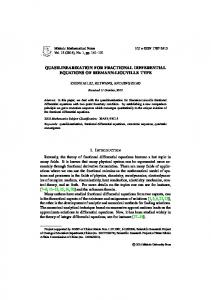
6.2 The Lorenz Equations In this section, we study the Lorenz equations [7, 14]. The equations are
x_ = �(y ? x)
(4)
y_ = �x ? y ? xz z_ = ? z + xy We study the system for � = 1, � = 2 and = 1. The system has three xed points (see [7, 14] for a detailed description of the dynamics of the system). The xed point at the origin is a saddle point with one dimensional unstable manifold. The other two xed points at (1,1,1) and (-1,-1,1) are stable. We compute the largest invariant set contained in the region R = [?3; 3] � [?3; 3] � [?3; 3]. It can be shown that k = 9 is a Lipschitz constant. The sample time is � = lnk2 (see discussion in Example 4.3). A graph is constructed on a grid of size 90 � 90 � 90. The algorithm of Section 2 is then used to compute the invariant set. In Figure 9, we show the cross sections of the invariant set for z = k, k 2 f?3; ?2; : : :; 2; 3g.
6.3 E�cient Storage Methods The main limitation of the grid method is the amount of memory required to store the grid points. The main limitation of the polyhedral method is that the iteration in the Reach Set Computation may never terminate. It may be possible to combine the desirable features of the two methods to obtain better e�ciency. Rather than storing the grid points explicitly, a set of grid points can be stored as a polyhedron using linear inequalities. Similary the termination problem in the Reach Set Computation for the polyhedral method may be addressed by using some features of the grid method. 21
−3
−2
−1
0
1
2
−3
3
3
−1
1
2
-3
3
-2
-1
0
1
2
3
3
z=2
3
z=1
2
2
2
2
2
2
1
1
1
1
1
1
0
0
0
0
0
0
−1
−1
−1
−1
-1
-1
−2
−2
−2
−2
-2
-2
−3 −3
y
−3 −2
−1
0
1
2
−3 −3
3
−3
−2
−1
0
1
2
−3
3
3
−1
−2
−1
0 x
1
0
1
2
-3 -3
3
-3 -2
-1
0
1
2
3
x
2
−3
3
3
3 z=0
y
−3 −2
x
y
0
3
z=3
y
−2
3
3
3
3
−2
−1
0
1
2
3 3
z = −1
z = −2
2
2
2
2
2
1
1
1
1
1
1
0
0
0
0
0
0
−1
−1
−1
−1
−1
−1
−2
−2
−2
−2
−2
−2
−3 −3
y
−3 −2
−1
0
1
2
−3 −3
3
−3 −2
−1
0 x
1
−1
0
1
x
−3
−2
2
2
3
y
−3 −3
2
−3 −2
−1
0 x
1
3
3
3 z = −3
y
2
2
1
1
0
0
−1
−1
−2
−2
−3 −3
−3 −2
−1
0 x
1
2
3
Figure 9: Computed Invariant Set for the Lorenz Equations
22
2
3
7 Conclucion We presented a method to compute Reachf (X0; t) | the reach set of the di�erential inclusion x_ 2 f (x) at time t. We also presented a method to compute the �-invariant sets of the inclusion x_ 2 f (x). We do this by relating the di�erential inclusion x_ 2 f (x) to an �-perturbation x_ 2 f�(x). This closely resembles concepts from perturbation theory, and structural stability in dynamical systems. In our future work, we will look into this relationship further. In particular, we would like to show that the presence of a property in x_ 2 f� (x) also implies the presence of that property for x_ 2 f (x) for some class of properties. Computing the invariant sets and reach sets is an important problem. It is nding increasing use in the study of hybrid systems (see [12, 13]). An important problem is to nd techniques to make the algorithms and methods presented in this paper more e�cient in terms of space and time usage.
References [1] R. Abraham, J.E. Marsden, and T. Raitu, Manifolds, Tensor Analysis, and Applications, Springer-Verlag, 1988. [2] R. Alur et. al., The Algorithmic Analysis of Hybrid Systems, Theoretical Computer Science, Feb. 1995. [3] R.Alur, C.Courcoubetis, T.A. Henzinger and P.-H. Ho, Hybrid automata: an algorithmic approach to the speci cation and veri cation of hybrid systems,Hybrid Systems, LNCS 736, Springer-Verlag. [4] J.P. Aubin and A. Cellina, Di�erential Inclusions, Springer-Verlag, 1984. [5] J.P. Aubin, Viability Theory, Birkhauser, 1991. [6] V. Borkar and P. Varaiya, �-Approximation of Di�erential Inclusion using Rectangular Di�erential Inclusion, Notes. [7] J. Guckenheimer and P. Holmes, Nonlinear Oscillations, Dynamical Systems, and Bifurcations of Vector Fields, Springer-Verlag, 1983. 23
[8] T. Henzinger, P. Kopke, A. Puri and P. Varaiya, What's Decidable About Hybrid Automata, STOCS 1995. [9] M. W. Hirsh and S. Smale Di�erential Equations, Dynamical Systems, and Linear Algebra, Academic Press, Inc., 1974. [10] X.Nicollin, A. Olivero, J. Sifakis, and S.Yovine, An Approach to the Description and Analysis of Hybrid Systems, Hybrid Systems, LNCS 736, Springer-Verlag, 1993. [11] A. Puri and P. Varaiya, Decidability of Hybrid System with Rectangular Differential Inclusions, CAV 94: Computer-Aided Veri cation, Lecture Notes in Computer Science 818, pages 95-104. Springer-Verlag, 1994. [12] A. Puri and P. Varaiya, Veri cation of Hybrid Systems using Abstractions, Hybrid Systems II, LNCS 999, Springer-Verlag, 1995. [13] A. Puri and P. Varaiya, Driving Safely in Smart Cars, California PATH Research Report UCB-ITS-PRR-95-24, July 1995. [14] C. Sparrow, The Lorenz Equations, Springer-Verlag, 1982. [15] P. P. Varaiya, On the Trajectories of a Di�erential System, in A.V. Balakrishnan and L.W. Neustadt, editor, Mathematical Theory of Control, Academic Press, 1967.
24