Approximation of smooth convex bodies by ... - The Institute

Approximation of smooth convex bodies by circumscribed polytopes with respect to the surface area K´aroly J. B¨or¨oczky∗, Bal´azs Csik´os† November 11, 2008

Abstract Let K be a convex body with C 2 boundary in the Euclidean dspace. Following the work of L. Fejes T´oth, R. Vitale, R. Schneider, P.M. Gruber, S. Glasauer and M. Ludwig, best approximation of K by polytopes of restricted number of vertices or facets is well-understood if the approximation is with respect to the volume or the mean width. In this paper we consider the circumscribed polytope P(n) of n facets with minimal surface area, and present an asymptotic formula in n for the difference of surface areas of P(n) and K.

Key words: polytopal approximation, extremal problems MSC 2000: 52A27, 52A40

1

Introduction

For any notions related to convexity in this paper, consult P.M. Gruber [21], R. Schneider [27] or T. Bonnesen and W. Fenchel [2]. For any quadratic form q, we write tr q to denote the sum, and det q to denote the product of the eigenvalues of q, respectively. As usual we call a compact convex set in Ek with non-empty relative interior a convex body in Ek . For a convex body K in Ed , we write V (K) to denote its volume, and S(K) to denote its surface area. When integrating on the boundary ∂K, we always do it with respect ∗

Supported by OTKA grants 049301 and 068398, and by the EU Marie Curie TOK project DiscConvGeo † Supported by OTKA grants 047102 and 67867

1

to the (d − 1)-dimensional Hausdorff measure (see K.J. Falconer [10] or C.A. Rogers [25] for definition and main properties). An X ⊂ ∂K is called Jordan measurable if its relative boundary on ∂K is of (d − 1)-measure zero. If K has C 2 boundary and x ∈ ∂K, then let Qx denote the second fundamental form at x, let H(x) = tr Qx , and let κ(x) = det Qx be the Gauß-Kronecker curvature. These notions naturally depend on K but we drop the reference to K. We say that K has C+k boundary if ∂K is C k and the Gauß-Kronecker is positive at each point. Best approximation of a convex body K with C 2 boundary by circumscribed polytopes with respect to the volume or the mean width has very extensive literature since the 1970’s (see the papers P.M. Gruber [16], [17], [18] and [20] for general surveys on related problems), and many of the major questions have been resolved. Here we only summarize the main results concerning the volume. P.M. Gruber [15] proved when ∂K is C+2 , and K. vol B¨or¨oczky, Jr. [3] in the general case that if P(n) is a polytope containing K with n facets that has minimal volume, then as n tends to infinity, we have V

vol (P(n) )

divd−1 − V (K) ∼ 2

µZ

∂K

κ(x)

1 d+1

dx

d+1 ¶ d−1

·

1 2

n d−1

(1)

where divd−1 > 0 depends only on d. P.M. Gruber [14] determined that √ 5 3 1 div1 = 12 and div2 = 18 , and it follows from the work of P.L. Zador [28] that 1 divd−1 = 2eπ d + O(ln d) (2) where the implied constant in O(·) is an absolute constant. In many cases important information available about the extremal bodies in polytopal approximation. If Ξn ⊂ ∂K has cardinality n for n ≥ d + 1, and f is a non-negative measurable function on ∂K whose integral on ∂K is positive, then {Ξn } is uniformly distributed with respect to f (compare S. Glasauer and R. Schneider [12]) provided that for any Jordan measurable X ⊂ ∂K, we have R f (x) dx #(X ∩ Ξn ) . lim = RX n→∞ n f (x) dx ∂K

In addition {Ξn } satisfies the Delone property (compare P.M. Gruber [19]) if there exists α, β > 0 depending on K and the sequence {Ξn } such that the −1 distance between any two points of Ξn is at least αn d−1 , and for any x ∈ ∂K −1 there exists y ∈ Ξn of distance at most βn d−1 from x. vol vol Now let Ξvol n be the family of points where the facets of P(n) touch P(n) . S. Glasauer and P.M. Gruber [13] proved that if ∂K is C+2 , then the {Ξvol n } 2

1

is uniformly distributed on ∂K with respect to κ(x) d+1 , and the result was extended to any convex body K with C 2 boundary by K. B¨or¨oczky, Jr. [3]. In addition, if ∂K is C+2 then P.M. Gruber [19] proved the Delone property for {Ξvol n }. The analogous results are also known in the case of approximation by circumscribed polytopes with respect to the mean width (see P.M. Gruber [21]). However if closeness is measured in terms of the surface area then the asymptotic formula was only known if K is ball (in that case approximation with respect to the volume and with respect to the surface area are equivalent). The goal of this paper is to fill this gap. It is especially desirable because if best approximation of smooth convex bodies is replaced by random approximation then we have essentially the same amount of information for all these three quermassintegrals (see K. B¨or¨oczky, Jr. and M. Reitzner [6]). We will assign certain number, which is denoted by div(q ∗ ), to any positive definite quadratic form q in d − 1 variables in Section 6. We prove (see (85)) divd−1 ≤ div(q ∗ ) ≤

d d−1

· divd−1

(3)

for any positive definite q where equality holds in the upper bound if the eigen values of q coincide. It follows by (2) that independently of the eigen values of q, we have 1 div(q ∗ ) = 2eπ d + O(ln d) (4) where the implied constant in O(·) is an absolute constant. If q is a positive semi-definite quadratic form in d − 1 variables that is not positive definite then we define div(q ∗ ) = divd−1 . In particular while div(q ∗ ) does depend on the eigen values of q, this dependence is rather ”light”. If d = 2, then the upper bound in (3) yields div(q ∗ ) = 2div1 = 1/6.

(5)

Unfortunately if d ≥ 3, then one cannot expect a ”nice” closed formula for div(q ∗ ) in terms of the eigen values of q. If d = 3 and τ2 ≥ τ1 > 0 are the eigen values of q then K.J. B¨or¨oczky and B. Csik´os [4] prove div(q ∗ ) =

2τ1 + τ2 4τ1 + 8τ2 + (4τ12 − 2τ1 τ2 + 7τ22 )1/2 · . 18(τ1 + τ2 ) [2τ1 + 4τ2 + (4τ12 − 2τ1 τ2 + 7τ22 )1/2 ]1/2

(6)

This formula could be expressed in terms of the trace and the determinant of q, but the new formula would be even more complicated.

3

Theorem 1.1 Given a convex body K in Ed , d ≥ 2, with C 2 boundary, if P(n) is a circumscribed polytope with n facets that has minimal surface area then as n tends to infinity, 1 S(P(n) ) − S(K) ∼ 2

µZ

∂K

d−1 d−1 1 div(Q∗x ) d+1 H(x) d+1 κ(x) d+1

dx

d+1 ¶ d−1

·

1 2

n d−1

.

We note that some cases of Theorem 1.1 have been already known. If K is a ball of radius r then S(P(n) ) = dV (P(n) )/r and S(K) = dV (K)/r, and hence P.M. Gruber’s (1) in [15] verifies Theorem 1.1. In addition if K is planar and its boundary is C+2 , then Theorem 1.1 is due to D.E. McClure and R.A. Vitale [9]. If K ⊂ P for the convex bodies K and P in Ed then their Hausdorff distance δH (P, K) is the maximal distance of the points of P from K (see Section 5). It is known (see K. B¨or¨oczky, Jr. [3]) that if K has C 2 boundary and P has at most n facets then δH (P, K) ≥ α2 where α is a positive n d−1

constant depending on K.

Theorem 1.2 For any convex body K in Ed , d ≥ 2, with C 2 boundary, if P(n) is a circumscribed polytope with n facets that has minimal surface area, and Ξn is a family of n points where the n facets of P(n) touch ∂K then d−1

d−1

1

(i) {Ξn } is uniformly distributed with respect to div(Q∗x ) d+1 H(x) d+1 κ(x) d+1 ; −2

(ii) δH (P(n) , K) ≤ βn d−1 where β depends on K; (iii) if moreover ∂K is C+2 then {Ξn } satisfies the Delone property. The rough idea of the proof of Theorem 1.1 is the same like for the volume difference as it was initiated by P.M. Gruber [15], and developed also by M. Ludwig [23]; namely, one thinks patches on ∂K being patches on suitable paraboloids, and uses the fact the power diagrams in Ed−1 correspond naturally to polytopal (piecewise linear) surfaces approximating paraboloids (see F. Aurenhammer [1]). In the cases of volume approximation, the problem is reduced (in a non-trivial way) to some properties of the second moment in Ed−1 as follows. Let C be a convex body in Ed−1 . For finite Ξ ⊂ C, if y ∈ Ξ, then we define the Dirichlet-Voronoi cell Πy of y to be the family of x ∈ C with kx − yk ≤ kx − zk for all z ∈ Ξ, and assign the second moment integral XZ kx − yk2 dx y∈Ξ

Πy

4

to Ξ, where k · k denotes the Euclidean norm. Now for large n, the question is the asymptotics of the minimum of the integral above as Ξ runs through all subset of C of cardinality at most n. This problem was solved by L. Fejes T´oth [11] if C is planar, and by P.M. Gruber [15] for higher dimensions. In the case of polytopal approximation with respect to the surface area, a similar problem arises in Ed−1 . Only in this case a positive definite quadratic form q in d − 1 variables is given, and we integrate not kx − yk2 , but q(x − y) above Πy in the expression above. The fact that we define the DirichletVoronoi cells with respect to the standard quadratic form, and integrate another quadratic form, causes much technical difficulty, especially when transforming the asymptotic result in Ed−1 to polytopal approximation in Ed . Concerning the structure of the paper, we discuss the above version of the moment problem in Section 2. For the later study, we need to understand related properties of convex hypersurfaces, which is done in Sections 3 and 4. Using these properties, we establish Theorem 1.2 (ii) and (iii) in Section 5, and prove the core result about approximation of paraboloids in Section 6. Next we discuss polytopal approximation of convex hypersurfaces of positive curvature in Section 7. Finally Theorem 1.1 is proved in Section 8, and Theorem 1.2 (i) in Section 9 using the method of K. B¨or¨oczky, Jr. [3]. Let us summarize notation. We write o to denote the origin in Ed , h·, ·i to denote the scalar product. Moreover let B d denote the unit ball centred at o. For non-colinear points u, v, w, the angle of the halflines vu and vw is ∠(u, v, w). Given a set X ⊂ Ed , the affine hull, the convex hull and the interior of X are denoted by affX, convX, and intX, respectively. The (d − 1)-dimensional Hausdorff measure of a measurable subset X of d E is denoted by |X|. if X is a subset of the boundary of a closed convex set in Ed with non-empty interior then we write relintX to denote its relative interior. In addition X is called Jordan measurable if it is bounded, and its relative boundary relbdX is of (d − 1)-measure zero. If in addition if X is the closure of relintX then X is called a convex hypersurface. Given two real functions f and g, we write f = O(g) if |f | ≤ c · g for some constant c depending only on the dimension d, and f = OΞ (g) if in addition c also depends on some object Ξ. Moreover ⌊t⌋ and ⌈t⌉ stand for the largest integer not larger, and the smallest integer not smaller, respectively, than t ∈ R.

5

2

A version of the Moment Lemma

While this section can be read independently from the rest of the paper, we work in Ed−1 because this is the setup how our main result Theorem 2.1 is applied in this paper. We write Υn to denote the family of all non-empty subsets of Ed−1 of cardinality at most n. P.M. Gruber [15] proved the existence of divd−1 > 0 depending only on d with the following property. If C is a Jordan measurable subset of Ed−1 , then as n tends infinity, we have Z d+1 1 min kx − yk2 dx ∼ divd−1 · |C| d−1 · 2 . min (7) Ξ∈Υn C y∈Ξ n d−1 If C is planar then (7) follows from the celebrated Moment Lemma of L. Fejes T´oth [11]. Far reaching generalizations of (7) where kx − yk2 is replaced by f (kx − yk) for some increasing function f with a “growth condition” are proved in P.M. Gruber [20]. For Ξ ∈ Υn and y ∈ Ξ, the Dirichlet-Voronoi cell of y with respect to Ξ and C is Π(y, Ξ, C) = {x ∈ C : kx − yk ≤ |x − z| for all z ∈ Ξ}. In particular in (7), we have Z XZ 2 min kx − yk dx = C y∈Ξ

y∈Ξ

Π(y,Ξ,C)

kx − yk2 dx.

Now let q be a positive definite quadratic form in d − 1 variables. For any finite subset Ξ of Ed−1 , we define XZ Ω(C, Ξ, q) = q(x − y) dx. y∈Ξ

Π(y,Ξ,C)

It follows by compactness argument that there exists an extremal Ξq,C,n ∈ Υn such that Π(y, Ξq,C,n , C) 6= ∅ for all y ∈ Ξq,C,n , and XZ q(x − y) dx. Ω(C, Ξq,C,n , q) = min Ω(C, Ξ, q) = min Ξ∈Υn

Ξ∈Υn

y∈Ξ

Π(y,Ξ,C)

We note that it is not clear whether Ξq,C,n has n elements. The reason is that if the eigenvalues of q are different then there exist C, Ξ and y such that Ω(C, Ξ ∪ {y}, q) > Ω(C, Ξ, q). Our main goal is to prove the following generalization of (7). 6

Theorem 2.1 For any positive definite quadratic form q in d − 1 variables there exists div(q) > 0 with the following property. If C is a Jordan measurable subset of Ed−1 , then as n tends infinity, we have d+1

−2

Ω(C, Ξq,M,n , q) ∼ div(q) · |C| d−1 · n d−1 . Before proving Theorem 2.1, we verify two auxiliary statements used in the proof. The first estimate is Ra consequence of the fact that given |M | for a Jordan measurable M ⊂ Ed−1 , M kyk2 dy is minimal if M is the (d − 1)-ball centred at o. Proposition 2.2 If M ⊂ Ed−1 is Jordan measurable then Z d+1 d−1 kyk2 dy ≥ · |M | d−1 . 2 M (d + 1) · |B d−1 | d−1 The second estimate is the H¨older inequality for positive a1 , . . . , ak and n1 , . . . , nk in the form d+1

−2

d+1

−2

d+1

−2

a1d−1 n1d−1 + . . . + akd−1 nkd−1 ≥ (a1 + . . . + ak ) d−1 (n1 + . . . + nk ) d−1 ,

(8)

where equality holds if and only if ai /aj = ni /nj for i, j = 1, . . . , k. Next we discuss two properties of Ω(M, Ξq,M,n , q) that will be also used in Section 6. The first is its homogeneity; namely, If λ > 0 and n ≥ 1, then Ω(λM, Ξq,λM,n , q) = λd+1 Ω(M, Ξq,M,n , q)

(9)

holds for any Jordan measurable M in Ed−1 . Now if M is a convex body in Ed−1 with o ∈ M , then for any ε ∈ (0, 1), (9) yields Ω((1 − ε)M, Ξq,M,n , q) ≥ (1 − ε)d+1 Ω(M, Ξq,M,n , q). In turn we deduce Ω(M \(1 − ε)M, Ξq,M,n , q) ≤ ε · 2d · Ω(M, Ξq,M,n , q).

(10)

Proof of Theorem 2.1: There exists some ω ≥ 1 such that kzk2 /ω ≤ q(z) ≤ ωkzk2 for any z ∈ Ed−1 . Since q is fixed, we set Ξq,M,n = ΞM,n . Let M be a Jordan measurable set that is the closure of its relative interior. It follows by Proposition 2.2 and the H¨older inequality (8), that if Ξ ∈ Υn , then X d+1 −2 d+1 (11) Ω(M, Ξ, q) ≥ γ1 |Π(y, Ξ, M )| d−1 ≥ γ1 |M | d−1 n d−1 , y∈Ξ

7

where γ1 depends on ω and d. There exists n ˜ depending on M such that if n>n ˜ , then in any face to face tiling of Ed−1 by cubes of (d − 1)-measure e to 2|M |/n, the number of the tiles intersecting M is at most n. Taking Ξ be the centres of these tiles shows that that there exists a γ˜ depending on ω and d such that if n > n ˜ , then −2

d+1

e q) ≤ γ˜ n d−1 |M | d−1 . Ω(M, ΞM,n , q) ≤ Ω(M, Ξ,

(12)

max diam[{y} ∪ Π(y, ΞM,n , M )] = 0.

(13)

Next we show that

lim

n→∞ y∈Ξq,M,n

Since M is the closure of its interior, for any δ > 0 there exists some η > 0 depending on δ and M such that if x ∈ M then |(x + δB d−1 ) ∩ M | > η. Let us assume that diam[{y0 } ∪ Π(y0 , ΞM,n , M )] ≥ 4δ for some y0 ∈ Ξq,M,n . In particular there exists some x0 ∈ M such that kx0 − yk ≥ 2δ for all y ∈ ΞM,n . If z ∈ (x + δB d−1 ) ∩ Π(y, ΞM,n , M ) for some y ∈ ΞM,n then q(z − y) ≥ δ 2 /ω, therefore Ω(M, ΞM,n , q) ≥ δ 2 η/ω. (14) In particular (12) yields (13). For W = [− 12 , 21 ]d−1 , we define 2

cn = n d−1 Ω(W, ΞW,n , q). It follows by (11) and (12) that div(q) = lim inf cn n→∞

is a positive and finite real number. Turning to C, we assume that C is the closure of its relative interior. It is suffient to prove that for any small ε > 0, there exist an N depending on ε, C, d and ω such that if n > N then d+1

−2

Ω(C, ΞC,n , q) = (1 + Oω (ε)) · div(q) · |C| d−1 · n d−1 .

(15)

It follows by the definition div(q), and applying (13) to M = W , that there exists some Nε depending on ε and d such that if n ≥ Nε , then (i) (1 − ε)div(q) ≤ cn ≤ (1 + ε)div(q); (ii) diam[{y} ∪ Π(y, ΞW,n , W ) < ε/2 for y ∈ ΞW,n . 8

We start with the lower bound implied in (15). Choose pairwise disjoint homothetic copies W1 , . . . , Wk of W in relintC whose total (d − 1)-measure is at least (1 − ε)|C|. It follows by (13) that there exists some Nε′ depending on ε, C and W1 , . . . , Wk such that for n > Nε′ and i = 1, . . . , k, any DirichletVoronoi cell Π(y, ΞC,n , C), y ∈ ΞC,n , intersects at most one Wi , and the the number ni of Dirichlet-Voronoi cells intersecting Wi is at least Nε for each i. In particular n1 + . . . + nk ≤ n. Therefore the condition (i) and the H¨older inequality (8) yield in this case that Ω(C, ΞC,n , q) ≥

k X i=1

Ω(W, ΞC,n , q) ≥ 2

≥ (1 − ε) div(q) · |C|

k X i=1

d+1 d−1

−2

d+1

(1 − ε)div(q) · |Wi | d−1 · nid−1 −2

· n d−1 .

(16)

Next we choose λ > 0, and homothets wi + λW , i = 1, . . . , m, with pairwise disjoint relative interiors such that the m homothetic copies of W cover C, and their total (d−1)-measure is at most (1+ε)|C|. We may assume that λ is small enough to ensure mNε > 1/ε. If n > mNε then let Ξn = ∪m i=1 (wi + λΞW,⌊n/m⌋ ). It follows by (ii) that if x ∈ wi + (1 − ε)λW , i = 1, . . . , m, then any closest point of Ξn to x lies in wi + λΞW,n . In particular m X i=1

−2

Ω(wi + (1 − ε)λW, Ξn , q) ≤ mcn λd+1 ⌊n/m⌋ d−1 d+1

−2

≤ (1 + ε)3 div(q)|C| d−1 n d−1 .

(17)

Let Wε = W \(1 − ε)W , and hence (10) yields −2

−2

Ω(Wε , ΞW,⌊n/m⌋ , q) ≤ ε · 2dc⌊n/m⌋ ⌊n/m⌋ d−1 ≤ ε · 3d div(q)(n/m) d−1 . For any x ∈ wi + λWε , i = 1, . . . , m, we consider a closest point y of Ξn to x, and closest point z of wi + λΞW,n . It follows by the definition of ω that q(x − y) ≤ ωkx − yk2 ≤ ωkx − zk2 ≤ ω 2 q(x − z). Therefore m X i=1

−2

Ω(wi + λWε , Ξn , q) ≤ ε · mω 2 3d div(q)λd+1 (n/m) d−1 d+1

−2

≤ ε · ω 2 4d div(q)|C| d−1 n d−1 . 9

(18)

Finally combining (16), (17) and (18) yields (15), and in turn completes the proof of Theorem 2.1. Q.E.D. Next we discuss a weak stability version of Theorem 2.1 if C is convex. Corollary 2.3 Let C ⊂ Ed−1 be convex body satisfying αrB d−1 ⊂ C ⊂ (r/α)B d−1 for α, r > 0, and let q be a quadratic form in d − 1 variables satifying ω −1 kzk ≤ q(z) ≤ ωkzk for ω ≥ 1. Then for any ε ∈ (0, 1), there exists n0 depending only on the parameters d, ε, α and ω such that if n > n0 , then d+1

−2

Ω(C, Ξq,C,n , q) = (1 + O(ε))div(q) · |C| d−1 · n d−1 , Π(y, Ξq,C,n , C) ⊂ y + εC.

(19) (20)

Proof: Let C1 , C2 be convex bodies in Ed−1 , and let q1 , q2 be positive definite quadratic forms in d − 1 variables satisfying (1 + ε)−1 C1 ⊂ C2 ⊂ (1 + ε)C1 and (1 + ε)−1 q1 ≤ q2 ≤ (1 + ε)q1 for ε ∈ (0, 1). Writing Ξi = Ξqi ,Ci ,n , we deduce by (9) that Ω(C2 , Ξ2 , q2 ) ≥ Ω((1 + ε)−1 C1 , Ξ2 , (1 + ε)−1 q1 ) ≥ (1 + ε)−(d+2) Ω(C1 , Ξ1 , q1 ). In particular for given n, Ω(C, Ξq,C,n , q) is a continuous function of q and a convex body C in Ed−1 . To prove both statements in Corollary 2.3, we may assume that αB d−1 ⊂ C ⊂ (1/α)B d−1

(21)

by homogeneity. Under this assumption, the space of all possible C and q is compact, therefore (19) follows from Theorem 2.1. Since the η in (14) in the proof of Theorem 2.1 depends only on δ, d and α by (21), we deduce (20) from (14) and (19). Q.E.D. Remark 2.4 It follows from Theorem 2.1 that if q1 and q2 are quadratic forms in d − 1 variables satifying (1 + ε)−1 q1 ≤ q2 ≤ (1 + ε)q1 for ε ∈ (0, 1), then (1 + ε)−1 div(q1 ) ≤ div(q2 ) ≤ (1 + ε)div(q1 ). In general, we only have the following estimate for div(q) in terms of divd−1 .

10

Lemma 2.5 If q is a positive definite quadratic form in d−1 variables whose minimal eigenvalue is τ , then tr q τ · divd−1 ≤ div(q) ≤ · divd−1 , d−1 where equality holds in the upper bound if the eigen values of q coincide. Proof: The lower bound readily holds. To prove the upper bound on div(q), Pd−1 we may assume that q(y) = j=1 τj t2j for y = (t1 , . . . , td−1 ). We write pj y to denote the j th coordinate of y ∈ Ed−1 . Let W = [− 21 , 21 ]d−1 . According to (7), if ε > 0 and n is large then there exists Ξ = {y1 , . . . , yn } ∈ Υn such that Z n −2 min kx − yi k2 dx ≤ (1 + ε) · divd−1 · n d−1 . W i=1

Writing Πi = Π(yi , Ξ, W ), we define n Z X αj = [pj (x − yi )]2 dx for j = 1, . . . , d − 1. i=1

Πi

Now there exists a permutation σ : {1, . . . , d − 1} → {1, . . . , d − 1} satisfying d−1 X j=1

τj · ασ(j)

d−1 tr q X · αj . ≤ d − 1 j=1

Therefore writing Ψ to the linear transformation with pj Ψy = pσ(j) y, we have ΨW = W and n Z X −2 (1 + ε) tr q q(x − yi ) dx ≤ · divd−1 · n d−1 . d−1 i=1 Πi In turn we conclude Lemma 2.5.

Q.E.D. √ 5 3 18

1 and div2 = according to P.M. Gruber [14], We note that div1 = 12 and it follows from the work of P.L. Zador [28] that

divd−1 =

1 2eπ

d + O(ln d)

(22)

where the implied constant in O(·) is an absolute constant. It follows from Lemma 2.5 that if d = 2 and q(x) = κx2 then div(q) = κ/12. In addition the value of div(q) has been determined in K.J. B¨or¨oczky, B. Csik´os [4] if q has two variables and the eigen values are not too different: If q is a positive definite quadratic form in two variables with eigenvalues τ < κ ≤ 2.4τ , then √ τ [4κ + (4κ2 − 6τ κ + 3τ 2 )1/2 ] div(q) = . (23) 18[2κ + (4κ2 − 6τ κ + 3τ 2 )1/2 ]1/2 11

3

Convex hypersurfaces

In this section we start the study of convex hypersurfaces. Let us discuss first some notions associated to a positive definite quadratic q form in d − 1 variables. We can choose a orthonormal bases for Ed−1 such that if y = 2 (y1 , . . . , yd−1 ) ∈ Ed−1 then q(y) = τ1 y12 + . . . + τd−1 yd−1 where τ1 , . . . , τd−1 are the associated eigen values. Using this notation, we assign the positive definite quadratic form q ◦ to q defined by 2 2 q ◦ (y) = τ12 y12 + . . . + τd−1 yd−1 .

We say that a convex hypersurface X ⊂ Ed is proper if convX is a convex body in Ed . In this case we write uX (x) to denote some exterior unit normal at x ∈ relintX that is unique for all x ∈ relintX but of a set of (d − 1)measure zero. When integrating over X, we always do it with respect to the (d − 1)-dimensional Hausdorff measure. If the closest point x of convX to some y lies in X then we write πX (y) = x. We note that kπX (y) − πX (y ′ )k ≤ ky − y ′ k, hence if πX is defined and injective on some convex hypersurface Y then |πX (Y )| ≤ |Y |, and πX (Y ) is also a convex hypersurface. We will also meet the following setup: Given convex hypersurfaces X, Y such that X = πX (Y ), let Z ⊂ relintX be a convex hypersurface. Then the subset Z ′ of Y satisfying πX (Z ′ ) = Z is a convex hypersurface, as well. We note if L is the boundary of a closed convex set in Ed with non-empty interior then we also write πL to denote the closest point map into L. If the convex hypersurface Y ⊂ Ed is the union of F1 , . . . , Fk such that each Fi is a Jordan measurable subset of some hyperplane and has positive (d − 1)-measure, and affF1 , . . . , affFk are pairwise different then we call Y a convex polytopal hypersurface, and F1 , . . . , Fk the facets of Y . If affFi for i = 1, . . . , k touches some proper convex hypersurface X then we say that Y is circumscribed around X. For certain calculations it is useful to consider patches as graphs of functions. We think Ed as Ed−1 × R where x = (y, t) is the point of Ed corresponding to y ∈ Ed−1 and t ∈ R, and define B d−1 = B d ∩ Ed−1 . We write ξ = (o, −1) to denote the ”downwards” unit normal to Ed−1 . If C ⊂ Ed−1 has non-empty interior in Ed−1 , and θ : C → R is any function then the graph of θ is Γ(θ) = {(y, θ(y)) : y ∈ C} ⊂ Ed . 12

(24)

In particular the graph of any convex function defined on convex body in Ed−1 is a convex hypersurface. We say that a convex hypersurface X is a C 2 convex hypersurface if any point of X has an open neighbourhood on X that is congruent to the graph of some C 2 function. In order to define the principle curvatures at x0 ∈ relintX, we may assume that Ed−1 is the tangent hyperplane to X at x0 = (y0 , 0), and a neighbourhood X0 ⊂ X of x0 is the graph of a C 2 function θ on an open convex Ψ ⊂ Ed−1 . Then the principle curvatures κ1 (x0 ), . . . , κd−1 (x0 ) of X at x0 are the eigenvalues of the symmetric matrix corresponding to the quadratic form representing the second derivative of θ at y0 . For x ∈ X, we define σ0 (x) = 1, and write σj (x) to denote the j th symmetric polynomial of the principal curvatures for j = 1, . . . , d − 1; namely, X σj (x) = κi1 (x) · . . . · κij (x). 1≤i1 0 depending on K with the following property (see say K. Leichtweiß [22]): If x ∈ ∂K then there exists a ball that lies 13

in K, is of radius η, and touches ∂K from inside at x. Since any tangent hyperplane to relint Y avoids int K, if x ∈ relint X then huX (x), uY (xY )i ≥

η . η+̺

(27)

Therefore (25) yields (26).

4

Some basic properties of graphs of convex functions

The main goal of this section is to observe some basic properties of convex hypersurfaces that are needed in the paper. First we introduce the notions that we discuss until (45), and state the conditions (28) to (43) on these notions. Let q be a positive definite quadratic form in d − 1 variables, and let ω > 1 satisfy ω −1 ≤ ·kzk2 q(z) ≤ ω · kzk2

for z ∈ Ed−1 .

(28)

In addition, let 1 ε ∈ (0, 20ω 2 ).

(29)

We investigate a non-negative C 2 function θ defined on the (d−1)-dimensional convex body C, where √ C ⊂ ε B d−1 with o ∈ relintC. (30) We write ly to denote the linear form and qy to denote the quadratic form representing the second derivative of θ at y ∈ C. We assume that ¾ θ(o) = 0 and lo (z) = 0; for z ∈ Ed−1 . (31) q(z) − ε · kzk2 ≤ qy (z) ≤ q(z) + ε · kzk2 We define X ′ = Γ(θ). It follows by the Taylor formula for y, z ∈ C that θ(z) − θ(y) − ly (z − y) = 12 qy+t(z−y) (z − y) for t ∈ (0, 1); = 12 q(z − y) + O(ε) ky − zk2 ; klz − ly k2 = q ◦ (z − y) + O(εω) kz − yk2 .

(32) (33) (34)

If y ∈ relintC and x = (y, θ(y)) then uX ′ (x) = (1 + kly k2 ) 14

−1 2

· (ly , −1).

(35)

It follows by (30), (34) and (35) that if x, x′ ∈ relintX ′ for x = (y, θ(y)) and x′ = (y ′ , θ(y ′ )) then huX ′ (x), uX ′ (x′ )i = 1 − 21 q ◦ (y − y ′ ) + O(εω 2 ) ky − y ′ k2 .

(36)

If x′ = o then we have a more precise formula. Since X ′ does not intersect 1 the interior of the ball of radius 2ω centred at −1 ξ, there is a point z on the 2ω boundary of this ball where the exterior unit normal is uX ′ (x) and kπEd−1 zk ≤ √ 2 ε. We conclude hξ, uX ′ (x)i ≥ (1 + 8ω 2 ε)

−1 2

≥ 1 − 4ω 2 ε for x ∈ relintX ′ .

(37)

It also follows that if z ∈ C and πX ′ z is well defined then 3 ˜ ˜ > 1 depending on ω and d. kz − πE d−1 πX ′ zk ≤ ℵkzk for ℵ

(38)

Recalling that σj (x) denotes the j th symmetric polynomial of the principal curvatures x ∈ relintX ′ for j = 1, . . . , d − 1, we have H(x) = tr q + O(ε); κ(x) = det q + O(εω d−2 ); σj (x) = O(ω j ).

(39) (40) (41)

Next let Y be a convex hypersurface such that πX ′ is defined on Y and it is injective, and let X = πX ′ (Y ). We will assume that if x ∈ X then rX,Y (x) ≤ ̺ where ̺ ∈ (0, ε); √ kx − x′ k > 2 ̺ω for x ∈ X and x′ ∈ relbd X ′ .

(42) (43)

Since all eigen values of qy are at most 2ω for any y ∈ C, there is a ball of 1 radius 2ω touching X from inside at any x ∈ X such that the ball intersects X only in x, which in turn yields huX (x), uY (xY )i−1 ≤ 1 + 2̺ω.

(44)

As a rough estimate, (25) yields the analogue of (26); namely, |Y | − |X| = O(̺ω) · |X|.

(45)

We also consider a polytopal hypersurface Z circumscribed around X ′ such that Z is the graph of a convex function h defined on a subset of C. Assume that a facet F of Z touches X ′ in (y0 , θ(y0 )) for y0 ∈ C, and let x ∈ F of the form x = (y, h(y)), y ∈ C. Now d(x, X ′ ) is at most the distance 15

of x from x′ = (y, θ(y)), and at least the distance of x from the tangent plane to X ′ at x′ . In particular the Taylor formula (32) and (37) yield 1−5ω 2 ε 2

· q(y − y0 ) ≤ d(x, X ′ ) ≤

1+ωε 2

· q(y − y0 ).

(46)

It also follows that if some facet of Z touches X ′ at (z0 , θ(z0 )) for z0 ∈ C then 1 q(y − z0 ) ≤ q(y − y0 ) ≤ 2q(y − z0 ). (47) 2 In the final part of the section, our main goal is to establish Lemma 4.2 that allows us to shift between patches on smooth convex hypersurfaces. First we verify a simple technical statement. Proposition 4.1 Let z1 , z2 ∈ Ed−1 such that kz2 − z1 k ≤ τ for some τ > 0, d−1 and let Y be the such √ graph of a convex positive function on z1 + 2τ B √ that zi −yi 3 huY (y), ξi ≥ 2 for y ∈ Y . If y1 , y2 ∈ Y satisfy that h kzi −yi k , ξi ≥ 23 for i = 1, 2 then ky1 − y2 k ≤ 2 · [kz1 − z2 k + kz1 − y1 k · ∠(z1 − y1 , o, z2 − y2 )]. Proof: We define y1′ ∈ Y by the property that the vectors z1 − y1′ and z2 − y2 are parallel, and prove ky1 − y1′ k ≤ 2 kz1 − y1 k · sin ∠(y1 , z1 , y1′ ).

(48)

Let σ be the arc that is the intersection of the triangle y1 z1 y1′ and Y , and let y be the point of σ farthest from the segment y1 y1′ . Then the tangent line to √ 3 ′ σ at y is parallel to the line y1 y1 , hence huY (y), ξi ≥ 2 yields that the angle of y1′ − y1 and ξ is between π3 and 2π . Thus the angle of the triangle z1 y1 y1′ 3 , therefore the law of sine implies (48). at y1′ is between π6 and 5π 6 Now an argument as above shows that ky2 − y1′ k ≤ 2 kz2 − z1 k, which in turn yields Proposition 4.1. Q.E.D. Let us set up the notation used in Lemma 4.2. Let q be a positive definite quadratic form in d − 1 variables with ω −1 kzk ≤ q(z) ≤ ωkzk for z ∈ Ed−1 . 1 8 For ε√∈ (0, 16ω 2 ) and ̺ ∈ (0, ε ), let the convex functions h1 , h2 , f1 , f2 defined 20 ̺ on ε B d−1 satisfy the following properties: We have f2 (o) = 0, f2′ (o) = 0, √ 8 ̺ f1 and f2 are C 2 . In addition if y ∈ ε B d−1 then

h1 (y) ≤ f1 (y) ≤ f2 (y) ≤ h1 (y) + ̺ and f1 (y) ≥ 0, 16

(49)

and writing qi,y to denote the quadratic form representing the second derivative of fi at y for i = 1, 2, we have q(z) − ε8 · kzk2 ≤ qi,y (z) ≤ q(z) + ε8 · kzk2

for z ∈ Ed−1 .

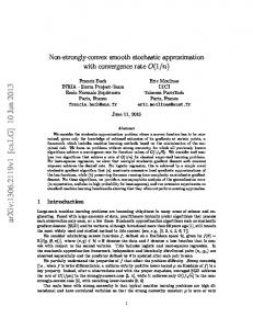
For i = 1, 2, we define Yi = Γ(hi ) and Xi = Γ(fi ) (see Figure 1). We assume that Yi is a polytopal hypersurface circumscribed around Xi , and the affine hulls of the of the facets of Y1 and Y2 are in bijective correspondence in a way that the affine hulls of the corresponding facets are parallel. In particular h1 (y) ≤ h2 (y) for y ∈

√ 20 ̺ ε

B d−1 . X2

Y2

X1

Y1 Ed−1

Figure 1:

1 Lemma 4.2 Given ω > 1 and d, there exists ε0 ∈ (0, 16ω 2 ) depending on d and ω with the following properties. Using the notation as above, if C ⊂ Ed−1 √ √ 4 ̺ ̺ ei = πX (C), is a compact convex satisfying 4ε B d−1 ⊂ C ⊂ ε B d−1 , and X i ei = πX (Yei ) for i = 1, 2, then moreover Yei denote the subset of Yi satisfying X i

ei | = [1 + O(ε)] · |C| for i = 1, 2; |X e1 | = |Ye2 | − |X e2 | + O(ε̺) · |C|. |Ye1 | − |X

(50) (51)

Proof: Readily if ε0 is sufficiently small then

ei ), πEd−1 (Yei ) ⊂ 2C, i = 1, 2. πEd−1 (X

√

It follows by (37) that if ε0 is sufficiently small then huXi (x), ξi ≥ 23 for any x ∈ relintXi . In addition if y = (z, hi (z)) for z ∈ 2C, i = 1, 2, and u is an exterior unit normal to Yi at y then d(y, Xi ) ≤ ̺ and (32) yield√that there √ exists x ∈ Xi ∩ (y + 4 ω̺ B d ) with u = uXi (x), hence hu, ξi ≥ 23 , as well. 17

In addition the conditions on h1 , h2 , f1 , f2 and applying (32) to f1 , f2 yield that h1 (z) ≥ h2 (z) > 0 if z ∈ (2C)\( 21 C); if z ∈ 2C; f2 (z) ≤ 64ω̺ ε2 6 f2 (z) − f1 (z) ≤ 64ε ̺ if z ∈ 2C; h2 (z) − h1 (z) ≤ 64ε6 ̺ if z ∈ 2C.

(52) (53) (54) (55)

Therefore combining (45), (53) and 64ω̺ · ω < ε leads to (50). ε2 ′ For z ∈ C, we define θYi (z) = Yi ∩ conv{z, πXi (z)} for i = 1, 2, θX (z) = 1 ′ X1 ∩ conv{z, πX2 (z)} and θY1 (z) = Y1 ∩ conv{z, πX2 (z)}, which points exist by (52). In particular Yei = θYi (C) for i = 1, 2, and the relative boundaries of e1 and θ′ (C) are the corresponding images of ∂C. We deduce Ye1 , θY′ 1 (C), X X1 by (45), (54) and (55) that if ε0 is small enough then

Now we prove

′ e2 | = O(ε̺) · |C|; |θX (C)| − |X 1 |θY′ 1 (C)| − |Ye2 | = O(ε̺) · |C|.

(56)

′ e1 | − |θX |X (C)| = O(ε̺) · |C|; 1 |Ye1 | − |θY′ 1 (C)| = O(ε̺) · |C|.

(58)

Let z ∈ ∂C. It follows by (53) that kz − θX1 (z)k ≤ √

64ω̺ , ε2

(57)

(59) and the discussion

z−θ (z) above shows that h kz−θYY1 (z)k , ξi ≥ 23 . In addition the analogous two inequal1 ′ ities hold for πX1 (z), θX and θY′ 1 in place of θX1 . Next let xi = πXi (z), 1 ′ i = 1, 2. Since d(θX (z), X2 ) ≤ 64ε6 ̺ by (54), and there exists a ball of 1 1 radius 4ω touching X2 from inside at x2 , we deduce that the angle α2 of √ ′ ′ (z) − x1 k = uX2 (x2 ) and uX1 (θX (z)) is O(ε3 ω ̺). It follows that kθX 1 1 3 √ ′ 2 2 3 O(ε ω ̺)kθX1 (z) − zk = O(εω ̺ ), hence the angle α1 of uX1 (x1 ) and 3 ′ uX1 (θX (z)) is O(εω 3 ̺ 2 ) according to (36). Therefore choosing ε0 small 1

enough, we have

′ ∠(z − πX1 (z), o, z − θX (z)) = ∠(z − θY1 (z), o, z − θY′ 1 (z)) 1 √ ε2 ̺ 3 3√ . (60) ≤ α1 + α2 = O(ε ω ̺) < 128ω

We provide the rest of argument only for (59), and (58) can be similarly proved. It follows by Proposition 4.1, (60) and kθY1 (z) − zk ≤ 64ω̺ that ε2 3

kθY′ 1 (z) − θY1 (z)k ≤ ̺ 2 , 18

(61)

hence (59) is a consequence of ¯ ´¯ ³ 3 ¯ d ¯ 2 ¯Y1 ∩ θY1 (relbdC) + ̺ B ¯ = O(ε̺) · |C|. √

(62)

̺

To prove (62), let τ = 4ε , and let z1 , . . . , zk ∈ ∂C be a maximal family of 3 3 points with the property that kzi − zj k ≥ 3̺ 2 for i 6= j. Since zi + ̺ 2 B d−1 are pairwise disjoint for i = 1, . . . , k, and each is contained in the difference 3

of (1 +

̺2 τ

3 2

) C and (1 − ̺τ ) C, we deduce that µ 3¶ 3 3 2 k = O ̺τ · |C| · (̺ 2 )−(d−1) = O(ε̺) · |C| · (̺ 2 )−(d−1) .

(63)

3

Now let y ∈ Y1 satisfy that ky − θY1 (z)k ≤ ̺ 2 for some z ∈ ∂C. There 3 3 exists some zi such that kzi − zk ≤ 3̺ 2 , hence kπX1 (zi ) − πX1 (z)k ≤ 3̺ 2 . In particular (36) implies that the angle of zi − θY1 (zi ) and z − θY1 (z), which is 3 the angle of uX1 (πX1 (zi )) and uX1 (πX1 (z)) is at most 4ω̺ 2 (after choosing 1 ε0 small enough). Thus kz − θY1 (z)k ≤ 8ω and Proposition 4.1 yield that 3 3 kθY1 (zi ) − θY1 (z)k ≤ 7ω̺ 2 , hence kθY1 (zi ) − yk ≤ 8̺ 2 . We deduce by (63) that k ¯ ¯ ³ ´¯ ´¯ ³ X 3 3 ¯ ¯ ¯ d ¯ 2 ¯Y1 ∩ θY1 (∂C) + ̺ B ¯ ≤ ¯Y1 ∩ θY1 (zi ) + 8̺ 2 B d ¯ i=1

3

≤ k · S(8̺ 2 B d ) = O(ε̺) · |C|.

We conclude (62), and in turn (59) and (58). Finally combining (56), (57), (58) and (59) yields (51), and in turn Lemma 4.2. Q.E.D.

5

The Delone property of the extremal body

In this section we establish Theorem 1.2 (ii) and (iii). For x ∈ En and a compact X ⊂ En , we write d(x, X) to denote the minimal distance between x and the points of X. If X and Y are compact sets in En then their Hausdorff distance is ½ ¾ δH (X, Y ) = max max d(x, Y ), max d(y, X) . x∈X

y∈Y

To verify our main result Lemma 5.2, we need Proposition 5.1. We write Hd−2 (·) to denote the (d − 2)-dimensional Hausdorff measure. 19

Proposition 5.1 If M ⊂ N are convex bodies in Ed such that for some x ∈ ∂M , there exists a ball B ⊂ M of radius η touching ∂M at x, and x + δ · u∂M (x) ∈ N for 0 < δ < η then S(N ) − S(M ) > c · η

d−3 2

·δ

d+1 2

where c > 0 depends only on d. Proof: We may assume that x = o, Ed−1 is the supporting hyperplane to M at x, and u∂M (x) = ξ. We define C = Ed−1 ∩ N , x0 = x + δ · u∂M (x), and Y to be the convex hypersurface that is the union of the segments of the form conv{x0 , y} for y ∈ ∂C. In addition we define uy ∈ Ed−1 to be an exterior unit normal to ∂C at y ∈ ∂C, and the radial function ̺(z) > 0 by the property ̺(z) · z ∈ ∂C for z ∈ B d−1 . The existence of B yields that √ ̺(z) > 12 ηδ for all z ∈ B d−1 . Therefore Z q 1 huy , yi2 + δ 2 − huy , yi dy S(N ) − S(M ) ≥ |Y | − |C| = d − 1 ∂C Z Z ̺(z)d−3 δ2 1 δ2 dy = dz > 4(d − 1) ∂C huy , yi 4(d − 1) ∂B d−1 hu̺(z)·z , zi2 Hd−2 (∂B d−1 ) d−3 d+1 ·η 2 ·δ 2 ≥ 4(d − 1) where the integration always occurred with respect to Hd−2 (·).

Q.E.D.

We prove Theorem 1.2 (ii) and (iii) as part of Lemma 5.2. Lemma 5.2 Let K be a convex body in Ed with C 2 boundary, let P(n) be a circumscribed polytope with n ≥ d + 1 facets that has minimal surface area, and let X ⊂ ∂K be a convex hypersurface such that the Gauß-Kronecker curvature is positive at the points of X. Then δH (P(n) , K) ≤ β02 , and n d−1

if F is a facet of P(n) with π∂K (F ) ∩ X 6= ∅ and F touches K in x then diamF ≤ β1 , and F contains a (d − 1)-ball with centre x and radius α1 n d−1

n d−1

where α, β, β0 are positive, β0 depends on K, and α, β depend on X and K.

Proof: Readily it is sufficient to consider the case when n is large. It is known (see say K. Leichtweiß [22]) that for suitable η > 0 depending on K, if x ∈ ∂K then there exists a ball that lies in K, is of radius η, and touches ∂K from inside at x. In addition we write Lx to denote the supporting hyperplane to K at x ∈ ∂K, and L+ x to denote the half space containing K. During the 20

proof of Lemma 5.2, α1 , α2 , . . . and β1 , β2 , . . . denote positive constants that depend on X and K. Our first task is to establish the order S(P(n) ) − S(K) (see (64) and (69). According to K. B¨or¨oczky, Jr. [3] (or E.M. Bronˇste˘ın and L.D. Ivanov [8] in a more general framework), there exists a polytope Q(n) circumscribed around K with n facets satisfying δH (K, Q(n) ) < β12 , therefore n d−1

S(P(n) ) − S(K) ≤ S(Q(n) ) − S(K)
1 depending on X and K with the following two properties: First if y ∈ X2 then H(y) = σ1 (y) > ω −1 . Secondly assuming that Φx = (x + γ B d ) ∩ ∂K intersects X1 for x ∈ ∂K, we have Φx ⊂ X2 , and if y ∈ Φx then tan ∠(u∂K (x), o, u∂K (y)) ≤ ω · ky − xk; ω · ky − xk2 ≤ r∂K,Lx (y) ≤ ω · ky − xk2 . −1

(67) (68)

We write F1 , . . . , Fn to denote facets of P(n) , and xi to denote a point of ∂K where Fi touches K. We assume that π∂K (Fi ) ∩ X 6= ∅ if and only if i ≤ k, and Fj intersects some Fi with i ≤ k if and only if i ≤ k0 . According to (66) and (68), we may assume that n is large enough to ensure that if i ≤ k and Fj intersects Fi then π∂K (Fi ) ∪ π∂K (Fj ) ⊂ Φxi .

21

We write Ci to denote the orthogonal projection of π∂K (Fi ) into Lxi , and deduce by (25) and Proposition 2.2 that if i ≤ k then Z |Fi | − |π∂K (Fi )| > r∂K,Lxi (y)H(y) dy π∂K (Fi ) Z Z −2 2 ω −2 · kz − xk2 dz > ω · ky − xk dy > π∂K (Fi )

> α2 · |Ci |

Ci

d+1 d−1

> α3 · |π∂K (Fi )|

d+1 d−1

.

Therefore the H¨older inequality (8) yields S(P(n) ) − S(K) ≥

k X i=1

d+1

[|Fi | − |π∂K (Fi )|] ≥

α3 · |X| d−1 2

k d−1

.

(69)

Comparing with (64) leads to k > α4 n. We are ready to face directly the Delone property. It follows by (68) that √ (70) kz − xi k < ωδ if i ≤ k0 and z ∈ Fi , which in turn yields that −2

−2

δ ≥ α5 · k d−1 ≥ α5 · n d−1 .

(71)

For any i = 1, . . . , k0 , we write νi to denote the minimal distance of the (d − 2)-faces of Fi from xi , and define ν = mini=1,...,k νi . Readily −1

−1

ν ≤ β4 · k d−1 ≤ β5 · n d−1 ,

(72)

and let m ≤ k satisfy ν = νm . We observe that Pe = P(n) ∩ L+ x ˜ has n + 1 facets, and d+1 (73) S(P(n) ) − S(Pe) > α6 · δ 2 according to Proposition 5.1. We define Fem = Fm ∩ Pe, and ´ ³ + , P ′ = L+ ∩ ∩ i6=m Lx x ˜ i i≤n

which is a polytope circumscribed around K with n facets. We write Y to e e denote the part of ∂ Pe cut off by Lxm . If √ G is a facet of P intersecting Fm and touching K in y then ky − xm k < 2 ωδ (see (70)), hence (67) yields 3

1

tan ∠(u∂K (xm ), o, u∂K (y)) ≤ 2ω 2 · δ 2 . 22

(74)

We define w = xm +2ωδ·u∂K (xm ), thus Y is contained in C = conv{w, Fem }. In addition there exists some xj with j ≤ k0 , j 6= m, such that A = Lxm ∩ Lxj contains a (d − 2)-face of Fm , and the distance of xm from A is ν. Since kxj − xm k ≤ (1 + ω 2 )ν follows by (68), (67) implies tan ∠(u∂K (xm ), o, u∂K (xj )) ≤ 2ω 3 · ν. ′ ′ ′ e We define C ′ = C ∩ L+ xj and Y = ∂C \relintFm , hence Y ⊂ C yields

(75)

S(P ′ ) − S(Pe) = |Y | − |Fem | ≤ |Y ′ | − |Fem |.

(76)

hu∂K (xm ), uY ′ (y)i−1 ≤ 1 + 8ω 3 · δ.

(77)

It follows by (74) that if y ∈ relintY ′ and n is large then

In addition if y ∈ relint(Y ′ ∩ Lxj ) then (75) yields hu∂K (xm ), uY ′ (y)i−1 ≤ 1 + 8ω 6 · ν 2 . √ Next we prove that if δ > 2dω 3 ν then ´ ³ 3 1 − 2ω√δν · (Fem − xm ) + xm ⊂ πLxm (Y ′ ∩ Lxj ).

(78)

(79)

3 Let x ∈ (1 − 2ω√δνν ) · (Fem − xm ) + xm , and let y ∈ Y and z ∈ Y ′ ∩ Lxj satisfy that πLxm (y) = πLxm (z) = x. Now the definition of Y shows that √ 3 kz − xk ≥ 2ω√δν · 2ωδ = 4ω 4 · ν δ. (80)

√ 7 1 Since the distance of x from A is at most 2 ωδ, we deduce ky −xk ≤ 4ω 2 νδ 2 by (75), which inequality combined with√(80) yield (79). In turn we conclude d−1 by (77), (78) and |Fem | ≤ β6 δ 2 that if δ > 2dω 3 ν then ·³ µ ´d−1 ¶ ¸ ´d−1 ³ d−1 3ν 3ν 2 ′ 2ω 2ω · δ . (81) · ν + 1 − 1 − √δ |Y | − |Fem | ≤ β7 δ 2 · 1 − √δ Since S(P(n) ) ≤ S(P ′ ), combining (73), (76) and (81) leads to h i d+1 d−1 3 √ ν ·δ . α6 · δ 2 < β7 δ 2 · ν 2 + 2dω δ

Therefore δ < β8 ν 2 in any case, hence the estimates (71) and (72) complete the proof of Lemma 5.2. Q.E.D. 23

6

Approximating paraboloids

If K is a convex body with C 2 boundary, and the Gauß-Kronecker curvature is non-zero at x ∈ ∂K, then a small neighbourhood of x on ∂K can be very well approximated by a patch on a parabaloid. Using Lemma 4.2, polytopal approximation of this neighbourhood of x can be related to polytopal approximation of the patch on the paraboloid. Therefore in this section we consider the latter problem. Let q be a positive definite quadratic form in d − 1 variables, and let ω ≥ 1 satisfy ω −1 · kzk2 ≤ q(z) ≤ ω · kzk2

for z ∈ Ed−1 .

(82)

We choose a orthonormal bases for Ed−1 such that if y = (t1 , . . . , td−1 ) ∈ Ed−1 then q(y) = τ1 t21 + . . . + τd−1 t2d−1 , and hence ω −1 ≤ τi ≤ ω for each τi . We assign the positive definite quadratic form q ∗ to q defined by ¶ d−1 µ X 1 τi q (y) = kyk + · t2i . · q(y) = 1+ tr q τ + . . . + τ 1 d−1 i=1 ∗

2

(83)

The role of q ∗ will be explained by Lemma 6.1. We frequently estimate q ∗ (z) by kzk2 ≤ q ∗ (z) ≤ 2 · kzk2 . (84) Since tr q ∗ = d, Lemma 2.5 yields

divd−1 ≤ div(q ∗ ) ≤

d d−1

· divd−1 ,

(85)

where equality holds in the upper bound if the eigen values of q coincide. In Lemma 6.1, we further consider the graph X ′ the graph of 21 q above Ed−1 , and a compact convex set C in Ed−1 with rB d−1 ⊂ C ⊂ 16rB d−1

(86)

for some r > 0. In addition let X = πX ′ (C). Lemma 6.1 For ω ≥ 1 and d ≥ 2, there exist ε0 , ℵ > 0 with the √ following properties. If ε ∈ (0, ε0 ), and q, C, X ′ and X as above, and C ⊂ ε B d−1 , and n > n0 where n0 depends on ω, d and ε, then we have (i) and (ii) below. (i) If Y is a polytopal convex hypersurface circumscribed around X ′ satisfying X = πX ′ (Y ), and Y has at most n facets then ∗

1

d+1

−2

) · (tr q) · (det q) d−1 |C| d−1 · n d−1 . |Y | − |X| ≥ (1 − ℵε) div(q 2

24

(ii) There exists a polytopal convex hypersurface Y circumscribed around X ′ with at most n facets such that X = πX ′ (Y ), and 1

∗

d+1

−2

) |Y | − |X| ≤ (1 + ℵε) div(q · (tr q) · (det q) d−1 |C| d−1 · n d−1 , (87) 2 −2

2

δH (Y, X) ≤ ℵn d−1 |C| d−1 .

(88)

Proof: We write ly to denote the linear function representing the derivative of 12 q at y ∈ Ed−1 . The bases of the argument is the Taylor formula (32); namely, for z, y ∈ Ed−1 , 1 2

q(z) = 21 q(y) + ly (z − y) + 21 q(z − y).

(89)

First we prove an estimate for |Y | − |X| if Y is a polytopal convex hypersurface circumscribed around X ′ with X = πX ′ (Y ) and at most n facets, and Y satisfies the following: (∗) If a facet F of Y touches X ′ at y, then πEd−1 (F ) ⊂ πEd−1 (y) + εC. If ε0 is chosen small enough then we deduce max ky − πX ′ (y)k < min kz − πX ′ (z)k.

y∈relbdY

z∈relbdC

(90)

We write F1 , . . . , Fk to denote the facets of Y . We define xi to be the point where affFi touches X ′ , yi = πEd−1 (xi ) and Πi = πEd−1 (Fi ) for i = 1, . . . , k. In particular, if i = 1, . . . , k then (89) yields Πi = {z ∈ πEd−1 (Y ) : q(z − yi ) ≤ q(z − yj ) for j = 1, . . . , k}.

(91)

We define f (z) = tr q · q(z) + q ◦ (z), and claim that k Z 1 + Oω (ε) X f (y − yi ) dy. |Y | − |X| = 2 Π i i=1

√

ε B d−1 and (90) yield √ πEd−1 (X), πEd−1 (Y ) ⊂ ε B d−1 . √ We have kly k ≤ ω · kyk, and hence if kyk < 2 ε, then To prove (92), we observe that C ⊂

hξ, uX ′ (x)i ≥ 1 − 21 ω 2 kyk2 ≥ 1 − 2 ω 2 ε for x = (y, q(y)). 25

(92)

(93)

(94)

Since q(z) ≤ ωkzk2 , a ball of radius ω1 rolls above X ′ . In other words, for any x ∈ X ′ there exists a ball of radius ω1 that touches X ′ at x and lies in convX ′ . For z ∈ Fi , let x = πX (z) and y = πEd−1 (z). In particular kz −xk = Oω (ε) by the condition (*) and the existence of the rolling ball. It follows from the estimates on kly k and the existence of the rolling ball that rX,Y (x) =

1+Oω (ε) 2

q(y − yi ) = Oω (ε).

In addition (36) yields huX (x), uY (z)i−1 = huX (x), uX ′ (xi )i−1 = 1 +

1+Oω (ε) 2

q ◦ (y − yi ) = 1 + Oω (ε).

Since the Jacobian of the map πX : Fi → X is 1 + Oω (ε), we deduce k Z 1 + Oω (ε) X |Y | − |X| = f (πEd−1 (z) − yi ) dz, 2 i=1 Fi

by (25) and (39), and hence we conclude (92). Before continuing to prove (i) and (ii), we observe that if z ∈ B d−1 and ′ z = πEd−1 πX ′ (z), then kz − z ′ k = Oω (kzk2 ). (95) It follows by (95) that if ε0 is small enough and (∗) holds, then (90) yields (1 − ε)C ⊂ πEd−1 (X), πEd−1 (Y ) ⊂ (1 + ε)C.

(96)

Let us prove (i) first. We may assume that |Y | − |X| ≤

div(q ∗ ) 2

1

d+1

−2

· (tr q) · (det q) d−1 |C| d−1 · n d−1 .

(97)

To verify that (*) holds for large n, we assume only C ⊂ B d−1 instead of √ d−1 C ⊂ εB for the time being. It follows by the condition (86) that there exists some α > 0 depending only on d such that if y ∈ C and ̺ ∈ (0, r), then |(x + ̺B d−1 ) ∩ C| > α1 ̺d−1 .

Thus the existence of the rolling ball of radius ω1 for X ′ yields the existence of t0 > 0 and α2 depending on d and ω with the following property. If x0 ∈ X satisfies rX,Y (x0 ) ≥ t ∈ (0, t0 ) then there exists some A ⊂ X with d−1 |A| ≥ α2 t 2 such that rX,Y (x) ≥ t/2 for x ∈ A. In particular (25) yields d+1 that |Y | − |X| ≥ α3 t 2 for some α3 > 0 depending on d, ω, and hence we deduce by (97) that −4

2

δH (Y, X) = Oω (n d2 −1 )|C| d−1 . 26

(98)

Therefore the condition (*) holds for n > n1 where n1 depends on d, ω and ε. Let Π′i = Πi ∩ (1 − ε)C. Some of the Πi ’s might be the empty, therefore we renumber F1 , . . . , Fk in a way such that Π′i 6= ∅ if and only i ≤ k ′ for some k ′ ≤ k. In particular, if i = 1, . . . , k ′ then Π′i = {z ∈ (1 − ε)C : q(z − yi ) ≤ q(z − yj ) for j = 1, . . . , k ′ }.

(99)

It follows from (92) that k Z 1 − Oω (ε) X |Y | − |X| ≥ f (y − yi ) dy. ′ 2 i=1 Πi ′

Next let Ψq be the linear transformation of Ed−1 defined by √ √ Ψq z = ( τ1 t1 , . . . , τd−1 td−1 ) for z = (t1 , . . . , td−1 ),

(100)

and hence tr q · q ∗ (Ψq z) = tr q · q(z) + q ◦ (z) = f (z) and kΨq zk2 = q(z). It follows that

1

1

ω − 2 rB d−1 ⊂ Ψq C ⊂ 16ω 2 rB d−1 .

(101) (102)

Writing Ξ = Ψq {y1 , . . . , yk′ }, we have (compare (99)), |Y | − |X| ≥

−1 1 − Oω (ε) · (det q) 2 · tr q · Ω(Ψq ((1 − ε)C), Ξ, q ∗ ). 2

Here Ξ has at most n elements. According to Corollary 2.3, if n > n2 where n2 > n1 depends on d, ω and ε, then −2 d+1 −1 1 − Oω (ε) · (det q) 2 · tr q · div(q ∗ )|Ψq ((1 − ε)C)| d−1 · n d−1 2 d+1 −2 ∗) 1 · (tr q) · (det q) d−1 |C| d−1 · n d−1 , ≥ (1 − Oω (ε)) div(q 2

|Y | − |X| ≥

completing the proof of (i). To prove (ii), we take a reverse path. It follows by (102) that there exist ϑ > 0 depending on d and ω, moreover n3 > n2 depending on d, ω and ε with the following property. For n > n3 , one finds a set Ξ0 of cardinality at most ϑεn such that 1

−1

Ξ0 ⊂ Ψq ((1 + ε)C)\Ψq ((1 − 3ε)C) ⊂ Ξ0 + |Ψq C| d−1 n d−1 B d−1 . 27

According to Corollary 2.3 and (10), if n > n4 where n4 > n3 depends on d, ω and ε, there exists Ξ′ of cardinality at most (1 − ϑε)n such that d+1

−2

Ω(Ψq ((1 + ε)C), Ξ′ , q ∗ ) ≤ (1 + Oω (ε))div(q ∗ )|Ψq ((1 + ε)C)| d−1 · n d−1 , (103) Ω(Ψq ((1 + ε)C)\Ψq ((1 − 19ωε)C), Ξ′ , q ∗ ) ≤ Oω (ε) · Ω(Ψq ((1 + ε)C), Ξ′ , q ∗ ), (104) Π(y, Ξ′ , Ψq C) ⊂ y + εΨq C for y ∈ Ξ′ . (105)

It follows from (103) and applying Corollary 2.3 to (1−3ε)C that Ξ′ ∩(1−3ε)C has at least (1 − Oω (ε))n points, and hence Ξ′ \(1 − 3ε)C has Oω (εn) points.

(106)

e = Ξ′ ∪ Ξ0 , and hence the cardinality of Ξ e is at most n. For any Let Ξ e to x, and let z be a closest x ∈ Ψq ((1 + ε)C), let y be a closest point of Ξ ′ point of Ξ to x. First we assume x ∈ (1 − 19ωε)C. It follows by (102) and (105) that 1 kz − xk ≤ ky − xk ≤ ε · 16rω 2 , and hence again (102) yields z ∈ x + ε · 16ωΨq C ⊂ (1 − ε3ω)Ψq C. Since Ξ0 ∩ (1 − ε3ω)Ψq C = ∅, we conclude that if x ∈ (1 − 6ωε)C, then q ∗ (x − y) = q ∗ (x − z). On the other hand, if x 6∈ (1 − 19ωε)C, then q ∗ (x − y) ≤ 2kx − yk2 ≤ 2kx − zk2 ≤ 2q ∗ (x − z). Therefore (103) and (104) imply e q ∗ ) ≤ (1 + Oω (ε))Ω(Ψq ((1 + ε)C), Ξ′ , q ∗ ) Ω(Ψq ((1 + ε)C), Ξ, −2 d+1 ≤ (1 + Oω (ε))div(q ∗ )|Ψq ((1 + ε)C)| d−1 · n d−1 . (107) ∗ −1 e ′ Let Ξ = Ψq Ξ, and let Y be the polytopal convex hypersurface whose facets touch X ′ in the points whose projection into Ed−1 is Ξ∗ . Finally, let Y ∗ ⊂ Y ′ satisfy πX ′ (Y ∗ ) = X. It follows by (105) that Y ∗ satisfies (*). Therefore (92) and (107) yields |Y ∗ | − |X| ≤

d+1 −2 1 1 + Oω (ε) div(q ∗ )(tr q) · (det q) d−1 |C| d−1 · n d−1 . 2

In particular Y ∗ satisfies (87); namely, the half of (ii). 28

(108)

Next we aim at (88). We show that at least points near the relative e boundary of Y ∗ satisfy (88). We define Ξ∗0 = Ψ−1 q Ξ\(1 − 3ε)C, and write ∗ m to denote the cardinality of Ξ0 . It follows from (106) and the definition of Ξ0 that m = Oω (εn). The choice of Ξ0 also yields that for any x ∈ (1 + ε)C\(1 − 3ε)C, there exists z ∈ Ξ∗0 satisfying ³ ´ −2 2 q(x − z) ≤ Oω |C| d−1 n d−1 . (109)

It follows from (109) that we only need to modify Y ∗ in the “inner” part to get (88). We write ΥC n−m to denote the family of all Ξ ⊂ (1 − 3ε)C of cardinality ′ at most n − m. For Ξ ∈ ΥC n−m , let YΞ be the polytopal convex hypersurface whose facets touch X ′ in the points whose projection into Ed−1 is Ξ ∪ Ξ∗0 , and let YΞ ⊂ YΞ′ satisfy πX ′ YΞ = X. It follows from (109) that if H is a hyperplane that touches X in a point x with πEd−1 (x) ∈ (1 − 3ε)C then πEd−1 (H ∩ YΞ ) ⊂ (1 − 2ε)C.

(110)

Let Y(n) = YΞ(n) for Ξ(n) ∈ ΥC n−m such that |Y(n) | − |X| = min{|YΞ | − |X| : Ξ ∈ ΥC n−m }. Since Y ∗ = YΞ for some Ξ ∈ ΥC n−m , Y(n) satisfies (87). It follows from (i) and (87) that Y(n) has at least (1 − Oω (ε))n facets, thus Ξ(n) ≥ (1 − Oω (ε))n. It −1 1 particular the minimal distance between points of Ξ(n) is Oω (|C| d−1 n d−1 ). It follows from (110) that we may apply the the argument in Lemma 5.2 to Y(n) , and the extremality of Y(n) yields that for any x ∈ (1 − 3ε)C there exists −2 2 a y ∈ Ξ(n) ∪ Ξ∗0 with q(x − y) = Oω (|C| d−1 n d−1 ). Combining this estimate with (109) completes the proof of (88). Q.E.D.

7

The proof of Theorem 1.1 if ∂K is C+2

Let K be a convex body in Ed with C 2 boundary. In this section we prove Theorem 7.1 about polytopal approximation of a compact Jordan measurable subset X such that κ(x) > 0 for x ∈ X. In particular if ∂K is C+2 , and hence X = ∂K can be assumed, then Theorem 7.1 proves Theorem 1.1. In addition, Theorem 7.1 forms the core of approximating ∂K also in the case when the Gauß-Kronecker curvature is allowed to be zero.

29

Theorem 7.1 Given a convex body K in Ed with C 2 boundary, and a convex hypersurface X ⊂ ∂K such that the Gauß-Kronecker curvature is positive at any x ∈ X, there exist ε0 , β˜ > 0 depending on K and X with the following properties: Let ε ∈ (0, ε0 ). (i) If n is large and P(n) is a circumscribed polytope with n facets that has minimal surface area, and the Y ⊂ ∂P(n) with π∂K Y = X has k facets then d+1 µZ ¶ d−1 d−1 d−1 −2 1 1 − OK,X (ε) |Y | − |X| ≥ div(Qx ) d+1 H(x) d+1 κ(x) d+1 dx k d−1 . 2 X (ii) If k is large then there exists a polytopal convex hypersurface Y circumscribed around ∂K with at most k facets such that π∂K Y = X, −2 δH (Y, X) ≤ β˜ · k d−1 and 1 + OK,X (ε) |Y | − |X| ≤ 2

µZ

div(Qx )

d−1 d+1

H(x)

d−1 d+1

κ(x)

X

1 d+1

dx

d+1 ¶ d−1

−2

k d−1 .

Remark: How large n should be depends on ε, X, K.

7.1

The common parameters for the proofs of (i) and (ii)

There exists ω > 3 such that the principal curvatures at each x ∈ X lie between ω3 and ω3 . We choose a convex hypersurface X ′ ⊂ ∂K such that X ⊂ relintX ′ , and the principal curvatures at each x ∈ X ′ lie between ω2 and ω2 . In particular X ′ = ∂K if X = ∂K. There exist ̺0 > 0 and ℵ0 > 1 depending on X and K such that if H is the tangent hyperplane at some x ∈ X ′ , and ky − π∂K yk ≤ ̺ for a y ∈ H and ̺ ∈ (0, ̺0 ), then √ ky − xk ≤ ℵ0 ̺B d . (111) Given d and the ω of the previous paragraph, we choose the corresponding ε0 > 0 in a way such that it is small enough for Lemmas 4.2 and 6.1, moreover ˜ · ℵ0 · ω 2 )−1 ε0 < (220 ℵ ˜ comes from (38), and ℵ0 comes from (111). We choose γ > 1 where ℵ depending on ω and d such that d−1

d−1

1

γ −1 < div(Q∗x ) d+1 H(x) d+1 κ(x) d+1 < γ 30

for x ∈ X ′ . Let ε ∈ (0, ε0 ), and let n0 depending on ω, d and ε come from Lemma 6.1. In addition let ν ∈ (0, ε] be maximal with the properties ν −(d−1) ≥ 8d−1 ℵ0d−1 · n0 , ν −(d−1) ≥ 2d |B d−1 |−1 · n0 .

(112) (113)

These inequalities will ensure that when we apply Lemma 6.1, the number of facets of the corresponding polytopal convex hypersurface is at least n0 . We choose convex hypersurfaces Z1 , Z2 ⊂ ∂K such that Z1 ⊂ relintX, X ⊂ relintZ2 and Z2 ⊂ relintX ′ , and R d−1 d−1 1 div(Q∗x ) d+1 H(x) d+1 κ(x) d+1 dx Z2 < 1 + ε. (114) R d−1 d−1 1 ∗ ) d+1 H(x) d+1 κ(x) d+1 dx div(Q x Z1

We note that if X = ∂K then we simply choose Z1 = Z2 = ∂K. √ It follows via an compactness argument that there exists δ ∈ (0, ε) depending on K with the following properties: For x ∈ Z2 , let H be the tangent hyperplane to K at x. After identifying x with o and H with Ed−1 in a way such that K lies above Ed−1 , there exists a convex C 2 function f on δ B d−1 whose graph is part of X ′ , and writing qy to denote the quadratic form representing the second derivative of f at y ∈ relint δ B d−1 , we have Qx (z) − 21 ν 8 · kzk2 ≤ qy (z) ≤ Qx (z) + 12 ν 8 · kzk2

for z ∈ Ed−1 .

(115)

It follows from Remark 2.4 and (35) for div(Q∗x ), and (39) and (40) for H(x) and κ(x) that if y ∈ relint δ B d−1 and x′ = (y, f (y)) then div(Q∗x′ ) = (1 + OK,X (ε8 )) · div(Q∗x ); H(x′ ) = H(x) + OK,X (ε8 ); κ(x′ ) = κ(x) + OK,X (ε8 ).

(116) (117) (118)

In addition for the map π∂K : relint δ B d−1 → ∂K, we deduce from (26) that the Jacobian is 1 + OK (kyk2 ) at each y ∈ relint δ B d−1 .

(119)

When we say that n or k is large enough then we mean a threshold that depends on ε, X and K.

7.2

The proof of Theorem 7.1 (i) −2

According to Lemma 5.2, δH (P(n) , K) ≤ β0 n d−1 where β0 depends on K. For large n, we define −2 ̺ = 220 β0 n d−1 . (120) 31

√ 20 ̺

Readily ̺ < ν 8 , ̺ < ̺0 and ν < δ if n is large. We choose√ a maximal family s1 , . . . , sm′ ∈ ∂K with the property that ̺ ∗ ksi − sj k ≥ 2 ν for i 6= j, and we write C1∗ , . . . , Cm ′ to denote the facets of the circumscribed polytope whose facets touch K at s1 , . . . , sm′ . Let Xi∗ = π∂K Ci∗ , i = 1, . . . , m′ , and let us reindex s1 , . . . , sm′ in a way such that Xi∗ ∩ Z1 6= ∅ if and only if i ≤ m for some m ≤ m′ . We write Bi to denote the unit (d−1)-ball that is centred at si , and contained in the tangent hyperplane to K at si . If n is large and i = 1, . . . , m, then Xi∗ ⊂ X and √ √ ̺ ̺ si + 2ν Bi ⊂ Ci∗ ⊂ si + 3 ν Bi . Since δH (P(n) , K) ≤ ̺, (111) yields that if π∂K F intersects X for a facet F √ of P(n) , then diamF ≤ 2ℵ0 ̺. We define Ci = si + (1 − 8ℵ0 ν)(Ci∗ − si ), i = 1, . . . , m. In particular if n is large and i = 1, . . . , m, then si +

√

̺ B 4ν i

⊂ Ci ⊂ si + 3

√

̺ Bi , ν

and if π∂K F intersects π∂K Ci for a facet F of P(n) , then it is disjoint from π∂K Cj for j 6= i. For i = 1, . . . , m, let π∂K Ci = Xi , and let Yi ⊂ ∂P(n) satisfy that π∂K Yi = Xi . Therefore writing ki to denote the number facets of Yi , we have√k1 + . . . + km ≤ k. Since the projections of the facets of Yi into Ci cover ̺ si + 8ν Bi , (111) and (112) yield that ki > n0 . According to Lemma 5.2, any −1 facet F of P(n) with π∂K F ⊂ X contains a (d − 1)-ball of radius αn d−1 where α depends on K and X. Therefore n0 < ki ≤ OK,X (n|Ci |).

(121)

Let π∂K Ci∗ = Xi∗ for i = 1, . . . , m. Proposition 7.2 If n is large and i = 1, . . . , m then 1 − OK,X (ε) |Yi∗ | − |Xi∗ | ≥ 2

ÃZ

Xi∗

div(Q∗x )

d−1 d+1

H(x)

d−1 d+1

κ(x)

1 d+1

dx

d+1 ! d−1

−2

· kid−1 .

Proof: We may assume that si = o, aff Ci = Ed−1 and K lies above Ed−1 . √ According to (115), there exists a convex C 2 function f1 on ν B d−1 whose graph is part of ∂K, and writing qy to denote the quadratic form representing 32

the second derivative of f1 at y, we have that if y ∈ then

√ 20 ̺ ν

Qsi (z) − 21 ν 8 · kzk2 ≤ qy (z) ≤ Qsi (z) + 12 ν 8 · kzk2

B d−1 and n is large for z ∈ Ed−1 .

We define q by q(z) = Qsi (z) + 12 ν 8 · kzk2 which satisfies that if y ∈

√ 20 ̺ ν

for z ∈ Ed−1 ,

B d−1 then

q(z) − ν 8 · kzk2 ≤ qy (z) ≤ q(z) for z ∈ Ed−1 .

(122)

In addition all eigen values of q lie between ω1 and ω. We write Xi′ ⊂ ∂K to denote the convex hypersurface that is the graph √ 20 ̺ ei′ be of a convex function above ν√ B d−1 , hence Xi ⊂ Xi′ . In addition let X 20 ̺ ei = π e ′ Ci . We observe that the graph of f2 = 21 q above ν B d−1 , and let X Xi √ ′ ′ ′ ei lies “above” Xi according to (122), and if x ∈ Xi with kπEd−1 xk ≤ 10 ̺ X ν then (122), ̺ ∈ (0, ν 8 ), and the Taylor formula (32) yield ei′ ) ≤ 50ν 6 ̺. d(x, X

(123)

It follows from (38), ̺ < ν 8 and the conditions on ε0 that if y = πXi′ x and z = πXe ′ x for x ∈ ∂Ci then i

p p √ q(x − πEd−1 y) + q(x − πEd−1 z) < ν ̺. (124) p During the argument, we frequently apply that q(·) is a norm. In order to apply Lemma 4.2, we need to extend Yi to a suitable polytopal convex hypersurface, whose facets touch Xi′ , and that is the √graph a convex √ 10 ̺ 20 ̺ function h1 on ν Bi . Let Z be the family of points z ∈ ν Bi such that q(z − y) ≥ ̺/64 for all y ∈ πE d−1 Yi . In addition let Ξ be the family of projections into Ed−1 of the points where the facets of Yi touch Xi′ , and let Ξ′ be a maximal family of points in Z such that q(z − y) ≥ ν 2 ̺ for different z, y ∈ Ξ′ . Let Yi′ be the convex polytopal surface circumscribed around Xi′ √ 20 ̺ that is the graph of the convex piecewise linear function h1 on ν Bi such that projections of the points of tangency into Ed−1 is Ξ ∪ Ξ′ . For y ∈ Yi , Lemma 5.2 and the definition of ̺ yield that d(y, Xi ) ≤ 2−20 ̺, and hence there exists x ∈ Ξ with q(x − πE d−1 y) < 2−18 ̺ 33

(125)

according to (46). Since q(x − πE d−1 y) > 2−7 ̺ for any√x ∈ Ξ′ by (124), we 8 ̺ deduce that Yi ⊂ Yi′ by (47). In addition for any z ∈ ν Bi , there exists an x0 with q(z − x0 ) ≤ ̺/64 such that either x0 ∈ Z or x0 ∈ πE d−1 Yi . Therefore there exists an x ∈√Ξ ∪ Ξ′ with q(z√− x) ≤ ̺/8, and hence (49) is satisfied. 20 ̺ 10 ̺ For any y ∈ ν Bi , let y˜ ∈ ν Bi be the point such that the exterior ei′ at (˜ unit normals to Xi′ at x = (y, f1 (y)) and to X y , f2 (˜ y )) coincide. Inasmuch as (123) yields that (˜ y , f2 (˜ y )) is contained in the cap of K bounded by the hyperplane parallel to the tangent at x and of distance 50ν 6 ̺ from x, it follows from the Taylor formula (32) and (46) that q(y − y˜) ≤ 200ν 6 ̺.

(126)

e = {˜ e ′ = {˜ Next let Ξ y : y ∈ Ξ}, and let Ξ y : y ∈ Ξ′ }. If Yei′ is the convex ei′ whose facets are in bijective polytopal hypersurface circumscribed around X correspondence with the facets of Yi in a way such that the corresponding √ 20 ̺ facets are parallel, and Yei′ is the graph of the convex function h2 over ν Bi , e Ξ e ′ . Let Yei ⊂ Yei′ then the projections of the points of tangency into Ed−1 is Ξ∪ ei . If y ∈ Yei then combining (124), (125) and (126) shows satisfy πXe ′ Yei = X i e with q(x−πE d−1 y) < 2−17 ̺, while q(z−πE d−1 y) > 2−8 ̺ that there exists x ∈ Ξ e ′ . It follows by (47) that the projections of the points where the for any z ∈ Ξ ei′ into Ed−1 all land in Ξ, e therefore Yei has at most ki facets. facets Yei touch X ei , Yei play the role of C, Next we apply Lemma 4.2, where Ci , Xi , Yi , X e1 , Ye1 , X e2 , Ye2 . We deduce using (121) that X −2 ei | − |Yei | − OK,X (ν · n d−1 |Xi | − |Yi | ≥ |X ) · |Ci | −2

d+1 ei | − |Yei | − OK,X (ν · k d−1 ) · |Ci | d−1 . ≥ |X i

ei |, and conclude Since ki > n0 , we may apply Lemma 6.1 (i) to |Yei | − |X −2

|Yi | − |Xi | ≥ (1 − OK,X (ε)) · ≥ (1 − OK,X (ε)) ·

d+1 1 div(q ∗ ) (trq)(det q) d−1 |Ci | d−1 · kid−1 2 −2 d+1 1 div(Q∗si ) d−1 |C ∗ | d−1 · k d−1 . H(s )κ(s ) i i i i 2

Since |Yi∗ | − |Xi∗ | ≥ |Yi | − |Xi |, the estimates (116), (117), (118) and (119) complete the proof of Proposition 7.2. Q.E.D. ∗ We have Xi∗ ⊂ X for i = 1, . . . , m, and the union of X1∗ , . . . , Xm covers Z1 . It follows from Proposition 7.2, the H¨older inequality (8) and k1 +. . .+km ≤ k that m X |Y | − |X| ≥ |Yi∗ | − |Xi∗ | i=1

34

d+1 ÃZ ! d−1 m −2 d−1 d−1 1 1 − OK,X (ε) X ≥ · kid−1 div(Q∗x ) d+1 H(x) d+1 κ(x) d+1 dx 2 Xi∗ i=1 d+1 µZ ¶ d−1 −2 d−1 1 1 − OK,X (ε) ∗ d−1 ≥ div(Qx ) d+1 H(x) d+1 κ(x) d+1 dx · kid−1 . 2 Z1

Therefore (114) completes the proof of Theorem 7.1 (i).

7.3

The proof of Theorem 7.1 (ii)

For large k, we define 4

2

−2

̺ = 224 ℵγ d−1 |X| d−1 k d−1 .

(127)

where the ℵ > 1 depending on ω and d comes from Lemma 6.1. Readily √ 20 ̺ 8 ̺ < ν , ̺ < ̺0 and ν < δ if k is large. We choose √ a maximal family s1 , . . . , sm′ ∈ ∂K with the property that ̺ ksi −sj k ≥ 2 ν for i 6= j, and we write C1 , . . . , Cm′ to denote the facets of the circumscribed polytope whose facets touch K at s1 , . . . , sm′ . Let Xi = π∂K Ci , i = 1, . . . , m′ , and let us reindex s1 , . . . , sm′ in a way such that Xi ∩ X 6= ∅ if and only if i ≤ m for some m ≤ m′ . We write Bi to denote the unit (d−1)-ball that is centred at si , and contained in the tangent hyperplane to K at si . If k is large and i = 1, . . . , m, then Xi ⊂ Z2 and √ √ ̺ ̺ si + 2ν Bi ⊂ Ci ⊂ si + 3 ν Bi . (128) For i = 1, . . . , m, let ki =

$R

Xi

R

d−1

d−1

1

d−1

d−1

1

div(Q∗x ) d+1 H(x) d+1 κ(x) d+1 dx

div(Q∗x ) d+1 H(x) d+1 κ(x) d+1 dx X

·k

%

It follows from (127) that 24

̺=2 ℵ

µ

γ 2 |X| k

2 ¶ d−1

24

≥2 ℵ

µ

|Xi | 2ki

2 ¶ d−1

20

>2 ℵ

µ

|Ci | ki

2 ¶ d−1

.

(129)

We also deduce using (129), (128), and (113) in this order that ki > ̺

−(d−1) 2

|Ci | ≥ ν −(d−1) 2−d |B d−1 | ≥ n0 .

In summary, n0 < ki ≤ OK,X (k|Ci |). 35

(130)

Proposition 7.3 If k is large and i = 1, . . . , m then then there exists a convex polytopal hypersurface Yi circumscribed around ∂K such that π∂K Yi = Xi , Yi has at most ki facets, δH (Yi , Xi ) ≤ ̺, and 1 + OK,X (ε) |Yi | − |Xi | ≤ 2

µZ

Xi

d−1 d−1 1 div(Q∗x ) d+1 H(x) d+1 κ(x) d+1

dx

d+1 ¶ d−1

−2

· kid−1 .

Proof: We may assume that si = o, aff Ci = Ed−1 and K lies above Ed−1 . √ According to (115), there exists a convex C 2 function f on ν B d−1 whose graph is part of ∂K, and writing qy to denote the quadratic form representing √ 20 ̺ d−1 the second derivative of f at y, we have that if y ∈ ν B and k is large then Qsi (z) − 12 ν 8 · kzk2 ≤ qy (z) ≤ Qsi (z) + 12 ν 8 · kzk2

for z ∈ Ed−1 .

We define q by q(z) = Qsi (z) − 12 ν 8 · kzk2 which satisfies that if y ∈

√ 20 ̺ ν

for z ∈ Ed−1 ,

B d−1 then

q(z) · kzk2 ≤ qy (z) ≤ q(z) + ν 8

for z ∈ Ed−1 .

(131)

In addition all eigen values of q lie between ω1 and ω. We write Xi′ ⊂ ∂K to denote the convex hypersurface that is the graph √ 20 ̺ ei′ be of a convex function above ν√ B d−1 , hence Xi ⊂ Xi′ . In addition let X 20 ̺ ei = π e ′ Ci . We observe that the graph of f2 = 21 q above ν B d−1 , and let X Xi √ 10 ̺ ′ ′ ′ e e Xi lies “above” Xi according to (131), and if x ∈ Xi with kπEd−1 xk ≤ ν then (131), ̺ ∈ (0, ν 8 ), and the Taylor formula (32) yield d(x, Xi′ ) ≤ 50ν 6 ̺.

(132)

2

−2

Since ki > n0 , and (129) yields ̺ > 220 ℵ|Ci | d−1 kid−1 , Lemma 6.1 (ii) yields ei′ such the existence of a convex polytopal surface Yei circumscribed around X ei = π e ′ Yei , Yei has at most ki facets, δH (Yei , X ei ) ≤ 2−20 ̺, and that X X i

ei | ≤ (1 + OK,X (ε)) · |Yei | − |X

div(q ∗ ) 2

1

d+1

−2

(trq)(det q) d−1 |Ci | d−1 · kid−1 .

It follows from (116), (117), (118) and (119) that ei | ≤ 1 + OK,X (ε) |Yei | − |X 2

µZ

Xi

d−1 d−1 1 div(Q∗x ) d+1 H(x) d+1 κ(x) d+1

36

dx

d+1 ¶ d−1

−2

· kid−1 .

Finally, the same way how knowing Yi in the proof of Proposition 7.3 knowing the

based on Lemma 4.2, the Yei was constructed Proposition 7.2, one can construct the Yi for Yei above. Q.E.D.

It follows from Proposition 7.3 and the definition of ki that if ∆=

µZ

X

d−1 d−1 1 div(Q∗x ) d+1 H(x) d+1 κ(x) d+1

dx

2 ¶ d−1

−2

· k d−1 ,

and i = 1, . . . , m, then 1 + OK,X (ε) |Yi | − |Xi | ≤ 2

Z

Xi

d−1

d−1

1

div(Q∗x ) d+1 H(x) d+1 κ(x) d+1 dx · ∆.

(133)

Let Y be the polytopal hypersurface circumscribed around ∂K such that the set of affine hulls of its facets is the union of the affine hulls of the facets of Y1 , . . . , Ym , and π∂K Y = X. It follows that Y has at most k facets, and −2

δH (Y, X) ≤ ̺ = OK,X (k d−1 ).

(134)

For i = 1, . . . , m, let Yi⋄ ⊂ Y such that π∂K Yi⋄ = Xi . We claim that Z d−1 d−1 1 1 + OK,X (ε) ⋄ div(Q∗x ) d+1 H(x) d+1 κ(x) d+1 dx · ∆. (135) |Yi | − |Xi | ≤ 2 Xi To show (135), we define Ci∗ = si + (1 − 8ℵ0 ν)(Ci − si ), Xi∗ = π∂K Ci∗ , and Yi∗ ⊂ Yi⋄ such that π∂K Yi∗ = Xi∗ . If F is a facet of Y , √ then diamF ≤ 2ℵ0 ̺ by (111) and (134). If in addition aff F is the affine hull of some facet of a Yj with j = 6 i, then (128) yields that π∂K Ci∗ ∩ π∂K F = ∅. Therefore Yi∗ ⊂ Yi , and we deduce by (133) that Z d−1 d−1 1 1 + OK,X (ε) ∗ ∗ |Yi | − |Xi | ≤ div(Q∗x ) d+1 H(x) d+1 κ(x) d+1 dx · ∆. 2 Xi On the other hand (26) and (134) imply |Yi⋄ \Yi∗ | − |Xi \Xi∗ | = OK,X (̺) · |Xi \Xi∗ | = OK,X (̺) · |Ci \Ci∗ | = OK,X (ε̺) · |Ci | = OK,X (ε∆) · |Xi |. 37

In turn we conclude (135). Adding (135) for i = 1, . . . , m leads to Z d−1 d−1 1 1 + OK,X (ε) |Y | − |X| ≤ div(Q∗x ) d+1 H(x) d+1 κ(x) d+1 dx · ∆ 2 Xi d+1 µZ ¶ d−1 −2 d−1 1 1 + OK,X (ε) ∗ d−1 d+1 d+1 d+1 · k d−1 . = dx div(Qx ) H(x) κ(x) 2 X With this, the proof of Theorem 7.1 is complete.

8

Q.E.D.

The proof of Theorem 1.1

In this section, K is a convex body with C 2 boundary. For x ∈ ∂K, we define 1

d−1

d−1

ϕ(x) = div(Qx ) d+1 H(x) d+1 κ(x) d+1 .

(136)

The proof of Theorem 1.1 is along the line set up in K. B¨or¨oczky, Jr. [3]. It is equivalent to proving that for certain ε0 > 0 depending on K, if ε ∈ (0, ε0 ), then there exists n0 depending on K and ε with the following properties: If n > n0 and P is a polytope circumscribed around K with at most n facets, then 1−ε S(P ) − S(K) ≥ 2

µZ

ϕ(x) dx

∂K

d+1 ¶ d−1

−2

· n d−1 ,

(137)

′ and in addition there exists a polytope P(n) circumscribed around K with at most n facets, such that

′ S(P(n) )

1+ε − S(K) ≤ 2

µZ

∂K

ϕ(x) dx

d+1 ¶ d−1

−2

n d−1 .

(138)

To prove the lower bound (137), let X ⊂ ∂K be a convex hypersurface such that the Gauß-Kronecker curvature is positive at any x ∈ X, and Z Z ³ ε´ ϕ(x) dx > 1 − ϕ(x) dx. 2 ∂K X Let P be a polytope circumscribed around K with at most n facets, and let Y ⊂ ∂P satisfy π∂K Y = X. In particular Y has at most n facets. According 38

to Theorem 7.1 (i), there exists n0 depending on K and ε such that if n > n0 then d+1 µZ ¶ d−1 1 − 2ε −2 |Y | − |X| > ϕ(x) dx · n d−1 2 ∂K Since S(P ) − S(K) ≥ |Y | − |X|, we conclude (137). Turning to (138), if the Gauß-Kronecker curvature is positive at any x ∈ ∂K then (138) is a direct consequence of Theorem 7.1 (ii), hence we assume that there exists some point of ∂K such that at least one principal curvature is zero. For µ > 0, let Σ(µ) denote the set of points on ∂K such that the minimal principal curvature is less than µ. We observe that Σ(µ) is Jordan measurable, and hence a convex hypersurface for all but countably many µ. It follows by Lemma 1 in K. B¨or¨oczky, Jr. [3] that there exist µ > 0 and m0 depending on ε and K with the following properties: Σ(µ) is a convex hypersurface, and if m > m0 , then there exists a polytopal convex surface Ym circumscribed around ∂K with at most m facets such that π∂K Ym = Σ(µ) and d+1 −2 δH (Ym , Σ(µ)) < ε0 · ε d−1 · m d−1 . (139) It follows form (26) that choosing ε0 depending on K small enough then d+1 ¶ d−1 −2 µZ −2 d+1 18 d−1 (140) ϕ(x) dx ε d−1 · m d−1 . |Ym | − |Σ(µ)| < 12 ∂K

We define X to be the closure of ∂K\Σ(µ). According to Theorem 7.1 (ii), choosing ε0 depending K small enough, we have the following properties. For ε ∈ (0, ε0 ), there exist γ, n1 > 1 depending on K and ε such that if ε n > n1 then ⌊ 18 n⌋ > m0 , and there exists a polytopal convex hypersurface ε e )n⌉ facets such that Y(n) circumscribed around ∂K with at most ⌈(1 − 18 e π∂K Y(n) = X, and −2 δH (Ye(n) , X) < γ · n d−1 d+1 µZ ¶ d−1 −2 ³ 1 + 9ε −2 ε ´ d−1 e n d−1 · 1− |Y(n) | − |X| < ϕ(x) dx 2 18 ∂K d+1 µ ¶ Z d−1 1 + 3ε −2 ϕ(x) dx · n d−1 . < 2 ∂K

(141)

(142)

ε ′ n⌋. In particular (139) and (140) yield that Next let Y(n) = Ym for m = ⌊ 18 choosing ε0 depending K small enough, we have −2

′ δH (Y(n) , Σ(µ)) < γ · n d−1 d+1 µZ ¶ d−1 −2 ε ′ · n d−1 . · |Y(n) | − |Σ(µ)| < ϕ(x) dx 6 ∂K

39

(143) (144)

We consider all supporting halfspaces to K determined by the affine hulls ′ ′ of the facets of either Y(n) or Ye(n) , and define P(n) to be the intersection of all ′ these halfspaces. Then P(n) is a polytope with at most n facets, and (141) and (143) yield −2 ′ δH (P(n) , K) < γ · n d−1 . (145) Let Z ⊂ ∂K be a convex hypersurface whose relative interior contains ∂X = ∂Σ(µ), the Gauß-Kronecker is positive at each x ∈ Z, and µZ

ε |Z| < ∗ 6ξ γ

ϕ(x) dx

∂K

d+1 ¶ d−1

,

◦ ′ ◦ where ξ ∗ comes from (26). Let Y(n) ⊂ P(n) such that π∂K Y(n) = Z. We deduce by (26) that

◦ |Y(n) |

ε − |Z| < 6

µZ

ϕ(x) dx

∂K

d+1 ¶ d−1

−2

· n d−1 .

(146)

It follows from (111) that there exists n0 > n1 (depending on K and ε) such that if n > n0 then ′ ◦ ′ ∂P(n) \Y(n) ⊂ Y(n) ∪ Ye(n) . Therefore combining (142), (144) and (146) implies (138). In turn we conclude Theorem 1.1. Q.E.D.

9

The proof of Theorem 1.2 (i)

Let K be convex a body in Ed with C 2 boundary. In order to prove Theorem 1.2 (i), we use again the desity function ϕ from (136). For each facet of P(n) , we choose a point where the facet touches K, and we write Ξn ⊂ ∂K to denote the set of these points. In particular Ξn has n elements. For a Jordan measurable X ⊂ ∂K, we should prove that R ϕ(x) dx #(X ∩ Ξn ) lim . (147) = RX n→∞ n ϕ(x) dx ∂K

We wite m(n) = #(X ∩ Ξn ), and distinguish three cases. Case 1

R

X

ϕ(x) dx =

R

∂K

ϕ(x) dx

40

In this case it is equivalent to prove that for any ε ∈ (0, 1), if n > n0 where no depends on K, X and ε, then m(n) > (1 − ε) n.

(148)

Choose a convex hypersurface Z ⊂ relintX such that the Gauß-Kronecker curvature is positive on Z, and µ ¶Z Z 2ε ϕ(x) dx > 1 − ϕ(x) dx. 3(d + 1) Z ∂K Let Y(n) ⊂ ∂P(n) satisfy that π∂K Y(n) = Z. Since δH (P(n) , K) tends to zero, there exists n1 such that if n > n1 then all facets of Y(n) touch at some point of X, and hence Y(n) has at most m(n) facets. It follows by Theorem 1.1, |Y(n) | − |Z| < S(P(n) ) − S(K), and Theorem 7.1 (i) that if n > n0 for suitable n0 > n1 then 2

(1 + 3ε ) d−1 |Y(n) | − |Z| < · 2 2

(1 − 3ε ) d−1 |Y(n) | − |Z| > · 2

µZ

ϕ(x) dx

∂K

µZ

ϕ(x) dx

Z

d+1 ¶ d−1

d+1 ¶ d−1

−2

· n d−1

(149) −2

· m(n) d−1 .

(150)

In particular we conclude (148) as 1− m(n) > n 1+

ε 3 ε 3

µ 1−

2ε 3(d + 1)

¶ d+1 2

> 1 − ε.

R Case 2 X ϕ(x) dx = 0 n) Since limn→∞ #((∂K\X)∩Ξ = 1 by Case 1, we conclude limn→∞ n Case 3 0
0 satisfies ω −1 ≤ a1 /a2 ≤ ω and d+1

−2

d+1

−2

d+1

−2

a1d−1 n1d−1 + a2d−1 n2d−1 ≤ (1 + ν)(a1 + a2 ) d−1 (n1 + n2 ) d−1 , then

(152)

³ n1 ³ ε ´−1 ai ε ´ a1 ≤ ≤ 1− · · . 1− 2 a2 n2 2 aj

We choose a convex hypersurfaces Z1 ⊂ relintX and Z2 ⊂ relint(∂K\X) such that the Gauß-Kronecker curvature is positive on Z1 and Z2 , and R R ϕ(x) dx ϕ(x) dx ν ν RZ1 >1− >1− . and R Z2 (153) 27 27 ϕ(x) dx ϕ(x) dx X ∂K\X

i i For i = 1, 2, let Y(n) ⊂ ∂P(n) satisfy that π∂K Y(n) = Zi . Since δH (P(n) , K) 1 tends to zero, there exists n1 such that if n > n1 then all facets of Y(n) and 2 1 Y(n) touch at some point of X or at ∂K\X, respectively, and hence Y(n) 2 has at most m(n) facets, and Y(n) has at most n − m(n) facets. It follows d+1 by Theorem 1.1, d−1 ≤ 3 and Theorem 7.1 (i) that if n > n0 for suitable n0 > n1 then d+1 µZ ¶ d−1 X 1 + ν9 −2 i · n d−1 (|Y(n) | − |Zi |) < · ϕ(x) dx 2 ∂K i=1,2 d+1 µ ¶ d−1 Z 1 + ν3 −2 · ϕ(x) dx < · n d−1 2 Z1 ∪Z2 d+1 µ ¶ d−1 Z 1 − ν3 −2 1 · ϕ(x) dx |Y(n) | − |Z1 | > · m(n) d−1 2 Z1 d+1 ¶ d−1 ν µZ 1− 3 −2 2 · ϕ(x) dx |Y(n) | − |Z2 | > · (n − m(n)) d−1 . 2 Z2

In particular the choice of ν (see (152)) yields that R R ³ ³ ε ´−1 Z1 ϕ(x) dx ε ´ Z1 ϕ(x) dx m(n) ≤ 1− ·R ·R 1− ≤ . 2 n − m(n) 2 ϕ(x) dx ϕ(x) dx Z2 Z2 Therefore we conclude (151) by (153).

Q.E.D.

Acknowledgment: We would like to thank Monika Ludwig, Peter M. Gru´ ber, Akos G. Horv´ath, Matthias Reitzner and Gergely Wintsche for helpful discussions. 42

References [1] F. Aurenhammer: Power diagrams: properties, algorithms and applications. SIAM J. Comput., 16 (1987), 78-96. [2] T. Bonnesen, W. Fenchel: Theory of convex bodies. BCS. Assoc., Moscow (Idaho), 1987. Translated from German: Theorie der konvexen K¨orper. Springer-Verlag, 1934. [3] K. B¨or¨oczky, Jr.: Approximation of general smooth convex bodies. Adv. Math., 153 (2000), 325-341. [4] K.J. B¨or¨oczky, B. Csik´os: A new version of L. Fejes T´oth’s Moment Theorem. www.renyi.hu/˜carlos/moment.pdf, submitted. [5] K. B¨or¨oczky, Jr., G. Fejes T´oth: Stability of some inequalities for threepolyhedra, Rend. Circ. Mat. Palermo, 70 (2002), 93-108. [6] K. B¨or¨oczky, Jr., M. Reitzner: Approximation of smooth convex bodies by random circumscribed polytopes. Ann. Appl. Prob., 14 (2004), 239273. [7] K.J. B¨or¨oczky, P. Tick, G. Wintsche: Typical faces of best approximating three-polytopes, Beit. Alg. Geom., 48 (2007), 521–545. [8] E.M. Bronˇste˘ın, L.D. Ivanov: The approximation of convex sets by polyhedra. (Russian) Siberian Math. J., 16 (1975), 852-853. [9] D.E. McClure, R.A. Vitale: Polygonal approximation of plane convex bodies. J. Math. Anal. Appl., 51 (1975), 326–358. [10] K.J. Falconer: The geometry of fractal sets. Cambridge University Press, Cambridge, 1985. [11] L. Fejes T´oth: Lagerungen in der Ebene, auf der Kugel und im Raum. Springer-Verlag, Berlin, 2nd edition, 1972. [12] S. Glasauer, R. Schneider: Asymptotic approximation of smooth convex bodies by polytopes. Forum Math., 8 (1996), 363-377. [13] S. Glasauer, P.M. Gruber: Asymptotic estimates for best and stepwise approximation of convex bodies III. Forum Math., 9 (1997), 383-404.

43

[14] P.M. Gruber: Volume approximation of convex bodies by circumscribed polytopes. In: Applied geometry and discrete mathematics, DIMACS Ser. Discrete Math. Theoret. Comput. Sci. 4, Amer. Math. Soc., 1991, 309-317. [15] P.M. Gruber: Asymptotic estimates for best and stepwise approximation of convex bodies II. Forum Math., 5 (1993), 521-538. [16] P.M. Gruber: Aspects of approximation of convex bodies. In: P.M. Gruber, J.M. Wills (eds), Handbook of convex geometry A, 319-345. North-Holland, Amsterdam, 1993. [17] P.M. Gruber: Comparisons of best and random approximation of convex bodies by polytopes. Rend. Circ. Mat. Palermo, 50 (1997), 189-216. [18] P.M. Gruber: Optimale Quantisierung. Math. Semesterber., 49 (2002), 227-251. [19] P.M. Gruber: Error of asymptotic formulae for volume approximation of convex bodies in E d . Monatsh. Math., 135 (2002), 279-304. [20] P.M. Gruber: Optimum quantization and its applications. Adv. Math., 186 (2004), 456-497. [21] P.M. Gruber: Convex and discrete geometry, Springer, 2007. [22] K. Leichtweiß: Affine Geometry of Convex Bodies. Johann Ambrosius Barth Verlag, Heidelberg, Leipzig, 1998. [23] M. Ludwig: Asymptotic approximation of smooth convex bodies by general polytopes. Mathematika, 46 (1999), 103-125. [24] C.A. Rogers: Packing and Covering. Cambridge Univ. Press, 1964. [25] C.A. Rogers: Hausdorff measure. Cambridge University Press, Cambridge, 1970. [26] J.R. Sangwine-Yager: A generalization of outer parallel sets of a convex set. Proc. Amer. Math. Soc., 123 (1995), 1559-1564. [27] R. Schneider. Convex Bodies - the Brunn-Minkowski theory. Cambridge Univ. Press, 1993. [28] P.L. Zador: Asymptotic quantization error of continuous signals and their quantization dimension. Trans. Inform. Theory., 28 (1982), 139149. 44

K´aroly J. B¨or¨oczky Alfr´ed R´enyi Institute of Mathematics, Budapest, PO Box 127, H-1364, Hungary, [email protected] and Department of Geometry, Roland E¨otv¨os University, Budapest, P´azm´any P´eter s´et´any 1/C, H-1117, Hungary

Bal´azs Csik´os Department of Geometry, Roland E¨otv¨os University, Budapest, P´azm´any P´eter s´et´any 1/C, H-1117, Hungary

45