programming language (e.g., Java, C++, Oberon) is used, then the system may also provide dynamic loading and unloading of software components (modules).
Approximation of Worst-Case Execution Time for Preemptive Multitasking Systems Matteo Corti1 , Roberto Brega2 , and Thomas Gross1 1
Departement Informatik, ETH Z¨urich, CH 8092 Z¨urich Institute of Robotics, ETH Z¨urich, CH 8092 Z¨urich
2
Abstract. The control system of many complex mechatronic products requires for each task the Worst Case Execution Time (WCET), which is needed for the scheduler’s admission tests and subsequently limits a task’s execution time during operation. If a task exceeds the WCET, this situation is detected and either a handler is invoked or control is transferred to a human operator. Such control systems usually support preemptive multitasking, and if an object-oriented programming language (e.g., Java, C++, Oberon) is used, then the system may also provide dynamic loading and unloading of software components (modules). Only modern, state-of-the art microprocessors can provide the necessary compute cycles, but this combination of features (preemption, dynamic un/loading of modules, advanced processors) creates unique challenges when estimating the WCET. Preemption makes it difficult to take the state of the caches and pipelines into account when determining the WCET, yet for modern processors, a WCET based on worst-case assumptions about caches and pipelines is too large to be useful, especially for big and complex real-time products. Since modules can be loaded and unloaded, each task must be analyzed in isolation, without explicit reference to other tasks that may execute concurrently. To obtain a realistic estimate of a task’s execution time, we use static analysis of the source code combined with information about the task’s runtime behavior. Runtime information is gathered by the performance monitor that is included in the processor’s hardware implementation. Our predictor is able to compute a good estimation of the WCET even for complex tasks that contain a lot of dynamic cache usage, and its requirements are met by today’s performance monitoring hardware. The paper includes data to evaluate the effectiveness of the proposed technique for a number of robotics control kernels that are written in an objectoriented programming language and execute on a PowerPC 604e-based system.
1
Introduction
Many complex mechatronic systems require sophisticated control systems that are implemented in software. The core of such a system is a real-time scheduler that determines which task is granted access to a processor. In addition, such systems may include a (graphical) user interface, support for module linking (so that a family of robots can be handled), a facility to dynamically load or unload modules (to allow upgrades in the field), and maybe even a network interface (to retrieve software upgrades or allow remote diagnostics). Such systems are not autonomous, i.e., there is exists a
well-defined response to unexpected events or break-downs, and such a response may involve a human operator. The core system shares many features with a real-time system, and as in a real-time system, each task has a computational deadline associated with it that must be met by the scheduler. To allow the scheduler admission testing, it needs to know the Worst Case Execution Time (WCET) for each task. This WCET, or the maximum duration of a task, is of great importance for the construction and validation of real-time systems. Various scheduling techniques have been proposed to enforce the guarantee that tasks finish before their deadlines, but these scheduling algorithms generally require that the WCET of each real-time task in the system is known a priori [4]. Modern processors include several features that make it difficult to compute the WCET at compile time, such as out-of-order execution, multiple levels of caches, pipelining, superscalarity, and dynamic branch prediction. However, these features contribute significantly to the performance of a modern processor, so ignoring them is not an option. If we make always worst-case assumptions on the execution time of an instruction, then we overestimate the predicted WCET by an order of magnitude and consequently obtain only a poor usage of the processor resources. The presence of preemptive multitasking in the real-time system worsens this overestimation because the effects of a context switch on caches and pipelines cannot be easily foreseen. The difficulties to analytically model all aspects of program execution on a modern microprocessor are evident if we consider the requirements of controllers for modern mechatronic systems. In addition to real-time tasks, the controller must manage a dynamic set of other processes to handle computations that are not time-critical as well as input/output, including network and user interaction. In such a dynamically changing system, the constellation of real-time and other tasks cannot be predicted. Since all these tasks occupy the same host together, the effects of preemption are difficult, if not impossible, to predict. And a purely analytical off-line solution to the problem is not practical. Our approach to this problem consists of two parts: We determine an approximation of the WCET for each task. Then the control systems decides, based on the WCET, if the task with its deadline can be admitted, and if admitted, monitors its behavior at runtime. Since the WCET is only an estimate (although a good one, as we demonstrate in this paper), the scheduler checks at runtime if a task exceeds its estimated WCET. A basic assumption is that the system can safely handle such violations: The scheduler attempts to meet all deadlines, but if during execution a deadline is missed since a task takes longer than estimated, then there exists a safe way to handle this situation. This assumption is met by many industrial robot applications. In the absence of a wellfounded WCET estimate, the system must be prepared to deal with the developer’s guess of the WCET. To determine a realistic estimate of the WCET, our toolset integrates source code analysis of statistical dynamic performance data, which are gathered from a set of representative program executions. To collect runtime information, we use a processorembedded performance monitor. Such monitors are now present in many popular architectures (e.g., Motorola PowerPC, Compaq Alpha, and Intel Pentium).
Although this approach does not establish a strong bound on the execution time (cost-effective performance monitors provide only statistical information about the execution time), we obtain nevertheless an estimate that is sufficiently accurate to be of use to a real scheduler.
2
Problem Statement
The objective is to develop a tool to determine a realistic approximation of the maximum duration of a given task on a modern pipelined and superscalar processor. The system that executes the task is controlled by a real-time operating system that includes preemptive multitasking. Yet an unknown and dynamic set of other processes that run concurrently with the real-time tasks prevents an off-line a priori scheduling analysis. The state of the processor and the caches is unknown after a context switch. We assume that the execution platform (or an equivalent system) as well representative input vectors are available for measurements. The computation of the approximate WCET can involve the compiler and, if necessary, the user, but the structure of the tool must be simple and suitable for use by application experts, not computer scientists. Therefore interaction with the tool by the program developer should be minimized. To support modern program development techniques, we want to be able to handle programs written in object-oriented languages. Such programs have a number of properties that make integration into a real-time environment difficult. But the use of such a language is a requirement imposed by the application developers [2]. Since the computation of a task’s maximum duration is in general undecidable, we impose restrictions in the programs that are considered: For those loops and method invocations for which a compiler cannot determine the trip count or call chain, the user must provide a hint. (Recall that the real-time system checks at runtime if a task exceeds its computed maximum duration. The consequences of incorrect hints are detected.) Furthermore, we do not permit the use of the new construct in a real-time task, since this operation is not bounded in time or space. These restrictions are accepted by our user community that wants to take advantage of the benefits of an object-oriented programming style but can comfortly live without storage allocation in a real-time controller. Our paper presents a solution to this problem that handles programs written in Oberon-2 [24], a Pascal-like language with extensions for object-orientation. The solution presented addresses the problems that are faced by users of similar languages, e.g., Java.
3 System Overview The tool for the WCET approximation is implemented as part of the XOberon preemptive real-time operating system and compiler developed at the Institute of Robotics, Swiss Federal Institute of Technology (ETH Z¨urich) [2, 6]. The execution platform is a set of Motorola VME boards with a PowerPC 604e processor [12]. We summarize here a few aspects of this platform. XOberon is loosely based on the Oberon System [33].
and includes a number of features to support the rapid development of complex realtime applications; e.g., the system is highly modular (so different configurations can be created for specific development scenarios), and the system recognizes module interfaces that are checked for interface compatibility by the dynamic loader. XOberon includes a deadline-driven scheduler with admission testing. The user must provide the duration and the deadline of a task when submitting it to the system. The real-time scheduler preallocates processor time as specified by the duration/deadline ratio. If the sum of all these ratios remains under 1.0, the scheduler accepts the task, otherwise the task is rejected. The scheduler is also responsible for dispatching non–real-time tasks, which are brought to the foreground only when no other real-time task is pending or waits for dispatch. The system handles non-compliance by stopping any task that exceeds its time allotment. Such a task is removed from the scheduling pool, and the system invokes an appropriate exception handler or informs the operator. This behavior is acceptable for applications that are not life-critical and that allow stopping the complete system. The use of interrupts is deprecated, and the system and applications predominantly use polling to avoid unexpected interruptions during a task’s execution. WCET prediction proceeds as follows: The source of a real-time task is first compiled, and the resulting object code is run on the target platform with some training input. The execution of this real-time task is monitored in the actual system with the same set of processes that will be present in the final system. Thereafter, our tool uses the statistics from the training runs, as well as the source code, to approximate the WCET.
4
Related Work
The importance of WCET computation has rapidly grown in the past years and attracted many research groups [30]. These efforts differ in the programming language that is supported, the restrictions that are imposed on programs admitted for real-time scheduling, the (real-time) runtime system that controls the execution, and the hardware platforms that are used. We first discuss programming language aspects and then consider different approaches to deal with modern processors. Kligerman and Stoyenko [15], as well as Puschner and Koza [28], provide a detailed description of the constraints that must be obeyed by the real-time tasks. The requirements include bounds on all loops, bounded depth of recursive procedure calls, and the absence of dynamic structures. To enforce these restrictions they introduce special language constructs into the programming language, Real-Time Euclid and MARS-C, respectively. Other groups use separate and external annotations and thereby decouple the programming language from the timing specifications [23, 27]. We choose to embed information about the real-time restrictions—i.e., the maximum number of loop iterations and the cycle counts of any input/output—in the program source and to integrate our predictor with the compiler. This approach gives the predictor a perfect knowledge of the mapping between the source code and the object code produced, even when some simple optimizations take place.
To avoid a lot of annotations in the source file, we perform a loop termination analysis that computes the number of iterations for many loops. This compiler analysis phase simplifies the work of the user and reduces the necessity of specific tools for the constraint specification [16]. The implementation of this optimization is greatly eased by the absence of pointer arithmetic and the strong typing embodied in the programming language (Oberon-2 in our system, but the same holds true for other modern languages, e.g., Java). The second aspect of computing the WCET is dealing with the architecture of the execution platform. The first approaches in this field were based on simple machines without caches or pipelines. Such machine models allow a precise prediction of the instruction lengths, because the execution time of a given instruction is always known. However, the rising complexity of processor implementations and memory hierarchies introduces new problems to deal with. The execution time of instructions is no longer constant; instead it depends on the state of the pipelines and caches. Several research groups have investigated worst-case execution time analysis for modern processors and architectures. For fixed pipelines, the CPU pipeline analysis is relatively easy to perform because the various dependences are data-independent. Several research groups combine the pipeline status with the data-flow analysis to determine the WCET [8, 19, 22, 34]; this approach can be extended to the analysis of the instruction cache, since the behavior of this unit is also independent of the data values [8, 19, 32]. Data caches are a second element of modern architectures that can severely influence the execution time of load and store instructions. To precisely analyze the behavior of the data caches we need information about which addresses are accessed by memory references. If we treat each access as a cache miss, then the predicted time is tremendously overestimated (given the differences between the access time to cache and memory). We can attempt to reduce this overestimation with data-flow analysis techniques [13, 19] relying on control of compiler or hardware. The results reported highly depend on the examined program and on the number of dynamic memory accesses that are performed; as the program’s complexity grows, the predictions and actual execution times differ significantly. Another approach to the data cache problem focuses on active management of the cache. If we can prevent the invalidation of the cache content, then execution time is predictable. One option is to partition the cache [14, 20] so that one or more partitions of the cache are dedicated to each real-time task. This approach helps the analysis of the cache access time since the influence of multitasking is eliminated, but on the other hand, partitioning limits the system’s performance [21]. Techniques exist to take into account the effects of fixed-priority preemptive scheduling on caches [17, 3], but the nature and flexibility of the process management of XOberon (see Sect. 3) prevents an off-line analysis with acceptable results. All these approaches try to reduce the WCET solely by static analysis. The results vary greatly depending on the examined program: If the number of dynamic memory operations is high, such as in linear algebra computations that involve matrices, the prediction may significantly exceed the real maximum duration.
Good results can be obtained for straight-line code [31] (i.e. code without loops and recursive procedure calls), but problems arise when, such as in our case, the system provides preemptive multitasking and does not enforce special restriction on the real-time task structure. The program flow can be interrupted at any time, flushing the pipeline and forcing caches to be refilled. Such dynamic behavior cannot be handled by pure static analysis, because the resulting worst-case execution time would be too large to have any practical relevance. Out-of-order execution and branch prediction are other characteristics that increase the number of variables that change dynamically depending on the input data. The novelty in our approach consists in the use of a runtime performance monitor to overcome the lack of information caused by preemption and by the dynamic nature of the XOberon system. We monitor the use of pipelines and caches at runtime, and we feed these data in the predictor to approximate the cycle counts of each instruction. This information is then combined with the insight obtained from static analysis to generate the final object code for the real-time task. Multitasking effects, like cache invalidations and pipeline flushes, are accounted by the gathered data. This approach not only minimizes the impact of preemption but also helps us to deal with dynamic caching, out-of-order execution, and speculative execution in a simple, integrated, and effective way.
5
Static Analysis of the Longest Path
To determine the WCET of a task, we compute the longest path on a directed and weighted graph representation of the program’s data flow. The nodes of the graph represent the basic blocks, while the edges represent the feasible paths. Each edge is weighted with the length (number of cycles) of the previous basic block. The WCET corresponds to the longest path of the graph. This path is obviously computable only if the maximum number of iterations of each loop is known and there are no direct or indirect recursive method invocations. This technique results in an overestimation of the WCET, since mutually exclusive control flow branches are ignored. The false path problem is in general undecidable, but heuristics to deal with the problem have been proposed [1]. To keep the user involvement in computing the WCET as low as possible, the WCET estimator analyzes the source code trying to automatically bound the maximum number of loop iterations. The user needs only to specify the cost (in number of cycles) of the memory mapped input/output operations as well as the loop bound for those loops, for which the tool is unable to compute a limit on the number of iterations. This situation can occur when the loop termination condition depends on input values. For the majority of the programs, however, the compilation and analysis pass is successful in determining the maximum number of iterations. Although our analysis is simple (many compilers employ more sophisticated techniques to identify induction variables [25]), we obtain good results because the majority of the loops in real-time software have a fixed length and a for-like structure. In our suite of test programs (see Sect. 8) only a few loops needed a hint in the form of a bound specification.
Our tool reports loops that defy analysis; for those loops, a hint is required specifying the maximal number of iterations. Such hints are syntactic comments, and the modified programs can still be compiled with any Oberon-2 compiler. When the user manually specifies a loop bound, the compiler generates code to check at runtime that the hint is correct. If the loop bound is exceeded during the execution, an exception is raised and the program is halted, helping the developer to identify a misleading hint. Although our simple solution gives very good results, as the vast majority of the loops in the tested programs was automatically bounded, many improvements are possible. There exist algorithms to deal with loops with multiple exits; other researchers have developed solutions to compute the trip count for loops with multiple induction variables or to predict the execution time of loops where the number of iterations depends on counter variables of outer-level loops [9, 10]. Object orientation may cause problems when determining the WCET, because at compile time, the type of a given object and the dynamic cycle costs of its methods are not known. This problem is especially annoying when we consider invocation of I/O routines, which involve the runtime system and are beyond the scope of the compiler. The XOberon system uses a database of objects, retrieved by name, to store the different drivers. We introduce a new construct to allow the programmer to insert a hint that expresses the cost of a driver method call (measured in processor cycles). When each loop in the graph representation of the task has been bounded, we sum the cycle counts of all instructions in each basic block (details in Sect. 6) and record this sum as the weight of the outgoing edges of each node. To compute the longest path on the graph, this graph must be transformed into a directed acyclic graph (DAG) by unrolling the loops: The back-edge of the loop is removed, and the weights of the internal edges are adjusted to take the number of repetitions into account. This loop unrolling is done only for this computation and has no effect on the generated code.
6
Instruction Length Computation
Once the number of iterations of each basic block is known, the dynamic length of each instruction in the block is computed. Since the system structure obscures a precise knowledge of the cache and pipeline states, the length of each instruction is approximated using run-time information gathered with a hardware performance monitor. This mapping of monitor information into execution costs is described in the following sections. 6.1 Runtime Performance Monitor The Motorola PowerPC 604e microprocessor provides hardware assists to monitor and count predefined events such as cache misses, mispredicted branches, and issued instructions [12, 18]. Because the scheduler switches a processor’s execution among multiple processes, and because statistics about a particular process may be of interest, a process can be marked for runtime profiling. This feature helps us to gather data only on the task of interest and avoids interference from other processes.
The performance monitor uses four special registers to keep statistics on the specified events. These registers are read each time the scheduler is activated to avoid additional interrupts. The overhead of the performance monitor routine in the scheduler is small (approximately 30 processor cycles). Monitoring is under user control and therefore does not effect system performance, unless the user wants to gather performance data. The performance monitor was not specifically designed to help in program analysis but to better understand processor performance. Event counting is not precise, and events are not correctly attributed to the corresponding instructions; this is a common problem for out-of-order execution architectures [5], and the monitor of the PowerPC 604e exhibits this problem. For a given event, we can therefore keep just summary data over a large number of instruction executions. This information is sufficient to evaluate how the processor performs but is too coarse to precisely understand the correlation between a particular event and the instruction generating it. Many events are not disjoint, and the performance monitor does not report their intersection. Consider, e.g., stalls in the dispatch unit: Seven different stall types are reported, but there is no way to know how many apply to the same instruction. Other problems arise when trying to monitor the number of stalls in the different execution units. The performance monitor reports the number of instruction dependences present in the unit’s corresponding reservation station. Unfortunately a dependence of one cycle before the execution does not necessarily imply a stall, because the dependence could be resolved in the meantime. In addition, the PowerPC 604e has split the branch prediction unit (BPU) included in the design of its predecessor (PowerPC 604) into two such units and includes a condition register unit (CRU); see Fig. 1. However the performance monitor events were not updated consistently. The CRU shares the dispatch unit with the BPU, and these two units are treated as a single unit by the performance monitor.
Fetch
Decode
Dispatch
Execute SCIU0
SCIU1
MCIU
FPU
LSU
Complete
Write-Back
Fig. 1. 604e pipeline structure.
CRU
BPU
Our WCET approximator deals with these inaccuracies of the performance monitor and tries to extrapolate useful data from information delivered by the hardware monitor to approximate the time it takes to execute each basic block. The performance monitor is able to deliver information about the cache misses (missload , missstore ), the penalty for a cache miss (penaltyload ), the idle and busy cycles for each execution unit (idleunit , execunit ), the load of each execution unit (loadunit ), the dependences in the execution unit’s reservation stations (pdep ), and the stalls in the dispatch unit (pevent ). The length of each basic block (in cycles) is computed by summing up the lengths of the instructions in the block. The length of each block is then multiplied with the number of times the block is executed (see Section 5). We now discuss how the instruction lengths are approximated with help of run-time information. 6.2 CPI Metric The simplest way to deal with processor performance is to use the popular instruction per cycle (IPC) metric, but IPC is a poor metric for our scenario, because it does not provide any intuition about what parts contribute to (the lack of) performance. The inverse of the IPC metric is the cycles per instruction (CPI) metric, i.e. the mean dynamic instruction length. The advantage of the CPI metric over the IPC metric is that the former can be divided into its major components to achieve a better granularity [7]. The total CPI for a given architecture is the sum of an infinite-cache performance and the finite-cache effect (FCE). The infinite-cache performance is the CPI for the core processor under the assumption that no cache misses occur, and the FCE accounts for the effects of the memory hierarchy: F CE = (cycles per miss) · (misses per instruction)
(1)
The misses-per-instruction component is commonly called the miss rate, and the cyclesper-miss component is called the miss penalty. The structure of the PowerPC performance monitor forces us to include data cache influences only in the FCE. The instruction cache miss penalty is considered as part of the instruction unit fetch stall cycles (see Sect. 6.4). The FCE separation is not enough to obtain a good grasp of the processor usage by the different instructions, and we further divide the infinite-cache performance in busy and stall time: CP I =
busy + stall | {z }
+F CE
(2)
Infinite cache performance
where the stall component corresponds to the time the instruction is blocked in the pipeline due to some hazard. The PowerPC processor has a superscalar pipeline and may issue multiple instructions of different types simultaneously. For this reason we differentiate between the stall and busy component for each execution unit; let parallelism be the number of instructions that are simultaneously in the respective execution units, stallunit be the number of cycles the instruction stalls in the execution
unit, stallpipeline be the number of cycles the instruction stalls in the other pipeline stages, and execunit the number of cycles spent in an execution unit. CP I =
execunit + stallunit + stallpipeline + F CE parallelism
(3)
For each instruction of a basic block we use (3) to approximate the instruction’s dynamic length. The difficulty lies in obtaining a correct mapping between the static description of the processor and the dynamic information gathered with the runtime performance monitor to compute the components of (3). The details are explained in the following paragraphs. 6.3
Finite Cache Effect
The PowerPC 604e performance monitor delivers precise information about the mean number of load and store misses and the length of a load miss. Because of the similarity of the load and store operations, we can work with the same miss penalty [12] and compute the FCE as follows: F CE = (missload + missstore ) · penaltyload 6.4
(4)
Pipeline and Unit Stalls
Unfortunately, the performance monitor does not provide precise information about the stalls in the different execution units and the other pipeline stages. The performance monitor was not designed to be used for program analysis, and the predictor must map the data gathered to something useful for the WCET computation. The first problem arises in the computation of the mean stall time in the different execution units. As previously stated, the performance monitor delivers the mean number of instruction dependences that occur in the reservation stations of the execution units. This number is not quite useful, because a dependence does not necessarily cause a stall, and we must find other ways to compute or approximate the impact of stalls. The mean stall time for instructions executed by a single-cycle execution unit is easily computable as the difference between the time an instruction remains in the execution unit and its normal execution length (i.e. 1). Let idleunit be the average idle time in a cycle (for an execution unit), and loadunit be the average number of instructions handled in a cycle (at most 1): stallunit =
1 − idleunit −1 loadunit
(5)
Unfortunately the execution time of an instruction in a multiple-cycle execution unit is not constant, and (5) cannot be used. Thanks to Little’s theorem applied to M/M/1 queues we can compute the mean length of the reservation station queue Nq (at most 2) and then approximate the mean stall time stallunit as follows (let ρ = 1 − idleunit
be the unit’s utilization factor (arrival/service rate ratio), and pdep the reported number (probability) of dependences): � 2 � ρ Nq = max ,2 (6) 1−ρ (1 − stallunit · loadunit )Nq = 1 − pdep
stallunit =
1−
(7)
Nq
p 1 − pdep loadunit
(8)
We assume that an absence of reported dependences corresponds to the absence of stalls in the execution unit (7). A similar problem is present in the computation of the mean number of stall cycles in the dispatch unit: Seven different types of stall are reported for the whole fourinstruction queue. We have no way to know how many instructions generated stalls, or how many different stalls are caused by the same instruction. These numbers, however, are important for the understanding of the dynamic instructions lengths, because they include the effects of instruction cache misses and influence all the processed instructions. Several experiments with a set of well-understood test programs revealed that a reported stall can be considered as generated by Q a single instruction. With pevent the reported number of stalls of a given type and event (1 − pevent ) the probability no instruction stalls, we can compute the probability that an instruction stalls: Q CP I · (1 − event (1 − pevent )) (9) stalldispatch = queue size The stalls in the dispatch unit (stalldispatch ) also include stalls in the fetch stage and can be substituted for stallpipeline in (3). 6.5
Execution Length
The normal execution length (i.e. the execution time without stalls) of an instruction for single-cycle units is known from the processor specifications, but the multiple cycle units (FPU, MCIU, and LSU: Floating Point Unit, Multiple Cycle Integer Unit, and Load Store Unit) have internal pipelines that cause different throughput values depending on the instruction type. As a consequence there is no way to know the length of a given instruction, even if we do not consider the caches and pipeline stalls. The presence of preemption, and consequently the lack of knowledge about the pipeline status, forces us to approximate this value. The architecture specifies the time to execute an instruction (latency) and the rate at which pipelined instructions are processed (throughput). We consider an instruction pipelined, in the execution unit, if there is an instruction of the same type in the last dunit instructions (execunit = throughput), otherwise its length corresponds to the integral computation time (execunit = latency); the value of dunit is computed experimentally and varies—depending on the unit—from four to eight instructions.
Since our instruction-length analysis is done on a basic block basis, the approximation for the first instruction of a given type in a block is computed differently:
execunit
pinstruction = 1 − (1 − loadunit )dunit
(10)
( latency = throughput
(11)
if pinstruction < threshold if pinstruction ≥ threshold
Where pinstruction is the probability that a given instruction type is present in the last dunit instructions. To check how this approximation works in practice and to refine the dunit and threshold values, we compared for some test programs known mean instruction lengths (obtained with the runtime performance monitor) with the predicted ones, confirming the soundness of the method. 6.6
Instruction Parallelism
We compute the mean instruction parallelism parallelism by considering mean values over the whole task execution, due to the impossibility to get finer grained information. Furthermore, the task cannot be interrupted to check the performance monitor; otherwise interference in the task’s flow would destroy the validity of the gathered data. The FCE is taken into account only for the instructions handled by the load/store unit (utilLSU ). Equation 3 can be used again with the mean execution time (exec) and mean CPI: parallelism =
exec + stallunit CP I − stalldispatch − utilLSU · F CE
(12)
To compute the mean instruction’s execution length exec (needed by (12)), the mean stall value computed earlier can be used. We first compute the mean execution time of the instructions handled by a given execution unit (execunit )—in the same way as the stalls are approximated for the single cycle units. ( 1 single cycle execunit = 1−idleunit (13) multiple cycle loadunit − stallunit Finally, we compute the total mean instruction length (exec) as the weighted mean of all the instruction classes: X exec = (utilunit · execunit ) (14) unit
We have now all the elements (execunit , stallunit , parallelism, stallpipeline and F CE) needed to compute the length of each instruction of a basic block by applying (3).
6.7
Discussion
We presented an overview of the approximations used to integrate information obtained from the runtime performance monitor with the computation of the dynamic instruction length. The use of probabilistic information and queuing theory does not guarantee exact results, but the presence of preemption naturally prevents a precise analysis, so an approximation is acceptable in this environment. The approximations described here were refined by checking the results of several experimental test programs what are designed to stress different peculiarities of the processor. This approach could be improved using better suited hardware for the runtime monitor, but as the results (Sect. 8) indicate, the PowerPC 604e performance monitor is sufficient to approximate the WCET with a reasonable precision.
7
Example
The following simple example shows how the gathered information is used to compute the length of the different instructions: 1 2 3
li r6,996 li r5,1000 addi r4,r4,-50
4 .LOOP: ldw r3,r4(r5) // the loop is executed 1000 times 5 addi r4,r4,4 6 muli r3,r3,2 7 stw r3,r4(r6) 8 cmpi r4,1000 9 bc .LOOP
Table 1. Sample data gathered by the runtime performance monitor Unit SCIU0 SCIU1 BPU/CRU MCIU FPU LSU
load 0.5 0.5 1.0 0.3 0.0 0.4
utilization 0.25 0.25 0.20 0.10 0.00 0.20
idle 0.4 0.4 0.0 0.0 1.0 0.0
ρ 1.0 0.0 1.0
Nq 2.0 0.0 2.0
pdep 0.19 0.00 0.23
Table 1 shows some sample data returned by the performance monitor for this code snippet. The impossibility to insert breakpoints in the code and get fine-grained information with the performance monitor forces us to compute global mean values for the stalls and the parallelism. Using the formulae presented in Sect. 6, we are then able to
approximate all the missing values (stallunit , parallelism, and stallpipeline ). stallSCIU =
1 − idleSCIU − 1 = 0.2 cycles loadSCIU
In the same way we compute the stallunit for each execution unit (see Table 2) getting Table 2. Stalls and mean execution times Unit SCIU0 SCIU1 BPU/CRU MCIU FPU LSU weighted mean
stall 0.20 0.20 0.00 0.33 0.00 0.35 0.20
exec 1.0 1.0 1.0 3.0 0.0 2.5 1.5
utilization 0.25 0.25 0.20 0.10 0.00 0.20
a parallelism of 2.88 and pipeline stall time of 0.09 cycles (the performance monitor reports overall CPI of 0.5 and the effects of data cache as 0.001 cycles per instruction). exec + stallunit CP I − stalldispatch − utilLSU · F CE 1.5 + 0.2 = = 2.88 0.5 + 0.09 + 0.2 · 0.001
parallelism =
These values are used for both addi instructions (lines 3 and 5), since we are not able to precisely assign the stalls to the correct instruction. We estimate the existence of a stall for the first addic instruction (line 3) but since this instruction is executed only once, the effect on the global WCET is not significant. execaddic + stallSCIU + stallpipeline parallelism 1 + 0.2 = + 0.09 = 0.51 cycles 2.88
CP Iaddic =
This small example shows how we assign stalls to the different instructions and how the precision of the performance monitor influences the results: The smaller the profiled code segments, the more accurate is the WCET estimation. The global homogeneity and simplicity of real-time tasks permits the computation of a good approximation of the WCET even with coarse statistical data, but better hardware support would surely help to allocate these cycles to the correct instructions.
8
Results
Testing the soundness of a WCET predictor is a tricky issue. To compare the computed value to a measured maximum execution time, we must force execution of the longest
path at runtime. Such control of execution may be difficult to achieve, especially for big applications, where it may be impossible to find the WCET by hand. By consequence the WCET that we can experimentally measure is an estimation and could be smaller than the real value. We generated a series of short representative tests (with a unique execution path) to stress different characteristics of the processor and to check the approximations made by the predictor. This kind of tests provides a first feedback on the soundness of the predictor, and they are useful during the development of the tool, since the results and possible errors can be easily understood. These first tests include integer and floatingpoint matrix multiplications, the search for the maximum value in an array, solving differential equations with the Runge-Kutta method, polynomial evaluation with the Horner’s rule, and distribution counting. Table 3 summarizes the results we obtained approximating the WCET of these tasks. We computed the predicted time using data gathered on the same environment used for the measured time tests, i.e. the standard XOberon system task set.
Table 3. Results for simple test cases. Task Measured time Predicted time Prediction error Matrix multiplications 279.577 ms 310.533 ms +11% Matrix multiplications FP 333.145 ms 351.753 ms +6% Array maximum 520.094 ms 555.015 ms +7% FP array maximum 854.930 ms 814.516 ms -5% Runge-Kutta 439.905 ms 495.608 ms +13% Polynomial evaluation 1251.194 ms 1187.591 ms -5% Distribution counting 2388.816 ms 2579.051 ms +8%
For the majority of the tests we achieved a prediction within 10% of the real value, and we avoid significant underestimations of the WCET. The imprecision of some results is due to several factors. The biggest contributor is the inaccuracy of the runtime performance monitor, which clearly was not designed to meet our needs. The inability of the performance monitor to provide data on a more fine grained basis, e.g., such as basic blocks, forces us to use mean values. However, the combination of averages does not capture all aspects of the behavior of the complete program execution. The importance of reducing the WCET by approximating some of the instruction length components with run-time information is shown in Table 4. The table shows the results obtained with conservative worst-case assumptions for the memory accesses: The obtained WCET is too high and unrealistic to be used in practice especially considering that many other aspects as the pipeline usage should be considered. These benchmark tests do not say much about the usability of our predictor for real applications, because the code of these tests is quite homogeneous. Therefore, we profiled several real-time tasks of different real applications with a standard set of non– real-time processes handling user interaction and network communication.
Table 4. Approximations importance Test Matrix multiplications Array maximum Polynomial evaluation WCET 298 ms 520 ms 1251 ms Approximation 310 ms 555 ms 1188 ms No cache hits 1403 ms 1901 ms 3193 ms
Testing big applications is clearly more difficult since the longest path is often unknown, and the maximum execution time must be forced by manipulating the program’s input values. Trigonometric functions are a good example of the problem: The predictor computes the longest possible execution, while, thanks to optimized algorithms, different lengths are possible at runtime. It is obviously difficult, or often even impossible, to compute an input set such that each call to these functions takes the maximum amount of time. We must therefore take into account that the experimentally measured maximum length is probably smaller than the theoretical maximum execution time. On the other hand, tests with big applications are good for demonstrating the usability of the tool in the real world. In principle, these real-life programs could be tested using a “black box” approach with the execution time as result. Then testing consists of maximizing the result function, i.e., the dynamic path length, varying the input data and submission time [29, 26]. Unfortunately, this approach is not feasible with real applications where the amount of input data is huge, and some execution paths may damage the hardware (robot) or operator. We therefore are required to exercise some discretion in controlling the execution of the application kernels. Tables 5 to 7 report the maximum measured execution time when trying to force the longest path and the predicted WCET approximation. The first application tested is the control software of the LaserPointer, a laboratory machine that moves a laser pen applied on the tool-center point of a 2-joints (2 DOF) manipulator (Table 5). Table 5. Results for LaserPointer. Task Measured WCET Predicted WCET Watchdog 290 µs 287 µs Planner 297 µs 298 µs Controller 730 µs 1071 µs
The second application being tested is the control software of the Hexaglide, a parallel manipulator with 6 DOF used as a high speed milling machine [11]. The two realtime tasks contain a good mix of conditional and computational code (Table 6). The Robojet is a hydraulically actuated manipulator used in the construction of tunnels. This machine sprays liquid concrete on the walls of new tunnels using a jet as its tool. We profiled three periodic real-time tasks that compute the different trajectories and include complex trigonometric and linear algebra computations (Table 7).
Table 6. Results for Hexaglide. Task Measured WCET Predicted WCET Learn 65 µs 65 µs Dynamics 286 µs 451 µs Table 7. Results for Robojet. Task Measured WCET Predicted WCET TrajectoryQ 8 µs 8 µs TrajectoryN 339 µs 399 µs TrajectoryX 164 µs 183 µs
For the majority of the benchmark tests we get good results, with an imprecision in the order of 10 percent. The controller handler of the LaserPointer and the dynamics handler of the Hexaglide tests introduce some imprecision, due to the large number of trigonometric functions present in their code; different executions of these function have vastly varying execution times, and this property complicates the measurement of the real worst case. In summary, for these real applications, our technique produces conservative approximations yet avoids noticeable underestimations of the WCET. These results demonstrate the soundness of the method for real-world products. If a user feels that the benchmark tests reflect the properties of future applications more than the three kernels presented here, then such a user can add a margin (of say 10%) to the approximated WCET. Providing hints to compute the WCET for these tasks requires little effort. Only a few loops require hints to specify the bound of the trip count, and a simple recursive function was rewritten into a loop construct (see Table 8, which lists the number of source lines). For example, to profile the Hexaglide kernel, we only needed to specify two maximal loop iteration bounds and measure the length of four driver calls: Table 8. Source code changes. Application Hints Method length LaserPointer 5 Hexaglide 2 4 Robojet 17 -
9
Code size 958 lines 2226 lines 1616 lines
Concluding Remarks
This paper describes an approach to compute a realistic value for the worst-case execution time for tasks that are executed on a system with preemptive multitasking and a dynamic constellation of running processes. Our approach combines compile-time
analysis with statistical performance data gathered by the hardware assists found in a state-of-the-art microprocessor. When the compiler is unable to automatically determine the trip count of a loop, or the path length of a method invocation, the user must provide a hint. These hints are used to determine the longest path of the task, but the compiler inserts code to monitor during execution in a real-time environment that the hints are accurate. Our tool computes good approximations of the WCET of real-time processes of complex mechatronic applications in an unpredictable scheduling environment, avoiding the significant effort needed to obtain a similar value by trial-and-error experimentation or similar techniques. This solution is already employed in our robotics laboratory to compute the WCET of real products under development. Two features helped to gain user acceptance: this technique has minimal impact on the development time, and only minimal effort (occasional hints) is expected from the programmer. Using a real processor (PowerPC 604e) for our experiments exposed us to shortcomings of its implementation: The hardware performance monitor provides only coarsegrain information, and the event model supported by these hardware components is not supportive of the execution of high-level language programs. Our tool must apply a number of approximations to map information gathered by the hardware monitors into values that can be used to compute the WCET. Although we succeed in producing a usable value, better hardware assists would simplify this part of our tool. If advanced high-performance consumer processors are to play a role in real-time systems, further improvements in the monitoring hardware assists are essential. The principal benefit of the techniques described here is that they allow us to compute a good WCET approximation of a given program for a system that uses preemptive scheduling on an set of processes unknown at the analysis time and runs on a modern high-performance processor. Minimal user interaction makes this toolset suitable for application experts. This tool demonstrates that a few simple ideas, combined with a good model of the processor architecture, provide the basis of an effective system.
10
Acknowledgments
We would like to thank Richard H¨uppi for supplying the sources of LaserPointer controller software, and Marcel Honegger for supplying the sources of the Hexaglide and Robojet software.
References [1] P. Altenbernd. On the false path problem in hard real-time programs. In Proc. 8th Euromicro Workshop on Real-Time Systems, pages 102–107, L’Aquila, Italy, June 1996. [2] R. Brega. A real-time operating system designed for predictability and run-time safety. In Proc. 4th Int. Conf. Motion and Vibration Control (MOVIC), pages 379–384, Zurich, Switzerland, August 1998. ETH Zurich. [3] J. Busquets-Mataix and A. Wellings. Adding instruction cache effect to schedulability analysis of preemptive real-time systems. In Proc. 8th Euromicro Workshop on Real-Time Systems, pages 271–276, L’Aquila, June 1996.
[4] C.-S. Cheng, J. Stankovic, and K. Ramamritham. Scheduling algorithms for hard real-time systems–A brief survey. In J. Stankovic and K. Ramamritham, editors, Tutorial on Hard Real-Time Systems, pages 150–173. IEEE Computer Society Press, 1988. [5] J. Dean, J. Hicks, C. Waldspurger, W. Weihl, and G. Chrysos. ProfileMe: Hardware support for instruction-level profiling on out-of-order processors. In Proc. 30th Annual IEEE/ACM Int. Symp. on Microarchitecture (MICRO-97), pages 292–302, Los Alamitos, CA, December 1997. IEEE Computer Society. [6] D. Diez and S. Vestli. D’nia an object oriented real-time system. Real-Time Magazine, (3):51–54, March 1995. [7] P. Emma. Understanding some simple processor-performance limits. IBM J. Research and Development, 43(3):215–231, 1997. [8] C. Healy, R. Arnold, F. Mueller, D. Whalley, and M. Harmon. Bounding pipeline and instruction cache performance. IEEE Trans. Computers, 48(1):53–70, January 1999. [9] C. Healy, M. Sj¨odin, V. Rustagi, and D. Whalley. Bounding loop iterations for timing analysis. In Proc. 4th Real-Time Technology and Applications Symp., pages 12–21, Denver, Colorado, June 1998. [10] C. Healy and D. Whalley. Tighter timing predictions by automatic detection and exploitation of value-dependent constraints. In Proc. 5th Real-Time Technology and Applications Symp., pages 79–88, Vancouver, Canada, June 1999. [11] M. Honegger, R. Brega, and G. Schweitzer. Application of a nonlinear adaptive controller to a 6 dof parallel manipulator. In Proc. IEEE Int. Conf. Robotics and Automation, pages 1930–1935, San Francisco CA, April 2000. IEEE. [12] IBM Microelectronic Division and Motorola Inc. PowerPC 604/604e RISC Microprocessor User’s Manual, 1998. [13] S.-K. Kim, S. Min, and Ha R. Efficient worst case timing analysis of data caching. In Proc. 2nd 1996 IEEE Real-Time Technology and Applications Symposium, pages 230–240, Boston, MA, June 1996. IEEE. [14] D. Kirk. SMART (Strategic Memory Allocation for Real-Time) cache design. In Proc. 10th IEEE Real-Time Systems Symp., pages 229–239, Santa Monica, California, December 1989. IEEE. [15] E. Kligerman and A. Stoyenko. Real-time Euclid: A language for reliable real-time systems. IEEE Trans. on Software Eng., 12(9):941–949, September 1986. [16] L. Ko, C. Healy, E. Ratliff, R. Arnold, D. Whalley, and M. Harmon. Supporting the specification and analysis of timing constraints. In Proc. 2nd IEEE Real-Time Technology and Applications Symp., pages 170–178, Boston, MA, June 1996. IEEE. [17] C.-G. Lee, J. Hahn, Y.-M. Seo, S. Min, R. Ha, S. Hong, C. Park, M. Lee, and C. Kim. Analysis of cache-related preemption delay in fixed-priority preemptive scheduling. In Proc. 17th IEEE Real-Time Systems Symp., pages 264–274, Washington, D.C., December 1996. IEEE. [18] F. Levine and C. Roth. A programmer’s view of performance monitoring in the PowerPC microprocessor. IBM J. Research and Development, 41(3):345–356, May 1997. [19] Y.-T. Li, S. Malik, and A. Wolfe. Cache modeling for real-time software: Beyond directed mapped instructions caches. In Proc. 17th IEEE Real-Time Systems Symp., pages 254–263, Washington, D.C., December 1996. IEEE. [20] J. Liedtke, H. H¨artig, and M. Hohmuth. OS-controlled cache predictability for real-time systems. In Proc. 3rd IEEE Real-Time Technology and Applications Symp., Montreal, Canada, June 1997. IEEE. [21] S.-S. Lim, Y. Bae, G. Jang, B.-D. Rhee, S. Min, C. Park, H. Shin, K. Park, S.-M. Moon, and C.-S. Kim. An accurate worst case timing analysis for RISC processors. IEEE Trans. on Software Eng., 21(7):593–604, July 1995.
[22] S.-S. Lim, J. Han, J. Kim, and S. Min. A worst case timing analysis technique for multipleissue machines. In Proc. 19th IEEE Real-Time Systems Symp., pages 334–345, Madrid, Spain, December 1998. IEEE. [23] A. Mok and G. Liu. Efficient runtime monitoring of timing constraints. In Proc. 3rd RealTime Technology and Applications Symp., Montreal, Canada, June 1997. [24] H. M¨ossenb¨ock and N. Wirth. The programming language Oberon-2. Structured Programming, 12(4), 1991. [25] S. Muchnick. Advanced Compiler Design and Implementation. Morgan Kaufmann Publishers, 1997. [26] F. M¨uller and J. Wegener. A comparison of static analysis and evolutionary testing for the verification of timing constraints. In Proc. 19th Real Time Technology and Applications Symp., pages 179–188, Madrid, Spain, June 1998. IEEE. [27] C. Park. Predicting program execution times by analyzing static and dynamic program paths. Real-Time Systems, (5):31–62, 1993. [28] P. Puschner and C. Koza. Calculating the maximum execution time of real-time programs. J. Real-Time Systems, 1(2):160–176, September 1989. [29] P. Puschner and R. Nossal. Testing the results of static worst-case execution-time analysis. In Proc. 19th Real-Time Systems Symp., pages 134–143, Madrid, Spain, December 1998. IEEE. [30] P. Puschner and A. Vrchoticky. Problems in static worst-case execution time analysis. In 9. ITG/GI-Fachtagung Messung, Modellierung und Bewertung von Rechen- und Kommunikationssystemen, Kurzbeitr¨age und Toolbeschreibungen, pages 18–25, Freiberg, Germany, September 1997. [31] F. Stappert and P. Altenbernd. Complete worst-case execution time analysis of straight-line hard real-time programs. J. System Architecture, 46(4):339–335, April 2000. [32] H. Theiling and C. Ferdinand. Combining abstract interpretation and ILP for microarchitecture modelling and program path analysis. In Proc. 19th IEEE Real-Time Systems Symp., pages 144–153, Madrid, Spain, December 1998. IEEE. [33] N. Wirth and J. Gutknecht. Project Oberon — The Design of an Operating System and Compiler. ACM Press, New York, 1992. [34] N. Zhang, A. Burns, and M. Nicholson. Pipelined processors and worst case execution times. Real-Time Systems, 5(4):319–343, October 1993.
A
Glossary
CP I Cycles per instruction: the total number of cycles needed to completely execute a given instruction, see (3). execunit The time, in cycles, needed by the execution unit to handle the instruction when no stalls occur, see (3). F CE Finite cache effect: accounts, in cycles, for the effects of the memory hierarchy of the instruction length, see (1). idleunit The average execution unit idle time per cycle, see Sect. 6.4. loadunit The number of instructions handled by the corresponding unit per cycle, see Sect. 6.4. missload The percentage of cache load misses. missstore The percentage of cache store misses. Nq The mean number of instructions waiting in the execution unit’s reservation station, see (6).
pdep The reported number of dependences per cycle in a given reservation station, see (7). pevent The probability of a stall in the four-instruction dispatch queue, see (9). parallelism The number of instructions that are simultaneously in the corresponding execution unit, see (12). penaltyload The average number of additional cycles needed to fetch the data from the memory hierarchy, see (4). queue size The length of the dispatch queue, see (9) stalldispatch The time, in cycles, a given instruction stalls in the dispatch unit, see (9). stallpipeline The time, in cycles, a given instruction stalls outside the corresponding execution unit, see (9). stallunit The time, in cycles, a given instruction stalls in the corresponding execution unit, see (5) and (8). utilunit The fraction of instructions handled by the corresponding unit, see (14). ρ The unit utilization factor or arrival/service ratio, see (6).