Approximation Tool
Function Approximation and Feature Selection Tool Version: 1.0 The current version provides facility for adaptive feature selection and prediction using flexible neural tree.
Developers: Varun Kumar Ojha Supervision(s): Ajith Abraham and Vaclav Snasel
Affiliation: ESR 9, IPROCOM, IT4Innovarion, VŠB - Technical University of Ostrava Contact: 17. listopadu 2172/15, 708 33 Ostrava, Czech Republic. Email:
[email protected] Ph. No. +420 777880431.
Realease: Version 1.0 @ 09/2015 Please write your suggetions to the developers to enhance the current version. We shall accomodate all your amendements in our upgraded version.
Copyright: IPROCOM, http://www.surrey.ac.uk/iprocom/
1|VKOJHA, IT4Innovations
Approximation Tool
Abstract In the course of research activity in the IPROCOM, Mr. Varun Kumar Ojha who is at the VSB-Technical University of Ostrava has developed a software tool for the predictive modeling (Figure 1) available at http://dap.vsb.cz/aat/. The developed software tool called "Function approximation and feature selection tool is particularly helpful in modelling real-world application problems such as pharmaceutical drug manufacturing process, drug desolation profile, etc. In a broad sense, the developed tool solves discover appropriate function for the data that has an input-output relationship. Another aspect of the developed software tools is its ability to identify significant input features that help in identifying critical process variable for a manufacturing process. Such identification of variables helps reducing industrial manufacturing cost by eliminating insignificant variables from the production process. A typical model is shown in Figure 1. The efficiency of the trained model can be examined from training output window that has statistical goodness measure values and by visualizing the plots between actual test data and models predicted data. Therefore to visualize model's efficiency, a plot mechanism is embedded into the software tool itself (Figure 3).
Figure 1: Function approximation and feature selection tool
2|VKOJHA, IT4Innovations
Approximation Tool
Figure 2: A typical tree-like prediction model.
Figure 3: Target versus predicted values plot
3|VKOJHA, IT4Innovations
Approximation Tool
Contant Definitions Function Approximation Feature Selection Flexible Neural Tree Multi-Objective
Managing Dataset ARFF Format Benchmark Dataset
Managing Tool Start Page Loading Dataset Setting Training Parameter Testing a model
Output Features Execution History Tree Model Plotting Result Result and Statistics
4|VKOJHA, IT4Innovations
Approximation Tool
Definitions Function Approximation Function Approximation finds underlying relation between a dependent (output) variable and one or more independent (input) variables. [V.K. Ojha, K. Jackowski, A. Abraham and V. Snasel, Dimensionality reduction, and function approximation of poly(lactic-co-glycolic acid) micro- and nanoparticle dissolution rate. International Journal of Nanomedicine. 2015; default: 0-0. 2015:10. (In Press)] The most common tool for function approximation is Artificial Neural Network (ANN) or simply Neural Network [http://www.doc.ic.ac.uk/~nd/surprise_96/journal/vol4/cs11/report.html]. The present tool uses as flexible neural tree representation that offer adaptive feature selection and function approximation.
Feature Selection Feature selection, also known as variable selection, attribute selection or variable subset selection, is the process of selecting a subset of relevant features for use in model construction. Feature selection selects features based on their merits and significance to the problem. [V.K. VK Ojha, K. Jackowski, A. Abraham and V. Snasel, Feature Selection and Ensemble of Regression models for Predicting the Protein Macromolecule Dissolution Profile, Sixth World Congress on Nature and Biologically Inspired Computing (NaBIC), Page 121 -126 978-1-4799-5937-2/14 2014 IEEE.]
Figure: N - Number of Features, M - Number of Samples, K - Number of Selected Features (K _ N). Selection of best features (from the available N features) in terms of their prediction ability.
Flexible Neural Tree An adaptive data structure performs automatic feature selection and function approximation. A detail description of flexible neural network can be found in [Yuehui Chen, Bo Yang, Jiwen Dong, Ajith Abraham, Time-series forecasting using flexible neural tree model, Information Sciences, Volume 174, Issues 3–4, 11 August 2005, Pages 219-235, ISSN 0020-0255, http://dx.doi.org/10.1016/j.ins.2004.10.005.]
5|VKOJHA, IT4Innovations
Approximation Tool
Figure: A typical representation of neural tree with function instruction set F = {+2; +3; +4; +5; +6}, and terminal instruction set T = {x1; x2; x3}. Tree depth 3 and max arity 6. Using pre-defined instruction/operator sets, a flexible neural tree model is created and evolved. This framework allows input variables selection, overlayer connections and different activation functions for different nodes. The hierarchical structure is evolved using probabilistic incremental program evolution algorithm (PIPE). The fine tuning of the parameters encoded in the structure is accomplished using some optimization algorithm. Function node: The root node of the flexible neural tree is a function node. The nodes that can have children’s are also function node. Leaf Node: The leaf nodes are the terminal nodes that do receive input for the model. Terminal node act as operands to the function node. Fitness Function: The root node of the flexible neural tree provides the predicted result. The function used to measure the performance of the flexible neural tree using the Root Mean Square Error (RMSE). The RMSE is given as: 𝑃
1 2 𝐹𝑖𝑡(𝑖) = ∑(𝑡𝑗 − 𝑦𝑗 ) , 𝑃 𝑗=1
where 𝑃 is total number of training pattern in a dataset, 𝑡 is target output and 𝑦 is predicted output. Structural Training: Finding an optimal or near-optimal neural tree is formulated as a product of evolution. For that purpose a Genetic Programming [http://www.genetic-programming.org/] may be used. Genetic programming (GP) is an evolutionary algorithm-based methodology inspired by biological evolution to find computer programs that perform a user-defined task. Essentially GP is a set of instructions and a 6|VKOJHA, IT4Innovations
Approximation Tool
fitness function to measure how well a computer has performed a task. It is a specialization of genetic algorithms (GA) where each individual is a computer program. It is a machine learning technique used to optimize a population of computer programs according to a fitness landscape determined by a program's ability to perform a given computational task [http://en.wikipedia.org/wiki/Genetic_programming]. Parameter Optimization of FNT: Particle Swarm Optimization (PSO) [http://www.swarmintelligence.org/] is used for the parameter optimization Particle swarm optimization (PSO) is a computational method that optimizes a problem by iteratively trying to improve a candidate solution with regard to a given measure of quality. PSO optimizes a problem by having a population of candidate solutions, here dubbed particles, and moving these particles around in the search-space according to simple mathematical formulae over the particle's position and velocity. Each particle's movement is influenced by its local best known position but, is also guided toward the best known positions in the search-space, which are updated as better positions are found by other particles. This is expected to move the swarm toward the best solutions [http://en.wikipedia.org/wiki/Particle_swarm_optimization].
Figure: Flexible Neural Tree Training General Procedure
7|VKOJHA, IT4Innovations
Approximation Tool
Multi-Objective Usually, learning algorithms owns single objective (approximation error minimization) that is often achieved by minimizing root mean squared error (RMSE) on the learning data. A multi-objective optimization procedure optimized two or more objectives simultaneously. An adaptive data structure Data: Problem and Objectives Result: A bag M of solutions selected from Pareto-fronts Initialization: FNT population P; Evaluation: nondominated soring of P; while termination criteria satisfied do Selection: binary tournament selection; Generation: a new population Q; Recombination: R = P + Q; Evaluation: nondominated soring of R; Elitism: P = |P| best individuals from R; end Algorithm 1: NSGA-II based Multi-objective Genetic Programming
8|VKOJHA, IT4Innovations
Approximation Tool
Managing Dataset ARFF Format Please follow ARFF file format to load and processed data using this tool. A detail description of the ARFF file format can be found in http://www.cs.waikato.ac.nz/ml/weka/arff.html ARFF files have two distinct sections. The first section is the Header information, which is followed by the Data information. The Header of the ARFF file contains the name of the relation, a list of the attributes (the columns in the data), and their types. An example header on the standard IRIS dataset looks like this: % 1. Title: Iris Plants Database % % 2. Sources: % (a) Creator: R.A. Fisher % (b) Donor: Michael Marshall (MARSHALL%
[email protected]) % (c) Date: July, 1988 % @RELATION iris @ATTRIBUTE sepallength NUMERIC [min, max] @ATTRIBUTE sepalwidth NUMERIC [min, max] @ATTRIBUTE petallength NUMERIC [min, max] @ATTRIBUTE petalwidth NUMERIC [min, max] @ATTRIBUTE class {Iris-setosa,Iris-versicolor,Iris-virginica} @inputs sepallength, sepalwidth, petallength, petalwidth @output class The Data of the ARFF file looks like the following: @DATA 5.1, 3.5, 1.4, 0.2, Iris-setosa 4.9, 3.0, 1.4, 0.2, Iris-setosa 4.7, 3.2, 1.3, 0.2, Iris-setosa 4.6, 3.1, 1.5, 0.2, Iris-setosa 5.0, 3.6, 1.4, 0.2, Iris-setosa 5.4, 3.9, 1.7, 0.4, Iris-setosa 4.6, 3.4, 1.4, 0.3, Iris-setosa 5.0, 3.4, 1.5, 0.2, Iris-setosa 4.4, 2.9, 1.4, 0.2, Iris-setosa 4.9, 3.1, 1.5, 0.1, Iris-setosa Lines that begin with a % are comments. The @RELATION, @ATTRIBUTE and @DATA declarations are case insensitive.
Benchmark Dataset The tool offers few benchmark dataset for initial experiment. The dataset given in the tool are taken from http://sci2s.ugr.es/keel/datasets.php and http://archive.ics.uci.edu/ml/datasets.html (need to be converted into ARFF format). 9|VKOJHA, IT4Innovations
Approximation Tool
The tool can robustly manage the dataset for Regression and Classification problems. Several dataset mentioned in the given links can be tested and a model for prediction can be drawn out of this.
Managing Tool Start Page The start page is a simple initiator page. It is meant for the information regarding the developers, tools.
Loading Dataset The benchmark dataset given tool can be chosen easily by selecting the file name. The selected file is needs to be scaled before the training the model. Feature Scaling: Data values are re-scaling or normalized between certain ranges of values. Re-Scaling of data values is a crucial because of the fact that a dataset may dealing with parameters of different units and scales. The simplest method is rescaling the range of features to make the features independent of each other and aims to scale the range in [0, 1] or [−1, 1]. Selecting the target range depends on the nature of the data. The general formula is given as:
, where
is an original value,
is the normalized value. For example, suppose that we have the students'
weight data, and the students' weights span [160 pounds, 200 pounds]. To rescale this data, we first subtract 160 from each student's weight and divide the result by 40 (the difference between the maximum
10 | V K O J H A , I T 4 I n n o v a t i o n s
Approximation Tool
and minimum weights). More detail can be found in http://en.wikipedia.org/wiki/Feature_scaling and http://arxiv.org/ftp/arxiv/papers/1209/1209.1048.pdf
Setting Training Parameter Data Set Loading
Figure. Window of the tool. Features: 1. Select a sample benchmark data file name for loading data. User can select “Choose another file” to choose a data file from the desktop. 2. Scaling and Loading dataset. 3. [Optional] to open the selected data file to check if file is loaded correctly (Please close excel file after checking).
Model Bulling
11 | V K O J H A , I T 4 I n n o v a t i o n s
Approximation Tool
Figure. Training Window of Tool Features: 1. Parameter Setting 2. Max Tree arity indicates is the number of arguments or operands the function or operation accepts. In the case of tree, the arity indicated number of child a node can have. 3. Max Tree Depth indicated the height of a tree. 4. Indicated number of individual trees/models that will take part in the process of the training. 5. Tournament size indicated the number of individuals take part in formation of next generation into genetic operation. The tournament size must be smaller than the GP population size. 6. Keep it as small as possible. It indicated the number of times the whole process will be repeated. 7. Indicated the number of times GP training will be repeated. 8. Indicated the number of times Metaheuristic training will be repeated. 9. Select Cross validation mode. 10. Select Mode of Training 11. Select a Random Seed. 12. Click to see the plot the fitting of the data. 13. Click to see the results. 14. Click to save the results and the model.
12 | V K O J H A , I T 4 I n n o v a t i o n s
Approximation Tool
Parameter Window
13 | V K O J H A , I T 4 I n n o v a t i o n s
Approximation Tool
Ensemble Set-up and Training Condition
Training objectives: 1. 2. 3. 4. 5.
As small as possible Root Mean Square Error A high correlation (close to 1) value A small tree model. Smaller the model, fewer the free parameters in the model. Appropriate fitting of data (See the plots fitting and scatter plot) Less complex model
14 | V K O J H A , I T 4 I n n o v a t i o n s
Approximation Tool
Max Tree Arity: Tree Arity indicates the children’s of a tree node. In other words, as a node in flexible neural tree represents a function, hence the children are the operands of the function. Max Tree Depth: The tree height from the root to a leaf. A default value is given as in the tool itself. However user can Input typical a number close to default value in order to obtain a simple model. Genetic Programming (GP) Population: Population of individuals/agent used in the optimization of flexible neural tree structure. Tournament Size: Tournament size indicated that the number of individuals take part in the creation of new generation. Particle Swarm Optimization (PSO) Population: Population of individuals/agent used in the optimization of the parameters of the flexible neural tree. Max General Iteration: A default value is given in the tool itself. The general iteration indicate the repetition of the whole process of the GP and PSO optimization. Therefore, the speed of the training depends on the general iteration. It should be increased only if the satisfactory result obtained. Max GP Iteration: Indicated the number of generation of the genetic programming (GP) evolution. Max PSO Iteration: Indicated the number of iteration of the PSO optimization iterations. Train Model: Click to train the model. Show Model Structure: Click to see the model structure. Plot Result: The plot will show the fitting of predicted and target outputs. There is two types of plot can be seen.
Figure: Select the type of plot
Testing a model User may test an existing model (already saved old model) or the current model. To test the current model select the current model and click the test. Test an old model: 1. If the old saved model was developed on the existing loaded dataset, click and test the model. 2. If the old model was developed for another dataset. Load the dataset and click to test the model.
15 | V K O J H A , I T 4 I n n o v a t i o n s
Approximation Tool
Figure: Test Window of Tool
Output Features Execution History The execution history indicates the iteration of the GP and PSO optimization process. This will indicate the progress of the program in search of better structure (in terms of the performance) and better parameters (in terms of the performance).
16 | V K O J H A , I T 4 I n n o v a t i o n s
Approximation Tool
Tree Model Terminologies used in Trees Root – The top node in a tree. Parent – The converse notion of child. Siblings – Nodes with the same parent. Descendant – a node reachable by repeated proceeding from parent to child. Ancestor – a node reachable by repeated proceeding from child to parent. Leaf – a node with no children. Internal node – a node with at least one child. External node – a node with no children. Degree – number of sub trees of a node. Edge – connection between one node to another. Path – a sequence of nodes and edges connecting a node with a descendant. Level – The level of a node is defined by 1 + the number of connections between the node and the root. Height of tree –The height of a tree is the number of edges on the longest downward path between the root and a leaf. Height of node –The height of a node is the number of edges on the longest downward path between that node and a leaf. Depth –The depth of a node is the number of edges from the node to the tree's root node.
17 | V K O J H A , I T 4 I n n o v a t i o n s
Approximation Tool
Plotting Result Scattered plot: Scatter plots are similar to line graphs in that they use horizontal and vertical axes to plot data points. However, they have a very specific purpose. Scatter plots show how much one variable is affected by another. The relationship between two variables is called their correlation. [http://mste.illinois.edu/courses/ci330ms/youtsey/scatterinfo.html]
18 | V K O J H A , I T 4 I n n o v a t i o n s
Approximation Tool
Fitting: Data fitting display the target vs perdicted value.
19 | V K O J H A , I T 4 I n n o v a t i o n s
Approximation Tool
Result and Statistics
20 | V K O J H A , I T 4 I n n o v a t i o n s