Abstract. We consider the problem of efficiently computing models for ..... Syntax. We introduce a new sort for the precision sp, and a new predicate symbol.
Approximations for Model Construction Aleksandar Zelji´c1 , Christoph M. Wintersteiger2 , and Philipp R¨ ummer1 1
Uppsala University, Sweden 2 Microsoft Research
Abstract. We consider the problem of efficiently computing models for satisfiable constraints, in the presence of complex background theories such as floating-point arithmetic. Model construction has various applications, for instance the automatic generation of test inputs. It is well-known that naive encoding of constraints into simpler theories (for instance, bit-vectors or propositional logic) can lead to a drastic increase in size, and be unsatisfactory in terms of memory and runtime needed for model construction. We define a framework for systematic application of approximations in order to speed up model construction. Our method is more general than previous techniques in the sense that approximations that are neither under- nor over-approximations can be used, and shows promising results in practice.
1
Introduction
The construction of satisfying assignments (or, more generally, models) for a set of given constraints is one of the most central problems in automated reasoning. Although the problem has been addressed extensively in research fields including constraint programming, and more lately satisfiability modulo theories (SMT), there are still constraint languages and background theories where effective model construction is challenging. Such theories are, in particular, arithmetic domains such as bit-vectors, nonlinear real arithmetic (or real-closed fields), and floating-point arithmetic (FPA); even when decidable, the high computational complexity of such languages turns model construction into a bottleneck in applications such as bounded model checking, white-box testcase generation, analysis of hybrid systems, and mathematical reasoning in general. We follow a recent line of research that applies the concept of abstraction to model construction (e.g., [3, 5, 10, 19]). In this setting, constraints are usually simplified prior to solving to obtain over- or under-approximations, or some combination thereof (mixed abstractions); experiments show that this concept can speed up model construction significantly. However, previous work in this area suffers from the fact that the definition of good over- and under-approximations can be difficult and limiting, for instance in the context of floating-point arithmetic. We argue that the focus on over- and under-approximations is neither necessary nor optimal: as a more flexible alternative, we present a general algorithm that can integrate any form of approximation into the model construction process, including approximations that cannot naturally be represented as a
combination of over- and under-approximation. Our method preserves essential properties like soundness, completeness, and termination. For the purpose of empirical evaluation, we instantiate our model construction procedure for the domain of floating-point arithmetic, and present an evaluation based on an implementation thereof within the Z3 theorem prover [22]. Experiments with publicly available floating-point benchmarks show a uniform speed-up of about one order of magnitude compared to the naive bit-blastingbased decision procedure that is built into Z3 (on satisfiable benchmarks), and performance that is competitive with other state-of-the-art solvers for floatingpoint arithmetic. The contributions of the paper are: 1. a general method for model construction based on approximations, 2. an instantiation of our framework for the theory of floating-point arithmetic, and 3. an experimental evaluation of our approach. We would like to emphasize that the present paper focuses on the construction of models for satisfiable constraints. Although our framework can in principle show unsatisfiability of constraints, this is neither the goal, nor within the scope of the paper; we believe that further research is necessary to improve reasoning in the unsatisfiable case. 1.1
Motivating Example
We first illustrate our approach by considering a (strongly simplified) PI controller operating on floating-point data: double Kp = 1 . 0 ; double Ki = 0 . 2 5 ; double s e t p o i n t = 2 0 . 0 ; double i n t e g r a l = 0 . 0 ; double e r r o r ; f o r ( i n t i = 0 ; i < N ; ++i ) { in = read input () ; error = set point − in ; integral = integral + err ; out = Kp∗ e r r + Ki ∗ i n t e g r a l ; s e t o u t p u t ( out ) ; } All variables in this example range over double precision (64-bit) IEEE754 floating-point numbers. The PI controller is initialized with the set point value and the constants Kp and Ki. The controller reads input values via function read input, and computes output values which control the system using the function set output. The controller computes the control values (out) so that the input values are as close to set point as possible. For simplicity, we assume that there is a bounded number N of control iterations. Suppose we want to prove that if the input values stay within the range 18.0 ≤ in ≤ 22.0, then the control values will stay within a range that we consider safe, e.g., −3.0 ≤ out ≤ +3.0. This property is true of our controller only for two control iterations, but it can be violated within three iterations.
A bounded model checking approach to this problem produces a series of formulas, one for each N and checks the satisfiability of those formulas (usually in sequence). Today, most (precise) solvers for floating-point formulas implement this satisfiability check by means of bit-blasting, i.e., using a bit-precise encoding of FPA semantics as a propositional formula. Due to the complexity of FPA, the resulting formulas grow very quickly, and tend to overwhelm even the fastest SAT/SMT solvers. For example, an unrolling of the PI controller example to 30 steps cannot be solved by Z3 within an hour of runtime: Bound N 1 2 5 10 20 30 Clauses (millions) 0.28 0.66 1.80 3.71 7.53 11.34 Variables ” 0.04 0.09 0.25 0.51 1.04 1.57 Z3 solving time (s) 4 13 18 213 1068 >1h
40 15.15 2.10 ···
50 18.97 2.63
The example has the property, however, that full range of FP numbers is not required to find suitable program inputs; essentially a prover just needs to find a sequence of inputs such that the errors add up to a sum that is greater than 3.0. There is no need to consider numbers with large magnitude, or a large number of significant digits/bits. We postulate that this situation is typical for many applications. Since bit-precise treatment of FP numbers is clearly wasteful in this setting, we might consider some of the following alternatives: – all operations in the program can be evaluated in real instead of FP arithmetic. For problems with only linear operations, such as the program at hand, this enables the use of highly efficient LP solvers. However, the encoding ignores the possibility of overflows or rounding errors; bounded model checking will in this way be neither sound nor complete. In addition, little is gained in terms of computational complexity for nonlinear constraints. – operations can be evaluated in fixed-point arithmetic. Again, this encoding does not preserve the overflow- and rounding-semantics of FPA, but it enables solving using more efficient bit-vector encodings and solvers. – operations can be evaluated in FPA with reduced precision: we can use single precision numbers, or even smaller formats. Strictly speaking, soundness and completeness are lost in all three cases, since the precise nature of overflows and rounding in FPA is ignored. All three methods enable, however, the efficient computation of approximate models, which are likely to be “close” to genuine double-precision FPA models. In this paper, we define a general framework for model construction with approximations. In order to establish overall soundness and completeness, the framework contains a model reconstruction phase, in which approximate models are translated to precise models. This reconstruction may fail, in which case refinement is used to iteratively increase the precision of approximate models.
2
Related Work
Related work to our contribution falls into two categories: general abstraction and approximation frameworks, and specific decision procedures for FPA.
The concept of abstraction is central to software engineering and program verification and it is increasingly employed in general mathematical reasoning and in decision procedures. Usually, and in contrast to our work, only under- and over-approximations are considered, i.e., the formula that is solved either implies or is implied by an approximated formula. Counter-example guided abstraction refinement [7] is a general concept that is applied in many verification tools and decision procedures (e.g., in QBF [18] and MBQI for SMT [13]). A general framework for abstracting decision procedures is Abstract CDCL, recently introduced by D’Silva et al. [10], which was also instantiated with great success for FPA [11, 2]. This approach relies on the definition of suitable abstract domains for constraint propagation and learning. In our experimental evaluation, we compare to the FPA decision procedure in MathSAT, which is an instance of ACDCL. ACDCL could also be integrated with our framework, e.g., to solve approximations. A further framework for abstractions in theorem proving was proposed by Giunchiglia et al. [14]. Again, this work focusses on under- and over-approximations, not on other forms of approximation. Specific instantiations of abstraction schemes in related areas also include the bit-vector abstractions by Bryant et al. [5] and Brummayer and Biere [4], as well as the (mixed) floating-point abstractions by Brillout et al. [3]. Van Khanh and Ogawa present over- and under-approximations for solving polynomials over reals [19]. Gao et al. [12] present a δ-complete decision procedure for nonlinear reals, considering over-approximations of constraints by means of δ-weakening. There is a long history of formalising and analysing FPA concerns using proof assistants, among others in Coq by Melquiond [21] and HOL Light by Harrison [15]. Coq has also been integrated with a dedicated floating-point prover called Gappa by Boldo et al. [1], which is based on interval reasoning and forward error propagation to determine bounds on arithmetic expressions in programs [9]. ´ static analyzer [8] features abstract interpretation-based analyThe ASTREE ses for FPA overflow and division-by-zero problems in ANSI-C programs. The SMT solvers MathSAT [6], Z3 [22], and Sonolar [20], all feature (bit-precise) conversions from floating-point to bit-vector constraints.
3
Preliminaries
We establish a formal basis in the context of multi-sorted first-order logic (e.g., [16]). A signature Σ = (S, P, F, α) consists of a set of sort symbols S, a set of sorted predicate symbols P , a set of sorted function symbols F , and a sort mapping α. Each predicate p ∈ P is assigned a k-tuple α(p) of argument sorts (with k ≥ 0); each function f ∈ F is assigned a (k + 1)-tuple α(f ) of sorts. We assume a countably infinite set X of variables, and (by abuse of notation) overload α to assign sorts also to variables. Given a multi-sorted signature Σ and variables X, the notions of well-sorted terms, atoms, literals, clauses, and formulas are defined as usual. The function fv (φ) denotes the set of free variables in a formula φ. In what follows, we assume that formulas are quantifier-free.
A Σ-structure m = (U, I) with underlying universe U and interpretation function I maps each sort s ∈ S to a non-empty set I(s) ⊆ U , each predicate p ∈ P of sorts (s1 , s2 , . . . , sk ) to a relation I(p) ⊆ I(s1 ) × I(s2 ) × . . . × I(sk ), and each function f ∈ F of sort (s1 , s2 , . . . , sk , sk+1 ) to a set-theoretic function I(f ) : I(s1 ) × I(s2 ) × . . . × I(sk ) → I(sk+1 ). A variable assignment β under a Σ-structure m maps each variable x ∈ X to an element β(x) ∈ I(α(x)). The valuation function val m,β (·) is defined for terms and formulas in the usual way. A theory T is a pair (Σ, M ) of a multi sorted signature Σ and a class of Σ-structures M . A formula φ is T -satisfiable if there is a structure m ∈ M and a variable assignment β such that φ evaluates to true; we denote this by m, β |=T φ, and call β a T -solution of φ.
4
The Approximation Framework
We describe a decision procedure for problems φ over a set of variables X, using a theory T . The goal is to obtain a T -solution of φ. The main idea underlying our method is to replace the theory T with an approximation theory Tˆ, which enables explicit control over the precision used to evaluate theory operations. In ˆ then solved in the our method, the T -problem φ is first lifted to a Tˆ-problem φ, ˆ theory T , and if a solution is found, it is translated back to a T -solution. The benefit of using the theory Tˆ is that different levels of approximation may be used during computation. We will use the theory of floating-point arithmetic as a running example for instantiation of the presented framework.
4.1
Approximation Theories
In order to formalize the approach of finding models by means of approximaˆ M ˆ ) from T , by extending tion, we construct the approximation theory Tˆ = (Σ, function and predicate symbols with a new argument representing the precision of the approximation. Syntax. We introduce a new sort for the precision sp , and a new predicate symbol ˆ = (S, ˆ Pˆ , Fˆ , α � which orders precision values. The signature Σ ˆ ) is obtained from ˆ Σ in the following manner: S = S ∪{sp }; the set of predicate symbols is extended with the new predicate symbol �, Pˆ = P ∪ {�}; the set of function symbols is extended with the new constant ω, representing the maximum precision value, Fˆ = F ∪ {ω}; the sort function α ˆ is defined in the following manner: (sp , s1 , s2 , . . . , sn ) if g ∈ P ∪ F and α(g) = (s1 , s2 , . . . , sn ) (s , s ) if g = � p p α ˆ (g) = (sp ) if g = ω α(g) otherwise
ˆ ˆ , I) ˆ enrich the original Σ-structures by providing apSemantics. Σ-structures (U proximate versions of function and predicate symbols. The resulting operations can be under- or over-approximations, but they can also be approximations that are close to the original operations’ semantics by some other metric. The degree of approximation is controlled with the help of the precision argument. We ˆ of Σ-structures ˆ assume that the set M satisfies the following properties: ˆ , I) ˆ ∈M ˆ , the relation I(�) ˆ ˆ p) – for every structure (U is a partial order on I(s that satisfies the ascending chain condition (every ascending chain is finite), ˆ ˆ p ); and that has the unique greatest element I(ω) ∈ I(s ˆ , I) ˆ ∈ M ˆ – for every structure (U, I) ∈ M , an approximation structure (U ˆ extending (U, I) exists, together with an embedding h : U 7→ U such that, for every sort s ∈ S, function f ∈ F , and predicate p ∈ P : ˆ ⊆ I(s) ˆ ˆ (a1 , . . . , an ) ∈ I(p) ⇐⇒ (I(ω), h(a1 ), . . . , h(an )) ∈ I(p) (ai ∈ I(α(p)i )) ˆ ˆ h(I(f )(a1 , . . . , an )) = I(f )(I(ω), h(a1 ), . . . , h(an )) (ai ∈ I(α(f )i )) h(I(s))
ˆ , I) ˆ ∈M ˆ there is a struc– vice versa, for every approximation structure (U ˆ , I) ˆ in the same way. ture (U, I) ∈ M that can be embedded in (U These properties ensure that every T -model has a corresponding Tˆ-model, i.e. that no models are lost. Interpretations of function and predicate symbols under Iˆ with maximal precision are isomorphic to their original interpretation under I. The interpretation Iˆ should interpret the function and predicate symbols in such a way that their interpretations for a given value of the precision argument approximate the interpretations of the corresponding function and predicate symbols under I. Applied to FPA. The IEEE-754 standard for floating point numbers [17] defines floating point numbers, their representation in bit-vectors, and the corresponding operations. Most crucially, bit-vectors of various sizes are used to represent the significand and the exponent of numbers; e.g., double-precision floating-point numbers are represented by using 11 bits for the exponent and 53 bits for the significand. We denote the set of floating-point numbers that can be represented using s significand bits and e exponent bits by FP s,e . Note that FP domains are growing monotonically when increasing e or s, i.e., FP s0 ,e0 ⊆ FP s,e provided that s0 ≤ s and e0 ≤ e. For fixed values e of exponent bits and s of significant bits, FPA can be modeled as a theory in our sense. We denote this theory by TF s,e , and write sf for the sort of FP numbers, and sr for the sort of rounding modes. The various FP operations are represented as functions and predicates of the theory; for instance, floating-point addition turns into the function symbol ⊕ with signature α(⊕) = (sp , sr , sf , sf ). The semantics of TF s,e is defined by a unique structure (Us,e , Is,e ); in particular, Is,e (sf ) = FP s,e .
ˆ s,e , by introducing the preciWe construct the approximation theory TF sion sort sp , predicate symbol �, and a constant symbol ω. The function and predicate symbols have their signature changed to include the precision argument. For example, the signature of the floating-point addition symbol ⊕ is α ˆ (⊕) = (sp , sr , sf , sf ) in the approximation theory. ˆ s,e is again defined through a The semantics of the approximation theory TF ˆ ˆ ˆ singleton set M = {(Us,e , Is,e )} of structures. The universe of the approximation theory extends the original universe with a set of integers which are the domain ˆs,e = Us,e ∪ {0, 1, . . . , n}, Iˆs,e (sp ) = {0, 1, . . . , n}, and of the precision sort, i.e., U ˆ Is,e (ω) = n. The embedding h is the identity mapping. In order to use precision to regulate the semantics of FP operations, we introduce the notation (s, e) ↓ p to denote the number of bits in reduced precision p ∈ {0, 1, . . . , n}; for instance, the reduced bit-widths can be defined as (s, e) ↓ p = (ds · np e, de · np e). The approximate semantics of functions is derived from the FP semantics for the reduced bit-widths. For example, ⊕ in approxiˆ s,e is defined as: mation theory TF Iˆs,e (⊕)(p, r, a, b) = casts,e (I(s,e)↓p (⊕)(r, cast (s,e)↓p (a), cast (s,e)↓p (b))) This definition uses a function casts,e to map any FP number to a number with s significand bits and e exponent bits, i.e., casts,e (a) ∈ FP s,e for any a ∈ FP s0 ,e0 . The cast performs rounding (if required) using a fixed rounding mode. Note that many occurrences of casts,e can be eliminated in practice, if they only concern intermediate results. For example, consider ⊕(c1 , ⊗(c2 , a1 , a2 ), a3 ). The result of ⊗(c2 , a1 , a2 ) can be directly cast to precision c1 without the need of casting up to full precision when calculating the value of the expression. 4.2
Lifting Constraints to Approximate Constraints
In order to solve a constraint φ using an approximation theory Tˆ, it is first necessary to lift φ to an extended constraint φˆ that includes explicit variables cl for the precision of each operation. This is done by means of a simple traversal of φ, using a recursive function L that receives a formula (or term) φ and a position l ∈ ∗ as argument. For every position l, the symbol cl denotes a fresh variable of the precision sort α(cl ) = sp and we define
N
L(l, ¬φ) = ¬L(l.1, φ) L(l, φ ◦ ψ) = L(l.1, φ) ◦ L(l.2, ψ) L(l, x) = x L(l, g(t1 , . . . , tn )) = g(cl , L(l.1, t1 ), . . . , L(l.n, tn ))
(◦ ∈ {∨, ∧}) (x ∈ X) (g ∈ F ∪ P )
Then we obtain the lifted formula φˆ = L(�, φ), where � denotes an empty word. Since T -structures can be embedded into Tˆ-structures, it is clear that no models are lost as a result of lifting: Lemma 1 (Completeness). If a T -constraint φ is T -satisfiable, then the lifted constraint φˆ = L(�, φ) is Tˆ-satisfiable as well.
Approximate Model Construction Model-guided Approximation Refinement
Sat
Reconstruction failed
Unsat
Proof -guided Approximation Refinement
Precise Model Reconstruction Model
No refinement possible Proof
Fig. 1: The model construction process.
An approximate model that chooses full precision for all operations induces a model for the original constraint: ˆ , I) ˆ be a Tˆ-model, and βˆ be Lemma 2 (Fully precise operations). Let m ˆ = (U ˆ ˆ a variable assignment. If m, ˆ β |=Tˆ φ for an approximate constraint φˆ = L(�, φ), then m, β |=T φ, provided that: 1. there is a T -structure m embedded in m ˆ via h, ˆ and a variable assignment β such that h(β(x)) = β(x) for all variables x ∈ fv (φ), ˆ l ) = I(ω) ˆ and 2. β(c for all precision variables cl introduced by L. The fully precise case however, is not the only case in which an approximate model is easily translated to a precise model. For instance, approximate operations might still yield a precise result for some arguments. Examples of this are constraints in floating-point arithmetic that have small integer solutions or fixed-point arithmetic solutions. Theorem 1 (Precise evaluation). Suppose m, ˆ βˆ |=Tˆ φˆ for an approximate ˆ constraint φ = L(�, φ), such that all operations in φˆ are performed exactly with respect to T . Then m, ˆ βˆ |=T φ.
5
Model Refinement Scheme
In the following sections, we will use the approximation framework to successively construct more and more precise solutions of given constraints, until eventually either a genuine solution is found, or the constraints are determined to be unsatisfiable. We fix a partially ordered precision domain (Dp , �p ) (where, as before, �p satisfies the ascending chain condition, and has a greatest element), and ˆ , I) ˆ such that I(s ˆ p ) = DP and I(�) ˆ consider approximation structures (U = �p . Given a lifted constraint φˆ = L(�, φ), let Xp ⊆ X be the set of precision variables introduced by the function L. A precision assignment γ : Xp → Dp maps the precision variables to precision values. We write γ �p γ 0 if for all variables
cl ∈ Xp we have γ(cl ) �p γ 0 (cl ). Precision assignments are partially ordered by �p . There is a greatest precision assignment, which maps each precision variable to the greatest element of the precision domain Dp . The proposed procedure is outlined in Fig. 1. First, an initial precision assignment γ is chosen, depending on the theory T . In Approximate Model Conˆ a model of the approximated construction, the procedure tries to find (m, ˆ β), ˆ ˆ straint φ. If (m, ˆ β) is found, Precise Model Reconstruction tries to translate it to (m, β), a model of the original constraint φ. If this succeeds, the procedure stops and returns a model. Otherwise, Model-guided Approximation Refinement ˆ to increase the precision assignment γ. If Approximate uses (m, β) and (m, ˆ β) ˆ then Proof-guided ApproxModel Construction cannot find any model (m, ˆ β), imation Refinement decides how to modify the precision assignment γ. If the precision assignment is maximal and cannot be further increased, the procedure has determined unsatisfiability. In the following sections we provide additional details for each of the components of our procedure. General properties. Since �p has the ascending chain property, our procedure is guaranteed to terminate and either produce a genuine precise model, or detect unsatisfiability of the constraints. The potential benefits of this approach are that it often takes less time to solve multiple smaller (approximate) problems than to solve the full problem straight away. The candidate models provide useful hints for the following iterations. The downside is that it might be necessary to solve the whole problem eventually anyway, which is the case, for instance, for unsatisfiable problems. Therefore, our approach is mainly useful when the goal is to obtain a model, e.g., when searching for counter-examples. 5.1
Approximate Model Construction
Once a precision assignment γ has been fixed, existing solvers for the operations in the approximation theory can be used to construct a model m ˆ and a variable ˆ It is necessary that βˆ and γ agree on Xp . As an assignment βˆ s.t. m, ˆ βˆ |=Tˆ φ. optimisation, the model search can be formulated in various theory-dependent ways which heuristically benefit the Precise Model Reconstruction. For example, search can prefer models with small values of some error criterion, or first attempt to find models that are similar to models found in earlier iterations. Applied to FPA. Since our FP approximations are again formulated using FP semantics, any solver for FPA can be used for Approximate Model Construction. In our implementation, the lifted constraints φˆ of TˆF s,e are encoded in bit-vector arithmetic, and then bit-blasted and solved using a SAT solver. The encoding of a particular function or predicate symbol uses the precision argument to determine the floating-point domain of the interpretation. This kind of approximation reduces the size of the encoding of each operation, and results in smaller problems handed over to the SAT solver. An example of theory-specific optimisation of the model search is to look for models where no rounding occurs during the calculation.
Algorithm 1: Model reconstruction
7
(m, h) := extract Tstructure(m); ˆ ˆ φ); ˆ lits := extract asserted literals(m, ˆ β, for l ∈ lits do ˆ m) (m, β) := extend model(l, β, h, β, ˆ ; end ˆ complete(β, β); return (m, β);
5.2
Reconstructing Precise Models
1 2 3 4 5 6
In the model reconstruction phase, our procedure attempts to produce a model ˆ obtained by (m, β) for the original formula φ from an approximate model (m, ˆ β) ˆ Since we consider arbitrary approximations (which might be neither solving φ. over- nor under-), this translation is non-trivial; for instance, approximate and precise operations might exhibit different rounding behavior. In practice, it might still be possible to ‘patch’ approximate models that are close to real models, avoiding further refinement iterations. First, note that by definition it is possible to embed a T -structure m in m; ˆ the structure m and the embedding h are retrieved from m ˆ via extract Tstructure ˆ in Alg. 1. The structure m and h will be used to evaluate φ using values from β. The function extract asserted literals determines V a set lits of literals ˆ such that the conjunction lits implies φ. ˆ For in φˆ that are true under (m, ˆ β), instance, if φˆ is in CNF, one literal per clause can be selected that is true under ˆ Any pair (m, β) that satisfies the literals in lits will be a T -model of φ. (m, ˆ β). The procedure then iterates over lits, and successively constructs a valuation β : X → U such that (m, β) satisfies all selected literals, and therefore is a model of φ (extend model). During this loop, we assume that β is a partial valuation and only defined for some of the variables in X. We use the notation β ↑ h to lift β from m to m, ˆ setting all precision variables to greatest precision, defined by ( ˆ I(ω) if x ∈ Xp (β ↑ h)(x) = h(β(x)) otherwise . The precise implementation of extend model is theory-specific. In general, the function first attempts to evaluate a literal l as val m,β↑h (l). If this fails, ˆ ˆ the valuation β has to be extended, for instance by including values β(x) for variables x not yet assigned in β. After all literals have been successfully asserted, β may be incomplete, so we complete it by mapping value assignments from βˆ and return the model (m, β). Note, that if all the asserted literals already have maximum precision assigned then, by Lemma 2, model reconstruction cannot fail. Applied to FPA. The function extract Tstructure is trivial for our FPA approximations, since m and m ˆ coincide for the sort sf of FP numbers. Further,
by approximating FPA using smaller domains of FP numbers, all of which are subsets of the original domain, reconstruction of models is easy in some cases and boils down to padding the obtained values with zero bits. The more difficult case concerns literals with rounding in approximate FP semantics, since a significant error emerges when the literal is re-interpreted using higher-precision FP numbers. A useful optimization is special treatment of equalities x = t in which one side is a variable x not assigned in β, and all right-hand side variables are assigned. In this case, the choice β(x) := val m,β↑h (t) will satisfy the equaˆ tion. Use of this heuristic partly mitigates the negative impact of rounding in ˆ will not be approximate FP semantics, since the errors originating in the (m, ˆ β) present in (m, β). The heuristic is not specific to the floating-point theory, and can be carried over to other theories as well. 5.3
Approximation Refinement
The overall goal of the refinement scheme outlined in Fig. 1 is to find a model of the original constraints using a series of approximations defined by precision assignments γ. We usually want γ to be as small as possible in the partial order of precision assignments, since approximations with lower precision can be solved more efficiently. During refinement, the precision assignment is adjusted so that the approximation of the problem in the next iteration is closer to full semantics. Intuitively, this increase in precision should be kept as small as possible, but as large as necessary. Note that two different refinement procedures are required, depending on whether an approximation is satisfiable or not. We refer to these procedures as Model- and Proof-guided Approximation Refinement, respectively. Model-guided Approximation Refinement is performed after obtaining a ˆ of φ, ˆ together with a reconstructed model (m, β) that does not satmodel (m, ˆ β) isfy φ. We use the procedure described in Alg. 2 for adjusting γ in this situation. Since the model reconstruction failed, there are literals in φˆ which are critical ˆ in the sense that they are satisfied by (m, ˆ and required to satisfy for (m, ˆ β), ˆ β) ˆ but are not satisfied by (m, β). Such literals can be identified through evaluφ, ˆ and (m, β) (choose critical literals), and can then ation with both (m, ˆ β) be traversed, evaluating each sub-term under both structures. If a term g(cl , t¯) is assigned different values in the two models, it witnesses discrepancies between precise and approximate semantics; in this case, an error is computed using the error function, mapping to some suitably defined error domain (e.g., the real numbers for errors represented numerically). The computed errors are then used to select those operations whose precision argument cl should be assigned a higher value. Depending on refinement criteria, the rank terms function can be implemented in different ways. For example, terms can be ordered according to the absolute error which was calculated earlier; if there are too many terms to refine, only a certain number of them will be selected for refinement. An example of a more complex criterion follows:
R
Algorithm 2: Model-guided Approximation Refinement 1 2 3 4 5 6 7 8 9 10
ˆ β, φ); ˆ lits := choose critical literals(m, ˆ β, for l ∈ lits do for g(cl , t¯) ∈ ordered subterms(l) do ¯)) 6= val m,β↑h if val m, (g(ω, t¯)) then ˆ (g(cl , t ˆ ˆ β ¯)), val m,β↑h ∆(cl ) := error(val m, (g(ω, t¯)); ˆ (g(cl , t ˆ ˆ β end end end chosenTerms := rank terms(∆); γ := refine(γ, chosenTerms);
Error-based selection aims at refining the terms introducing the greatest imprecision first. The absolute error of an expression is determined by the errors of its sub-terms, and the error introduced by approximation of the operation itself. By calculating the ratio between output and input error, refinement tries to select those operations that cause the biggest increase in error. If we assume that theory T is some numerical theory (i.e., it can be mapped to reals in a straightforward manner), then we can define the error function (in Alg. 2) as absolute difference between its arguments. Then ∆(cl ) represents the absolute error of the term g(cl , t¯). This allows us to define the relative error δ(cl ) of the term g(cl , t¯) in the following way: δ(cl ) =
∆(cl ) |val m,β↑h (g(ω, t¯))| ˆ
Similar measures can be defined for non-numeric theories. Since a term can have multiple sub-terms, we calculate the average relative input error; alternatively, minimum or maximum input errors could be used. We obtain a function characterizing increase in error caused by an operation: errInc(cl ) =
1+
δ(cl ) 1 k k Σi=1 δ(cl.i )
,
where g(cl , t¯) represents the term being ranked. The function rank terms then selects terms g(cl , t¯) with maximum error increase errInc(cl ). Applied to FPA. The only difference to the general case is that we define relaˆ turns into a tive error δ(cl ) to be +∞ if a special value (±∞, NaN) from (m, ˆ β) normal value under (m, β). Our rank terms function ignores terms which have an infinite average relative error of sub-terms. The refinement strategy will prioritize the terms which introduce the largest error, but in the case of special values it will refine the first imprecise terms that are encountered (in bottom up evaluation), because once the special values occur as input error to a term we have no way to estimate its actual error. After ranking the terms using the described criteria rank terms returns the top 30% highest ranked terms. The precision of chosen terms is increased by a constant value.
Proof-guided Approximation Refinement. When no approximate model can be found, some theory solvers may still provide valuable information why the problem could not be satisfied; for instance, proofs of unsatisfiability or unsatisfiable cores. While it may be (computationally) hard to determine which variables absolutely need to be refined in this case (and by how much), in many cases a tight estimate is easy to compute. For instance, it is possible to increase the precision of all variables appearing in the literals of an unsatisfiable core.
6
Experimental Evaluation
To assess the efficacy of our method, we present results of an experimental evaluation obtained through an implementation of the approximation using smaller floating-point numbers. We implemented this approach as a custom tactic [23] within the Z3 theorem prover [22]. All experiments were performed on Intel Xeon 2.5 GHz machines with a time limit of 1200 sec and a memory limit of 2 GB. The symbols T/O and M/O indicate that the time or the memory limit were exceeded. Implementation details. For the sake of reproducibility of our experiments, we note that our implementation starts with an initial precision mapping γ that limits the precision of all floating-point operations to s = 3 significand and e = 3 exponent bits. Upon refinement, operations receive an increase in precision that represents 20% of the width of the full precision. We do not currently implement any sophisticated proof-guided approximation refinement, but simply increase the precision of all operations by a constant when an approximation is determined unsatisfiable. Evaluation. Our benchmarks are taken from a recent evaluation of the ACDCLbased MathSAT, by Brain et al. [2]. This benchmark set contains 213 benchmarks, both satisfiable and unsatisfiable ones. The benchmarks originate from verification problems of C programs performing numerical computations, where ranges and error bounds of variables and expressions are verified; other benchmarks are randomly generated systems of inequalities over bounded floatingpoint variables. We compare against Z3 and MathSAT. The results we obtain are briefly Z3 MathSAT Approx. summarized in Table 1, which shows SAT 76 76 86 that our approximation solves more UNSAT 56 76 46 satisfiable instances than other solvers, but the least number of unsatisfiable Table 1: Evaluation Statistics problems. This is expected, as our approximation scheme does not yet incorporate any specialized refinement techniques for unsatisfiable formulas. Fig. 2 provides more detailed results, which show that on satisfiable formulas, our approach is about one order of magnitude faster than Z3. In comparison to MathSAT, the picture is less clear (right side of Fig. 2): while our approximation solves a number of satisfiable problems that are hard for MathSAT, it requires more time than MathSAT on other problems.
M/O
×× × × × × × × × × × × × ×× ×× ×× × ×× × × × ××× × × × × × × ×× × ×× × × × × × × × × × × × × ×× × × ×× × × × × × × × × ×
T/O
100 10 1 0.1
× ×
0.01 0.01 0.1
1
10 100 Z3
T/O M/O
Smallfloat Approximation
Smallfloat Approximation
M/O
T/O
100 10 1 0.1
×
× ××
× ×× ×× × × × × × × × × × × × ×× × ×× ×× ×× × × ×× × × × × × × × × ××××× × × ×× × × × × × ×××××× × × × × × × ××× × ×× × × × × ×
0.01 0.01 0.1
1
10 100
× ×
T/O M/O
MathSAT
Fig. 2: Comparisons of our method with other tools (on satisfiable instances).
Overall, it can be observed that our approximation method leads to significant improvements in solver performance, especially where satisfiable formulas are concerned. Our method exhibits complementary performance to the ACDCL procedure in MathSAT; one of the aspects to be investigated in future work is a possible combination of the two methods, using an ACDCL solver to solve the constraints obtained through approximation with our procedure.
7
Conclusion
We present a general method for efficient model construction through the use of approximations. By computing a model of a formula interpreted in suitably approximated semantics, followed by reconstruction of a genuine model in the original semantics, scalability of existing decision procedures is improved for complex background theories. Our method uses a refinement procedure to increase the precision of the approximation on demand. Finally, we show that an instantiation of our framework for floating-point arithmetic shows promising results in practice and often outperforms state-of-the-art solvers. We plan to further extend the procedure presented here, in particular considering other theories, other approximations, and addressing the case of unsatisfiable constraints. Furthermore, it is possible to solve approximations with different precision assignments in parallel, and use the refinement information from multiple models (or proofs) simultaneously. Increases in precision may then be adjusted based on differences in precision between models, or depending on the runtime required to solve each of the approximations. Acknowledgments. We would like to thank Alberto Griggio for assistance with MathSAT and help with the benchmarks in our experiments, as well as the anonymous referees for insightful comments.
References 1. Boldo, S., Filliˆ atre, J.C., Melquiond, G.: Combining Coq and Gappa for certifying floating-point programs. In: Intelligent Computer Mathematics (Calculemus); MKM/CICM. LNCS, vol. 5625. Springer (2009) 2. Brain, M., D’Silva, V., Griggio, A., Haller, L., Kroening, D.: Deciding floating-point logic with abstract conflict driven clause learning. FMSD (2013) 3. Brillout, A., Kroening, D., Wahl, T.: Mixed abstractions for floating-point arithmetic. In: FMCAD. IEEE (2009) 4. Brummayer, R., Biere, A.: Effective bit-width and under-approximation. In: EUROCAST. LNCS, vol. 5717. Springer (2009) 5. Bryant, R.E., Kroening, D., Ouaknine, J., Seshia, S.A., Strichman, O., Brady, B.A.: Deciding bit-vector arithmetic with abstraction. In: TACAS. LNCS, vol. 4424. Springer (2007) 6. Cimatti, A., Griggio, A., Schaafsma, B.J., Sebastiani, R.: The MathSAT5 SMT solver. In: TACAS. LNCS, vol. 7795. Springer (2013) 7. Clarke, E.M., Grumberg, O., Jha, S., Lu, Y., Veith, H.: Counterexample-guided abstraction refinement. In: CAV. LNCS, vol. 1855. Springer (2000) 8. Cousot, P., Cousot, R., Feret, J., Mauborgne, L., Min´e, A., Monniaux, D., Rival, ´ analyzer. In: ESOP. LNCS, vol. 3444. Springer (2005) X.: The ASTREE 9. Daumas, M., Melquiond, G.: Certification of bounds on expressions involving rounded operators. ACM Trans. Math. Softw. 37(1) (2010) 10. D’Silva, V., Haller, L., Kroening, D.: Abstract conflict driven learning. In: POPL. ACM (2013) 11. D’Silva, V., Haller, L., Kroening, D., Tautschnig, M.: Numeric bounds analysis with conflict-driven learning. In: TACAS. LNCS, vol. 7214. Springer (2012) 12. Gao, S., Kong, S., Clarke, E.M.: dReal: An SMT solver for nonlinear theories over the reals. In: CADE. LNCS, vol. 7898. Springer (2013) 13. Ge, Y., de Moura, L.: Complete instantiation for quantified formulas in satisfiability modulo theories. In: CAV. LNCS, vol. 5643. Springer (2009) 14. Giunchiglia, F., Walsh, T.: A theory of abstraction. Artif. Intell. 57(2-3) (1992) 15. Harrison, J.: Floating point verification in HOL Light: the exponential function. TR 428, University of Cambridge Computer Laboratory (1997), available on the Web as http://www.cl.cam.ac.uk/~jrh13/papers/tang.html 16. Harrison, J.: Handbook of Practical Logic and Automated Reasoning. Cambridge University Press (2009) 17. IEEE Comp. Soc.: IEEE Standard for Floating-Point Arithmetic 754-2008 (2008) 18. Janota, M., Klieber, W., Marques-Silva, J., Clarke, E.: Solving QBF with counterexample guided refinement. In: SAT. LNCS, vol. 7317. Springer (2012) 19. Khanh, T.V., Ogawa, M.: SMT for polynomial constraints on real numbers. In: TAPAS. Electronic Notes in Theoretical Computer Science, vol. 289 (2012) 20. Lapschies, F., Peleska, J., Gorbachuk, E., Mangels, T.: SONOLAR SMT-solver. In: Satisfiability modulo theories competition; system description (2012) 21. Melquiond, G.: Floating-point arithmetic in the Coq system. In: Conf. on Real Numbers and Computers. Information & Computation, vol. 216. Elsevier (2012) 22. de Moura, L., Bjørner, N.: Z3: An efficient SMT solver. In: TACAS. LNCS, vol. 4963. Springer (2008) 23. de Moura, L., Passmore, G.O.: The strategy challenge in SMT solving. In: Automated Reasoning and Mathematics. LNCS, vol. 7788. Springer (2013)