Architecting Dependable Systems with Proactive Fault ... - CiteMaster

Architecting Dependable Systems with Proactive Fault Management Felix Salfner and Miroslaw Malek Humboldt-Universit¨ at zu Berlin Institut f¨ ur Informatik Unter den Linden 6 10099 Berlin, Germany {salfner,malek}@informatik.hu-berlin.de

Abstract. Management of an ever-growing complexity of computing systems is an everlasting challenge for computer system engineers. We argue that we need to resort to predictive technologies in order to harness the system’s complexity and transform a vision of proactive system and failure management into reality. We describe proactive fault management, provide an overview and taxonomy for online failure prediction methods and present a classification of failure prediction-triggered methods. We present a model to assess the effects of proactive fault management on system reliability and show that overall dependability can significantly be enhanced. After having shown the methods and potential of proactive fault management we describe a blueprint how proactive fault management can be incorporated into a dependable system’s architecture.

1

Introduction

With the unstoppable proliferation of computer/communication systems to all domains of human activity, their dependable design, development and operation is and will remain of key importance. Major challenges are posed first and foremost by an ever-increasing system complexity due to growing functional requirements, increasing connectivity, and dynamicity:1 Growing functional requirements lead to more complex hardware and software designs. For example, today’s mobile phones feature graphic acceleration hardware and embedded multi-core processors, they run full-featured multitasking operating systems and are permanently connected to other computer systems via wireless local area networks (WLAN), Bluetooth, or 3G communication networks. Server systems run in virtualized environments where there is no direct link between the resources seen at the operating system level and physical resources. Furthermore, they are 1

We deliberately chose the term dynamicity rather than dynamics. In our understanding, the latter refers to varying load and usage patterns during runtime whereas dynamicity refers to slower processes such as changing configurations, software versions, etc.

A. Casimiro et al. (Eds.): Architecting Dependable Systems VII, LNCS 6420, pp. 171–200, 2010. Springer-Verlag Berlin Heidelberg 2010

172

F. Salfner and M. Malek

built from commercial-off-the-shelf components (COTS) that are dynamically controlled by service-oriented architectures. Although COTS components help to lower cost, suppliers frequently do not reveal their internals, which makes building dependable systems more difficult. Furthermore, current computer systems integrate a non-negligible number of legacy systems, which add significantly to system complexity. And, last but not least, today’s systems show an increasing dynamicity: configuration changes, updates, upgrades (sometimes they turn, unintentionally, into downgrades) and patches are the rule rather than the exception. All these factors translate into many degrees of freedom which complicates testing and correctness assurance. One may even conclude that traditional fault tolerance techniques have reached a limit. They are not rendered obsolete, but they need to be accompanied by techniques that are able to handle the dynamicity, complexity, and connectivity of concurrent computer/communication system designs. One such approach is called Proactive Fault Management (PFM). The key notion of PFM is to apply prediction techniques in order to anticipate upcoming failures and to take steps such that the imminent problem can either be avoided or its effects can be alleviated. It differs from traditional fault tolerance techniques in that: – It proactively takes actions even before an anticipated failure occurs rather than reacting to failures that have already happened. – It follows an observation-based black-box approach in order to handle hardly comprehensible and understandable system complexity. – It employs methods that can adapt to changing system behavior, i.e., it can handle system dynamicity. In order to do so, it relies on algorithms from statistical learning theory that allow, e.g., for adjustable classification. These approaches in general allow to handle uncertainty about and within the underlying system. This chapter gives an overview of proactive fault management. More specifically, we introduce PFM in Sect. 2 and give an overview of online failure prediction techniques in Sect. 3. This also includes a more detailed presentation of two statistical failure prediction approaches, which have been applied to data of a commercial telecommunication platform. In Sect. 4, a coarse-grained classification of failure prediction-driven recovery schemes is provided and an assessment of the effects of PFM on system availability, reliability and hazard rate are described in Sect. 5. After having covered the methods and having pointed out the potential of proactive fault management we provide an architectural blueprint for PFM in Sect. 6.

2

Proactive Fault Management

Proactive Fault Management2 integrates well into many computing concepts such as autonomic computing [38], trustworthy computing [55], adaptive enterprise [17], 2

In analogy to the term “fault tolerance”, we use “proactive fault management” as an umbrella term. It is actually adopted from [14].

ADS with Proactive Fault Management

173

recovery-oriented computing [10], and computing with self-* properties where the asterisk can be replaced by any of “configuration”, “healing”, “optimization”, or “protection” (see, e.g., [5]). Most of these terms span a variety of research areas ranging from adaptive storage to advanced security concepts, whereas PFM focuses on faults, respectively failures of such systems.

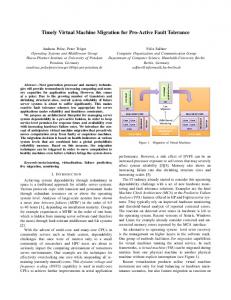
Fig. 1. The MEA cycle of Proactive Fault Management

PFM is based on the Monitor–Evaluate–Act (MEA) cycle, which means that the following three steps are continuously repeated during system runtime: – Monitor. PFM is observation-based, which implies that the system is continuously monitored during its entire operation. Although we will not cover all aspects of monitoring, here, a discussion on aspects such as variable selection and adaptive monitoring is included in Sect. 6. – Evaluate. The monitoring data is continuously evaluated in order to check whether the system’s current state is failure-prone or not. This is the goal of online failure prediction algorithms. Evaluation might also include diagnosis in order to identify the components that cause the system to be failureprone3 . – Act. In case of an imminent failure, counteractions are performed in order to do something about the failure. However, there might be several actions available, such that the most effective method needs to be selected. Effectiveness of actions is evaluated based on an objective function taking cost of actions, confidence in the prediction, probability of success and complexity of actions into account. In addition to selecting an appropriate action, its execution needs to be scheduled, e.g., at times of low system utilization, and it needs to be executed. Our MEA approach is similar to the Monitor, Analyze, Plan, Execute (MAPE) cycle introduced by IBM in the context of autonomic computing and failure prediction [70,40] but we have decided to merge “planning” and “execution” 3

Note that in contrast to traditional diagnosis, in PFM no failure has occurred, yet, posing new challenges for diagnosis algorithms.

174


into one group since for many environments planning and execution are tightly coupled. For example, planning frequently relies on the action selected (e.g., planning of a (partial) restart probably needs to take other constraints into account than moving computations from one server to another). It should also be noted that both loops in fact are control loops, and the general principles of control theory apply to both of them. More specifically, when designing a dependable system, control loop aspects such as stability and the occurrence of oscillations should be checked for any given approach (see [59] for a good example how this can be done). Several examples for systems employing proactive fault management have been described in the literature. In [16] a framework called application cluster service is described that facilitates failover (both preventive and after a failure) and state recovery services. FT-Pro, which is a failure prediction-driven adaptive fault management system, was proposed in [50]. It uses false positive error rate and false negative rate of a failure predictor together with cost and expected downtime to choose among the options to migrate processes, to trigger checkpointing or to do nothing.

3

Online Failure Prediction Methods

Predicting the future has fascinated people from beginning of times. World wide, millions work on prediction daily. Experts on prediction range from fortune tellers and meteorologists to pollsters, stock brokers, doctors and scientists. Predictive technologies have been and are used in a variety of areas and in disaster and failure management they cover a wide range from eliminating minor inconveniences to saving human lives. In a more technical context, failure prediction has a long tradition in mechanical engineering. Especially in the area of preventive maintenance, forecasting a device’s failure has been of great interest, which has been accompanied by reliability theory (See, e.g., [29] for an overview). A key input parameter of these models is the distribution of time to failure. Therefore, a lot of work exists providing methods to fit various reliability models to data with failure time occurrences. There were also approaches that tried to incorporate several factors into the distribution. For example, the MIL-book 217 [57] classified, among others, the manufacturing process whereas several software reliability methods incorporated code complexity, fixing of bugs, etc. into their models (see, e.g., [25]). However, these methods are tailored to long-term predictions and do not work appropriately for short-term predictions (i.e., for the next few minutes to hours) as are needed for the PFM. That is why methods for online failure prediction are based on runtime monitoring in order to take into account the current state of the system. Nevertheless, techniques from classical reliability theory can help to improve online failure prediction as well. A variety of runtime monitoring-based methods have been developed. In this chapter, we describe a classification taxonomy for prediction methods and present two specific approaches from two categories in more detail. The taxonomy and its description is a condensed version of the one described in survey [65].


3.1

175

Main Categories of Prediction Methods

In order to establish a top-level classification of prediction methods, we first analyze the process of how faults turn into failures. Several attempts have been made to get to a precise definition of faults, errors, and failures, among which are [54,3,45,18], [67, Page 22], and most recently [4]. Since the latter seems to have broad acceptance, its definitions are used in this article with some additional extensions and interpretations. – A failure is defined as “an event that occurs when the delivered service deviates from correct service”. The main point here is that a failure refers to misbehavior that can be observed by the user, which can either be a human or another computer system. Things may go wrong inside the system, but as long as it does not result in incorrect output (including the case that there is no output at all) there is no failure. – The situation when “things go wrong” in the system can be formalized as the situation when the system’s state deviates from the correct state, which is called an error. Hence, “an error is the part of the total state of the system that may lead to its subsequent service failure.” – Finally, faults are the adjudged or hypothesized cause of an error – the root cause of an error. In most cases, faults remain dormant for some time and once they become active, they cause an incorrect system state, which is an error. That is why errors are also called “manifestation” of faults. Several classifications of faults have been proposed in the literature among which the distinction between transient, intermittent and permanent faults [67, Page 22] and the fault model by Cristian [19], which has later been extended by Laranjeira, et al. [46] and Barborak, et al. [7], are best known. – The definition of an error implies that the activation of a fault lead to an incorrect state, however, this does not necessarily mean that the system knows about it. In addition to the definitions given by [4], we distinguish between undetected errors and detected errors: An error remains undetected until an error detector identifies the incorrect state. – Besides causing a failure, undetected or detected errors may cause out-ofnorm behavior of system parameters as a side-effect. We call this out-of-norm behavior a symptom 4 . In the context of software aging, symptoms are similar to aging-related errors, as implicitly introduced in [31] and explicitly named in [30]. Figure 2 visualizes how a fault can evolve into a failure. Note that there can be an m-to-n mapping between faults, errors, symptoms, and failures: For example, several faults may result in one single error or one fault may result in several errors. The same holds for errors and failures: Some errors result in a failure some errors do not, and more complicated, some errors only result in a failure under special conditions. As is also indicated in the figure, an undetected 4

This should not be confused with [41], who use the term symptom for the most significant errors within an error group.

176


Fig. 2. Interrelations of faults, errors, symptoms, and failures. Encapsulating boxes show the technique by which the corresponding flaw can be made visible.

error may cause a failure directly or might even be non-distinguishable from it. Furthermore, errors do not necessarily show symptoms. To further clarify the terms fault, error, symptom, and failure, consider a fault-tolerant system with a memory leak in its software. The fault is, e.g., a missing free statement in the source code. However, as long as this part of the software is never executed, the fault remains dormant. Once the piece of code that should free memory is executed, the software enters an incorrect state, i.e., it turns into an error (memory is consumed and never freed although it is not needed anymore). If the amount of unnecessarily allocated memory is sufficiently small, this incorrect state will neither be detected nor will it prevent the system from delivering its intended service (no failure is observable from the outside). Nevertheless, if the piece of code with the memory leak is executed many times, the amount of free memory will slowly decrease in the long run. This out-of-norm behavior of the system parameter “free memory” is a symptom of the error. At some point in time, there might not be enough memory for some memory allocation and the error is detected. However, if it is a fault-tolerant system, the failed memory allocation still does not necessarily lead to a service failure. For example, the operation might be completed by some spare unit. Only if the entire system, as observed from the outside, cannot deliver its service correctly, a failure occurs. Since online failure prediction methods evaluate monitoring data in order to determine whether the current system state is failure-prone or not, the algorithms have to tap observations from the process how a fault evolves into a failure. The gray surrounding boxes in Fig. 2 show the techniques by which each stage can be made visible: 1. In order to identify a fault, testing must be performed. The goal of testing is to identify flaws in a system regardless whether the entity under test is actually used by the system or not. For example, in memory testing, the entire memory is examined even though some areas might never be used.


177

Fig. 3. Coarse-grain classification of online failure prediction techniques. The bottom line represents the exemplary approaches presented in this paper.

2. Undetected errors can be identified by auditing. Auditing describes techniques that check whether the entity under audit is in an incorrect state. For example, memory auditing would inspect used data structures by checksumming. 3. Symptoms, which are side-effects of errors, can be identified by monitoring system parameters such as memory usage, workload, sequence of function calls, etc. An undetected error can be made visible by identifying out-of-norm behavior of the monitored system variable(s). 4. Once an error detector identifies an incorrect state the detected error may become visible by reporting. Reports are written to some logging mechanism such as logfiles or Simple Network Management Protocol (SNMP) messages. 5. Finally, the occurrence of failures can be made visible by tracking mechanisms. Tracking is usually performed from outside the system and includes, for example, sending test requests to the system in order to identify service crashes5 . The taxonomy for online failure prediction algorithms is structured along the five stages of fault capturing. However, fault testing is no option for the purpose of online failure prediction and is hence not included in the taxonomy. This taxonomy is discussed in full detail in [65], and we only introduce its main categories here. Figure 3 shows the simplified taxonomy, which also highlights where the two prediction methods that will be discussed in Sect. 3.2 are located. Failure Prediction Based on Symptom Monitoring. The motivation for analyzing periodically measured system variables such as the amount of free memory in order to identify an imminent failure is the fact that some types of errors affect the system slowly, even before they are detected (this is sometimes referred to as service degradation). A prominent example are memory leaks: due to a leak the amount of free memory is slowly decreasing over time, but, as long as there is still memory available, the error is neither detected nor is a failure 5

This is sometimes called active monitoring.

178


observed. When memory is getting scarce, the computer may first slow down (e.g., due to memory swapping) and only if there is no memory left an error is detected and a failure might result. The key notion of failure prediction based on monitoring data is that errors like memory leaks can be grasped by their sideeffects on the system (symptoms) such as exceptional memory usage, CPU load, disk I/O, or unusual function calls in the system. Symptom-based online failure prediction methods frequently address non-failstop failures, which are usually more difficult to grasp. This group of failure prediction methods comprises the majority of existing prediction techniques. Well-known approaches are the Multivariate State Estimation Technique (MSET) [68], trend analysis techniques like the one developed in [28] or function approximation approaches. The Universal Basis Functions (UBF) failure prediction method, which is described in Sect. 3.2, belongs to this category. Failure Prediction Based on Undetected Error Auditing. Although auditing of undetected errors can be applied offline, the same techniques can be applied during runtime as well. However, we are not aware of any work pursuing this approach, hence the branch has no further subdivisions. Failure Prediction Based on Detected Error Reporting. When an error is detected, the detection event is usually reported using some logging facility. Hence, failure prediction approaches that use error reports as input data have to deal with event-driven input data. This is one of the major differences to symptom monitoring-based approaches, which in most cases operate on periodic system observations. Furthermore, symptoms are in most cases real-valued while error events mostly are discrete, categorical data such as event IDs, component IDs, etc. The problem statement of detected error failure prediction is shown in Fig. 4. Based on error events that have occurred within a data window prior to present time, online failure prediction has to assess whether a failure will occur at some point of time in the future or not. Siewiorek and Swarz [66] state that the first approaches to error detectionbased failure prediction have been proposed by Nassar et al. [56]. These approaches rely on systematic changes in the distribution of error types and on significant increase of error generation rates between crashes. Another method has been developed by Lin and Siewiorek [52], [51] called Dispersion Frame Technique (DFT). A second group of failure prediction approaches comprises data

Fig. 4. Event-based failure prediction


179

Fig. 5. Failure Prediction using UBF

mining techniques. One of the best-known prediction algorithm of this category has been developed at IBM T.J. Watson by Vilalta et al. (see, e.g., [73]). The authors introduce a concept called event sets and apply data-mining techniques to identify sets of events that are indicative of the occurrence of failures. Further methods have briefly been described by Levy et al. in [49]. We have developed a failure prediction method that is based on pattern recognition. More specifically, the main concept is to use hidden semi-Markov models (HSMM) to identify patterns of errors that are symptomatic for an upcoming failure (see Sect. 3.2). Failure Prediction Based on Failure Tracking. The basic idea of failure prediction based on failure tracking is to draw conclusions about upcoming failures from the occurrence of previous failures. This may include the time of occurrence as well as the types of failures that have occurred. Failure predictors of this category have been proposed in, e.g., [20] and [61]. 3.2

Two Exemplary Methods

Two online failure prediction methods have been developed at Computer Architecture and Communication Group at Humboldt University Berlin: UBF and HSMM. The two methods will be described briefly in order to provide a better understanding of how online failure prediction can be accomplished. Both approaches have been applied to a case study, as is described in Sect. 3.3. Universal Basis Functions (UBF). UBF [37] is a function approximation method that takes monitoring variables such as workload, number of semaphore operations per second, and memory consumption as input data. It consists of three steps: First, most indicative variables are selected by the Probabilistic Wrapper Approach (PWA). In a subsequent step recorded training data is analyzed in order to identify UBFs that map the monitoring data onto the target function. The target function can be any failure indicator such as service availability, which was the one chosen in the case study (see Fig. 5). The third step consists of applying UBFs to monitoring data during runtime in order to perform online failure prediction. These steps are usually repeated until a sufficient level of failure prediction accuracy is reached (see [35] for details).

180


PWA is a variable selection algorithm that combines forward selection and backward elimination (c.f., [33]) in a probabilistic framework. It has proven to be very effective, outperforming by far both methods as well as a selection by (human) domain experts [35]. UBF are an extension of Radial Basis Functions (RBF, c.f. [21]). One UBF is a mixture of two kernels used instead of one single Gaussian kernel: ki (x) = mi γ(x, λγi ) + (1 − mi )δ(x, λδi )

(1)

where ki denotes the UBF kernel that is a mixture of kernels γ and δ with parameter vectors λγi and λδi , respectively. Parameter mi is the mixture weight and x is the input vector. By including mi in the optimization, UBF can better adapt to specifics of the data. For example, if a Gaussian and a sigmoid kernel are mixed, either “peaked”, “stepping” or mixed behavior can be modeled in various regions of the input space. Event-based Pattern Recognition using Hidden Semi-Markov Models (HSMM). Taking all errors into account that occur within a time window of length Δtd , error event timestamps and message IDs form an event-driven temporal sequence, which we called error sequence. Based on this notion, the task of failure prediction is turned into a pattern recognition problem where the goal is to identify if the error pattern observed during runtime is indicative for an upcoming failure or not. Hidden semi-Markov models are used as pattern recognition tool and machine learning techniques are applied in order to algorithmically identify characteristic properties indicating whether a given error sequence is failure-prone or not. Of course, error sequences are rarely identical. Therefore, a probabilistic approach is adopted to handle similarity. More specifically, failure and non-failure error sequences are extracted from training data for which it is known when failures had occurred. Failure sequences are error sequences that have occurred preceding a failure by lead time Δtl . Nonfailure sequences consist of errors appearing in the log when no failures have occurred (see Fig. 6). Two HSMMs are trained: One for failure sequences and the other for non-failure sequences. The main goal of training is that the failure HSMM is specifically tailored towards characteristics of failure sequences, and the non-failure HSMM is mainly needed for sequence classification. Once the two models have been trained, new unknown sequences that occur during runtime can be evaluated. For this, sequence likelihood (which is a probabilistic measure of similarity to training sequences) is computed for both HSMM models and Bayes decision theory is applied in order to yield a classification. In other words, by training, the failure model has learned what error sequences look like. Hence, if the sequence under consideration is very similar to failure sequences in the training data (the failure sequence HSMM outputs a higher sequence likelihood than the non-failure HSMM), it is assumed that a failure is looming which will occur at time Δtl ahead. A thorough analysis of the algorithm’s properties such as accuracy of the initial training and complexity aspects together with measurements regarding the computational overhead can be found in [64].


181

Fig. 6. Training hidden semi-Markov models (HSMM) from recorded training sequences. A,B,C denote error events, denote the occurrence of failures, Δtd denotes the length of the data window, Δtl denotes lead time before failure.

3.3

A Case Study

In order to show how well the failure predictors described in the previous sections work for contemporary complex computer systems, we sketch an extensive case study where we applied the UBF and HSMM failure predictors to data of a commercial telecommunication system. The main purpose of the telecommunication system is to realize a so-called Service Control Point (SCP) in an Intelligent Network (IN). An SCP provides services6 to handle communication related management data such as billing, number translations or prepaid functionality for various services of mobile communication: Mobile Originated Calls (MOC), Short Message Service (SMS), or General Packet Radio Service (GPRS). The fact that the system is an SCP implies that the system cooperates closely with other telecommunication systems in the Global System for Mobile Communication (GSM), but the system does not switch calls itself. It rather has to respond to a large variety of different service requests regarding accounts, billing, etc. submitted to the system over various protocols such as Remote Authentication Dial In User Interface (RADIUS), Signaling System Number 7 (SS7), or Internet Protocol (IP). The system’s architecture is a multi-tier architecture employing a componentbased software design. At the time when measurements were taken the system consisted of more than 1.6 million lines of code, approximately 200 components realized by more than 2000 classes, running simultaneously in several containers, each replicated for fault tolerance. Failure Definition and Input Data. As discussed in Sect. 3.1, a failure is defined as the event when a system ceases to fulfill its specification. Specifications for the telecommunication system under investigation require that within successive, non-overlapping five minutes intervals, the fraction of calls having response time longer than 250ms must not exceed 0.01%. This definition is equivalent to a required four-nines interval service availability: Ai = 6

service requests within 5 min. with response time ≤ 250ms total number of service requests within 5 min.

So-called Service Control Functions (SCF).

≥ 99.99%

(2)

182


Hence the failures predicted are performance failures that occur when Eq. 2 does not hold. System error logs and data of the System Activity Reporter (SAR) have been used as input data. Metrics. The quality (i.e., accuracy) of failure predictors is usually assessed by three metrics that have an intuitive interpretation: precision, recall, and false positive rate: – Precision: fraction of correctly predicted failures in comparison to all failure warnings – Recall : fraction of correctly predicted failures in comparison to the total number of failures. Recall is also called true positive rate. – False positive rate: fraction of false alarms in comparison to all non-failures. A perfect failure prediction would achieve a one-to-one matching between predicted and actual failures which would result in precision and recall equal to one and a false positive rate equal to zero. If a prediction algorithm achieves, for example, precision of 0.8, the probability is 80% that any generated failure warning is correct (refers to a true failure) and 20% are false warnings. A recall of, say, 0.9 expresses that 90% of all actual failures are predicted and 10% are missed. A false positive rate of 0.1 indicates that 10% of predictions that should not result in a failure warning are falsely classified as failure-prone. There is often an inverse proportionality between high recall and high precision. Improving recall in most cases lowers precision and vice versa. Many failure predictors (including UBF and HSMM) allow to control this trade-off by use of a threshold. There is also a proportionality between true positive rate (which is equal to recall) and false positive rate: Increasing the true positive rate usually also increases the false positive rate. It is common to visualize this relation by a Receiver-Operating-Characteristic (ROC) [26]. To evaluate and compare failure predictors by a single real number the maximum value of the F-measure (which is the harmonic mean of precision and recall), the value of the point where precision equals recall, or the area under the ROC curve (AUC) can be used. Results. UBF and HSMM have been applied to data collected from the telecommunication system. We report some of the results here in order to give a rough estimate of the accuracy that can be achieved when failure predictors are applied to complex computer systems. For a threshold value that results in maximum F-measure, the HSMM predictor achieves a precision, recall, and false positive rate of 0.70, 0.62, and 0.016, respectively. This means that failure warnings are correct in 70% of all cases and almost two third of all failures are predicted by HSMM. Area under the ROC curve (AUC) equals 0.873. A detailed analysis of HSMM results can be found in [64, Chap. 9]. The UBF approach has been investigated using ROC analysis and achieved an AUC equal to 0.846. A detailed analysis of properties and results can be found in [36].


183

Fig. 7. Classification of actions that can be triggered by failure prediction

4

Prediction-Driven Countermeasures

The third phase in the MEA cycle (c.f. Fig. 1) is to act upon the warning of an upcoming failure. This section gives an overview of the methods that can be triggered by a failure warning. 4.1

Types of Actions

There are five classes of actions that can be performed upon failure prediction, as is shown in the coarse-grained classification in Fig. 7. The two principle goals that prediction-driven actions can target are: – Downtime avoidance (or failure avoidance) aims at circumventing the occurrence of the failure such that the system continues to operate without interruption – Downtime minimization (minimization of the impact of failures) involves downtime, but the goal is to reduce downtime exploiting the knowledge that a failure might be imminent. Each category of techniques will be discussed separately in the following. 4.2

Downtime Avoidance

Downtime avoidance actions try to prevent the occurrence of an imminent failure that has not yet occurred. Three categories of mechanisms can be identified: – State clean-up tries to avoid failures by cleaning up resources. Examples include garbage collection, clearance of queues, correction of corrupt data or elimination of “hung” processes. – Preventive failover techniques perform a preventive switch to some spare hardware or software unit. Several variants of this technique exist, one of which is failure prediction-driven load balancing accomplishing gradual “failover” from a failure-prone to failure-free component. For example, a multiprocessor environment that is able to migrate processes in case of an imminent failure is described in [15]. Current virtualization framework such as XEN7 offers flexible and easy-to-use interfaces to perform migration from one (virtual) machine to another. 7

http://www.xen.org

184


– Lowering the load is a common way to prevent failures. For example, webservers reject connection requests in order not to become overloaded. Within proactive fault management, the number of allowed connections is adaptive and would depend on the assessed risk of failure. 4.3

Downtime Minimization

Repairing the system after failure occurrence is the classical way of failure handling. Detection mechanisms such as coding checks, replication checks, timing checks or plausibility checks trigger the recovery. Within proactive fault management, these actions still incur downtime, but its occurrence is either anticipated or even intended in order to reduce time-to-repair. Two categories exist: – Prepared repair tries to prepare recovery mechanisms for the upcoming failure. Similar to traditional fault tolerance techniques, these methods still react to the occurrence of a failure, but due to preparation, repair time is reduced. – Preventive restart intentionally brings the system down for restart turning unplanned downtime into forced downtime, which is expected to be shorter (fail fast policy). Prepared Repair. The main objective of reactive downtime minimization is to bring the system into a consistent fault-free state. If the fault-free state is a previous one (a so-called checkpoint), the action applies a roll-backward scheme (see, e.g., [24] for a survey of roll-back recovery in message passing systems). In this case, all computation from the last checkpoint up to the time of failure occurrence has to be repeated. Typical examples are recovery from a checkpoint or the recovery block scheme introduced by [62]. In case of a roll-forward scheme, the system is moved to a new fault-free state (see, e.g., [63]). Both schemes may comprise reconfiguration such as switching to a hardware spare or another version of a software program, changing network routing, etc. Reconfiguration takes place before computations are repeated. In traditional fault-tolerant computing without proactive fault management, checkpoints are saved independently of upcoming failures, e.g., periodically. When a failure occurs, first, reconfiguration takes place until the system is ready for recomputation / approximation and then all the computations from the last checkpoint up to the time of failure occurrence are repeated. Time-to-repair (TTR) is determined by two factors: time needed to get a fault-free system by hardware repair or reconfiguration, plus the time needed to redo lost computations (in case of roll-backward) or time to get to a new fault-free state (in case of roll-forward). In the case of roll-backward strategies, recomputation time is determined by the length of the time interval between the checkpoint and the time of failure occurrence. This is illustrated in Fig. 8. In the figure, “Checkpoint” denotes the last checkpoint before failure, “Failure” the time of failure occurrence, “Fault-free” the time when a fault-free system is available and “Up” the time when the system is up again (with a consistent state). In some cases recomputation may take less time than originally but the implication still holds. Note that


185

Fig. 8. Improved time-to-repair for prediction-driven repair schemes. (a) classical recovery and (b) improved recovery in case of preparation for an upcoming failure.

specific reactive downtime minimization techniques do not always exhibit both factors contributing to TTR. Triggering such methods proactively by failure prediction can reduce both factors contributing to TTR: – Time needed to obtain a fault-free system can be reduced since mechanisms can be prepared for an upcoming failure. Think, for example, of a cold spare: Booting the spare machine can be started right after an upcoming failure has been predicted (and hence before failure occurrence) such that a running fault-free system is available earlier after failure. – Checkpoints may be saved upon failure prediction close to the failure, which reduces the amount of computation that needs to be repeated. This minimizes time consumed by recomputation. On the other hand, it might not be wise to save a checkpoint at a time when a failure can be anticipated since the system state might already be corrupted. The question whether such scheme is applicable depends on fault isolation between the system that is going to observe the failure and the state that is included in the checkpoint. For example, if the amount of free memory is monitored for failure prediction but the checkpoint comprises database tables of a separate database server, it might be proper to rely on the correctness of the database checkpoint. Additionally, an adaptive checkpointing scheme similar to the one described in [58] could be applied. In [47] predictive checkpointing for a high-availability high performance Linux cluster has been implemented. Preventive Restart. Parnas [60] has reported on an effect what he called software aging, being a name for effects such as memory leaks, unreleased file locks, accumulated round-off errors, or memory corruption. Based on these observations, Huang et al. introduced a concept that the authors termed rejuvenation. The idea of rejuvenation is to deal with problems related to software aging by restarting the system (or at least parts of it). By this approach, unplanned / unscheduled / unprepared downtime incurred by non-anticipated failures is replaced by forced / scheduled / anticipated downtime. The authors have shown that – under certain assumptions – overall downtime and downtime cost can be reduced by this approach. In [12] the approach is extended by introducing recovery-oriented

186


computing (see, e.g., [10]), where restarting is organized recursively until the problem is solved. In the context of proactive fault management the restart is triggered by failure prediction. Also, a resource consumption trend estimation technique has been implemented into IBM Director Management Software for xSeries servers that can restart parts of the system [14].

5

A Model to Assess the Effect on Reliability

Reliability modeling is an integral part in architecting dependable systems. We have developed a Continuous Time Markov Chain (CTMC) model to assess the effects of proactive fault management on steady-state system availability, reliability and hazard rate. This section introduces the model and lists key results, a full derivation and analysis can be found in [64, Chap. 10]. 5.1

Summary of Proactive Fault Management Behavior

Before introducing the CTMC model for reliability assessment, we summarize the behavior of proactive fault management and its effects on mean-time-to-failure (MTTF) and mean-time-to-repair (MTTR). The behavior can be summarized as follows: If the the evaluation step in the MEA cycle (i.e., failure prediction) suggests that the system is running well and no failure is anticipated in the near future (negative prediction), no action is triggered. If the conclusion is that there is a failure comping up (positive prediction) downtime avoidance methods, downtime minimization methods, or both are triggered. From this follows that in case of a false positive prediction (there is no failure coming up although the predictor suggests so, c.f., Sect. 3.3) actions are performed unnecessarily while in case of a false negative prediction (a failure is imminent but the predictor does not warn about it) nothing is done. Table 1 summarizes all four cases. 5.2

Related Work on Models

Proactive fault management is rooted in preventive maintenance, that has been a research issue for several decades (an overview can be found, e.g., in [29]). More specifically, proactive fault management belongs to the category of conditionbased preventive maintenance (c.f., e.g., [69]). However, the majority of work Table 1. Summary of proactive fault management behavior Prediction

Downtime avoidance

True positive False positive True negative False negative

Try to prevent failure Unneces. action No action No action

Downtime minimization Prepared repair Preventive restart Prepare repair Force downtime Unneces. preparation Unneces. downtime No action No action Standard (unprep.) No action repair (recovery)


187

has been focused on industrial production systems such as heavy assembly line machines and more recently on computing hardware. With respect to software, preventive maintenance has focused more on long-term software product aging such as software versions and updates rather than short-term execution aging. The only exception is software rejuvenation which has been investigated heavily (c.f., e.g., [42]). Starting from general preventive maintenance theory, reliability of conditionbased preventive maintenance is computed in [44]. However, the approach is based on a graphical analysis of so-called total time on test plots of singleton observation variables such as temperature, etc. rendering the approach not appropriate for application to automatic proactive fault management in software systems. An approach better suited to software has been presented by [1]. They use a continuous-time Markov chain (CTMC) to model system deterioration, periodic inspection, preventive maintenance and repair. However, one of the major disadvantages of their approach is that they assume perfect periodic inspection, which does not reflect failure prediction reality. A significant body of work has been published addressing software rejuvenation. Initially, the authors of [39] have used a CTMC in order to compute steadystate availability and expected downtime cost. In order to overcome various limitations of the model, e.g., that constant transition rates are not well-suited to model software aging, several variations to the original model of Huang et al. [39] have been published over the years, some of which are briefly discussed here. Dohi et al. have extended the model to a semi-Markov process to deal more appropriately with the deterministic behavior of periodic restarting. Furthermore, they have slightly altered the topology of the model since they assume that there are cases where a repair does not result in a clean state and restart (rejuvenation) has to be performed after repair. The authors have computed steady-state availability [23] and cost [22] using this model. A slightly different model and the use Weibull distributions to characterize state transitions was proposed in [13]. However, due to this choice, the model cannot be solved analytically and an approximate solution from simulated data is presented. In [27] the authors have used a three state discrete time Markov chain (DTMC) with two subordinated non-homogeneous CTMCs to model rejuvenation in transaction processing systems. One subordinated CTMC models queuing behavior of transaction processing and the second models preventive maintenance. The authors compute steady-state availability, probability of loosing a transaction, and an upper bound on response time for periodic rejuvenation. They model a more complex scheme that starts rejuvenation when the processing queue is empty. The same three-state macro-model has been used in [71], but here, time-to failure is estimated using a monitoring-based subordinated semi-Markov reward model. For model solution, the authors approximate time-to-failure with an increasing failure rate distribution. A detailed stochastic reward net model of a high availability cluster system in order to model availability was presented in [48]. The model differentiates between servers, clients and network. Furthermore, it distinguishes permanent

188


as well as intermittent failures that are either covered (i.e., eliminated by reconfiguration) or uncovered (i.e., eliminated by rebooting the cluster). Again, the model is too complex to be analyzed analytically and hence simulations are performed. An analytical solution for computing the optimal rejuvenation schedule is provided in [2] and uses deterministic function approximation techniques to characterize the relationship between aging factors and work metrics. The optimal rejuvenation schedule can then be found by an analytical solution to an optimization problem. The key property of proactive fault management is that it operates upon failure predictions rather than on a purely time-triggered execution of faulttolerance mechanisms. The authors of [72] propose several stochastic reward nets (SRN), one of which explicitly models prediction-based rejuvenation. However, there are two limitations to this model: first, only one type of wrong predictions is covered, and second, the model is tailored to rejuvenation – downtime avoidance or prepared repair are not included. Furthermore, due to the complexity of the model, no analytical solution for availability is presented. Focusing on service degradation, a CTMC that includes the number of service requests in the system plus the amount of leaked memory was proposed in [6]. An adaptive rejuvenation scheme is analyzed that is based on estimated resource consumption. Later, the model has been combined with the three-state macro model presented in [27] in order to compute availability. In summary, there is no model that incorporates all four types of predictions (TP, FP, TN, FN) and that accounts for the effects of downtime minimization and downtime avoidance methods. The following sections introduce such a model and show how availability, reliability and hazard rate can be computed from it. 5.3

Computing Availability

The model presented here is based on the CTMC originally published by Huang et. al [39]. It differs from their model in the following ways: – Proactive fault management actions operate upon failure prediction rather than periodically. However, predictions can be correct or false. Moreover, it makes a difference whether there really is a failure imminent in the system or not. Hence, the single failure probable state SP in the original model is split into a more fine-grained analysis: According to the four cases of prediction, there is a state for true positive predictions (ST P ), false positive predictions (SF P ), true negative predictions (ST N ) and false negative predictions (SF N ). – In addition to rejuvenation, proactive fault management involves downtime avoidance techniques. That is why there is a transition in our model from the failure probable states ST P and SF P back to the fault-free “up” state S0 . – With respect to downtime minimization, our model comprises prepared repair in addition to preventive restart. In order to account for their effect on time-to-repair, our model has two down states: one for prepared / forced downtime (SR ) and one for unprepared / unplanned downtime (SF ).


189

Fig. 9. Availability model for proactive fault management

Our CTMC model is shown in Fig. 9. In order to better explain the model, consider the following scenario: Starting from the up-state S0 a failure prediction is performed at some point in time. If the predictor comes to the conclusion that a failure is imminent, it is a “positive” prediction and a failure warning is raised. If this is true (something is really going wrong in the system) the prediction is a true positive and a transition into ST P takes place. Due to the warning, some actions are performed in order to either prevent the failure from occurring (downtime avoidance), or to prepare for some forced downtime (downtime minimization). Assuming first that some preventive actions are performed, let PT P := P (failure | true positive prediction)

(3)

denote the probability that the failure occurs despite of preventive actions. Hence, with probability PT P a transition into failure state SR takes place, and with probability (1 − PT P ) the failure can be avoided and the system returns to state S0 . Due to the fact that a failure warning was raised (the prediction was a positive one), preparatory actions have been performed and repair is quicker (on average), such that state S0 is entered with rate rR . If the failure warning is wrong (in truth the system is doing well) the prediction is a false positive (state SF P ). In this case actions are performed unnecessarily. However, although no failure was imminent in the system, there is some risk that a failure is caused by the additional workload for failure prediction and subsequent actions. Hence, let PF P := P (failure | false positive prediction)

(4)

denote that an additional failure is induced. Since there was a failure warning, preparation for an upcoming failure has been carried out and hence the system transits into state SR . In case of a negative prediction (no failure warning is issued) no action is performed. If the judgment of the current situation to be non failure-prone is

190


correct (there is no failure imminent), the prediction is a true negative (state ST N ). In this case, one would expect that nothing happens since no failure is imminent. However, depending on the system, even failure prediction (without subsequent actions) may put additional load onto the system which can lead to a failure although no failure was imminent at the time when the prediction started. Hence there is also some small probability of failure occurrence in the case of a true negative prediction: PT N := P (failure | true negative prediction) .

(5)

Since no failure warning has been issued, the system is not prepared for the failure and hence a transition to state SF rather than SR , takes place. This implies that the transition back to the fault-free state S0 occurs at rate rF , which takes longer (on average). If no additional failure is induced, the system returns to state S0 directly with probability (1 − PT N ). If the predictor does not recognize that something goes wrong in the system but a failure comes up, the prediction is a false negative (state SF N ). Since nothing is done about the failure there is no transition back to the up-state and the model transits to the failure state SF without any preparation. SF N hence represents the state when an unpredicted failure is looming (see [64] for details). The transition rates of the CTMC can be split into four groups: – rT P , rF P , rT N , and rF N denote the rate of true/false positive and negative predictions – rA denotes the action rate, which is determined by the average time from start of the prediction to downtime or to return to the fault-free state. – rR denotes repair rate for forced / prepared downtime – rF denotes repair rate for unplanned downtime Effects of forced downtime / prepared repair on availability, reliability, and hazard rate are gauged by time-to-repair. We hence use a repair time improvement factor k that captures the effectiveness of downtime minimization techniques as mean relative improvement, how much faster the system is up in case of forced downtime / prepared repair in comparison to MTTR after an unanticipated failure: MT T R k= , (6) M T T Rp which is the ratio of MTTR without preparation to MTTR for the forced / prepared case. Obviously, one would expect that preparation for upcoming failures improves MTTR, thus k > 1, but the definition also allows k < 1 corresponding to a change for the worse. All these rates can be determined from precision, recall, false positive rate and a few additional assumptions. Unfortunately, a full derivation of formulas how these rates can be determined goes beyond the scope of this chapter, we refer to [64, Chap. 10]. Steady-state availability is defined as the portion of uptime versus lifetime, which is equivalent to the portion of time, the system is up. In terms of our


191

CTMC model, availability is the portion of probability mass in steady-state assigned to the non-failed states, which are S0 , ST P , SF P , ST N , and SF N . In order to simplify representation, numbers 0 to 6 (as indicated in Fig. 9) are used to identify the states of the CTMC. Steady-state availability is determined by the portion of time the stochastic process stays in one of the up-states 0 to 4: A=

4

πi = 1 − π5 − π6

(7)

i=0

where πi denotes the steady-state probability of the process being in state i. πi can be determined by algebraically solving the global balance equations of the CTMC (see, e.g., [43]). We hence obtain a closed-form solution for steady-state availability of systems with PFM: A= 5.4

(rA + rp )k rF . k rF (rA + rp ) + rA (PF P rF P + PT P rT P + k PT N rT N + k rF N )

(8)

Computing Reliability and Hazard Rate

Reliability R(t) is defined as the probability of failure occurrence up to time t given that the system is fully operational at t = 0. In terms of CTMC modeling this is equivalent to a non-repairable system and computation of the first passage time into a down-state. Therefore the CTMC model shown in Fig.9 can be simplified: the distinction between two down-states (SR and SF ) is not required anymore and there’s no transition back to the up-state. The distribution of the probability to first reach the down-state SF yields the cumulative distribution of time-to-failure. In terms of CTMCs this quantity is called first-passage-time distribution F (t). Reliability R(t) and hazard rate h(t) can be computed from F (t) in the following way: R(t) = 1 − F (t) f (t) , h(t) = 1 − F (t)

(9) (10)

where f (t) denotes the corresponding probability density of F (t). In our model F (t) and f (t) are the cumulative and density of a phase-type exponential distribution defined by T and t0 (see, e.g., [43]): F (t) = 1 − α exp (t T ) e

(11)

f (t) = α exp (t T ) t0 ,

(12)

where e is a vector with all ones, exp (t T ) denotes the exponential of matrix T , which is a sub-matrix of the generator matrix, and α is the initial state probability distribution, which is equal to: α = [1

0 0

0 0] .

(13)

192


Closed form expressions exist and can be computed using a symbolic computer algebra tool. However, the solution would fill several pages8 and will hence not be provided here. 5.5

An Example

In order to give an example, we computed availability and plotted the reliability and hazard rate functions. For the parameters we used the values from HSMMbased failure prediction applied to the telecommunication system (see Sect. 3.3). Since we could not apply countermeasures in the commercial system, we assumed reasonable and moderate values for for PT P , PF P , PT N , and k (see Tab. 2). Table 2. Parameters assumed in the example

1.0

recall 0.62

PT P 0.25

fpr 0.016

PF P 0.1

PT N 0.001

k 2

8e−05

precision 0.70

Parameter Value

with PFM w/o PFM

h(t) 0.0

0e+00

0.2

2e−05

0.4

4e−05

R(t)

0.6

6e−05

0.8

w/o PFM with PFM

0

10000

20000

30000

40000

50000

0

time [s]

200

400

600

800

1000

time [s]

(a)

(b)

Fig. 10. Plots of (a) reliability and (b) hazard rate for the example

The effect on availability can best be seen from the ratio of unavailability with PFM to unavailability without PFM: 1 − AP F M ≈ 0.488 . 1−A

(14)

where AP F M denotes steady-state system availability with proactive fault management, computed from Eq. 8, and A denotes steady-state system availability of a system without PFM computed from a simple CTMC with two states (up and down) and the same failure and repair rates as for the case with PFM. The analysis shows that unavailability is roughly cut down by half. Reliability and hazard rate are also significantly improved, as can be seen from Fig. 10. 8

The solution found by Maplecontains approximately 3000 terms.


6

193

Architectural Blueprint

Incorporating proactive fault management into a system architecture is not a simple task due to various reasons: – It requires spelled out objectives and constraints, both from a business as well as from a technical perspective. – It requires input data from all architectural levels. – It requires domain experts at all architectural levels to identify appropriate failure prediction algorithms as well as available countermeasures. – It requires thorough modeling and analysis at all levels. – Maintenance and development of the proactive fault management modules have to be tightly coupled with the development process of the controlled system. Figure 11 shows an architectural blueprint for a system with proactive fault management. As can be seen, we propose to have separate failure predictors for each system layer. That is, we propose to set up several failure predictors, each analyzing the monitoring data of its specific layer. Such approach enables to develop failure prediction algorithms that are tailored to the specifics of its layer: It allows to select algorithms that are appropriate in terms of specific properties of the input data and allow to handle the amount of data incurred. For example, a predictor on hardware level has to process a large amount of data but failure patterns are not extremely complex, whereas an application level predictor might employ complex pattern recognition algorithms in order to capture failure-prone system states on application level. System level failure predictors cannot operate independently. For illustration just imagine that both a hardware level failure predictor as well as a Virtual Machine Monitor (VMM) level failure predictor predict an upcoming failure. If the two predictors would operate independently, the VMM failure predictor could trigger the migration of a virtual machine from one physical CPU to another and the hardware level failure predictor would restart the CPU at the same time

Fig. 11. An architecture for a system with proactive fault management

194


migration is taking place. For this reason we propose to have the “Act” component of the MEA cycle span all system layers: It incorporates the predictions of its level predictors in order to select the most appropriate countermeasure. In order to do so, we propose to apply techniques known as meta-learning. A survey on meta-learning can be found in [74]. One of the best-known meta-learning algorithms is called “stacked generalization” [34], which has successfully been applied to predict failures for the IBM Blue Gene /L Systems [32]. The decision which countermeasure to apply should not only depend on the output of the domain failure predictors but has to take other factors into account: – Treatment of dependent failures. This involves, for example, that a history of identified faults and the countermeasures taken need to be kept. Another solution might involve the determination of dependencies in the system, such as performed in [11]. – Probabilities of success and the costs involved. Depending on the situation, some countermeasures are more likely to solve the underlying problem than others. The same holds for the costs involved: a slight performance degradation is probably less expensive than a restart of the entire system. The decision, which countermeasure to choose must take these factors into account. – In addition to the direct costs mentioned before, there might also be boundary business constraints and objectives. For example, if the business has service contracts with one company that offers one maintenance operation per month for free, it might in some cases be actually cheaper to rely on manual repair rather than automated proactive fault management. – In case of limited budget, tough choices have to be made and we need to find out at which level we will achieve the highest payoff in terms of dependability gain with minimum performance degradation when PFM methods are used. We call such a desirable system property translucency which means that we have an insight into dependability and performance at all levels while applying specific MEA methods. We mentioned in the introduction that today’s systems are highly dynamic. This is a challenge for implementing proactive fault management. First, if system behavior changes frequently (due to frequent updates and upgrades), the failure prediction approaches have to be adopted to the changed behavior, too. For example, if the prediction algorithm’s parameters have been determined from training data using machine learning techniques, it might be necessary to repeat parameter determination. Online change point detection algorithms such as [8] can be used to determine whether the parameters have to be re-adjusted. A second critical aspect of system dynamicity is that the capabilities belonging to proactive fault management need to be kept in sync with the functional capabilities of the servicing system. Since development frequently is driven by features, the software engineering processes governing proactive fault management have to be adapted accordingly. This also involves thorough modeling and analysis of the entire MEA cycle. Since the MEA cycle forms a control loop in the sense of classical control theory, it can be helpful to apply methods from control theory (such as has been performed in [59]).


195

Last but not least, dynamicity requires new approaches to monitoring: In an environment where components from various vendors appear and disappear, a robust and flexible monitoring infrastructure is required. Such infrastructure must be pluggable such that new monitoring data sources can be incorporated easily. A second requirement are standardized data formats (such as the Common Base Event Model [9]). Furthermore, monitoring should be adaptable during runtime. Failure predictors performing variable selection during runtime should be able to adapt, e.g., the frequency or precision of the data for a monitored object. For example, if a failure predictor identifies, that simply taking the mean over a fixed time interval is not sufficient for accurate predictions, it should be able to adjust monitoring on-the-fly.

7

Conclusions and Research Issues

As computer and communication systems continue to be more complex, it goes without saying that proactive fault management plays and will continue to play an ever more significant role. Traditional methods already fail to cope with complexity at industrial level and they are inadequate to model the systems’ behavior due to dynamicity (frequent changes in configuration, updates, upgrades, extensions and patches) and rapid proliferation in numerous application domains. So the main reasonable approach, in addition to all methods to date, is the use of PFM where with help of predictive technologies downtime can be effectively eliminated by failure avoidance or minimized by efficient preparation for anticipated failures. This can be done by the methods introduced in this paper in combination with effective recovery techniques. System dynamics, changing environments and diverse user preferences will only magnify the usefulness and power of PFM provided a comprehensive system translucency is supported at the design time and architectural trade-offs are well understood at every design layer. Massive redundancy, robust operating systems, composability and self-* (autonomic) computing will effectively complement the PFM methods to further enhance dependability of the future systems. In fact, there is a realistic potential to significantly increase availability as it is predicted from our CTMC model. There is still a number of requirements and research issues that need to be tackled. First of all more field data for reference and benchmarking purposes is needed but it is very difficult to make it available to the research community. Most companies do not like to share the data and the “anonymization” efforts have not been successful despite interest from various companies [53] . Field data need to be conditioned to be used for effective prediction experiments and it usually takes an enormous amount of effort. Only a concerted effort of industry and academia can solve this issue. Also, bridging the gap between academic approaches and industry will help to assess the use of such methods in widely distributed environments. There are some at cost accessible databases such as RIAC9 and other sources supported by Reliasoft10 but they are of little use to 9 10

http://www.theriac.org/ http://www.reliasoft.com/predict/features2.htm

196


academic community. Therefore, the academic/industrial efforts such as AMBER (Assessing, Measuring and Benchmarking Resilience)11 and USENIX12 to collect failure rates and traces are highly commendable and are gaining critical mass to be useful to a broad research community. One of the interesting outcomes from the work on the UBF method was that the focus on variable selection has a major impact on model quality. It is important to find out how sensitive are prediction methods to system changes such as reconfiguration, updates, extensions, etc. Adaptive, self-learning methods need to be developed that are able to minimize or even bypass training and tuning and adjust themselves to new system conditions. The objective function to find out what are the optimal reaction schemes in view of a looming failure is an open research issue. Many practitioners would also like to know the root cause of a looming or actual failure. The research on this topic goes on and some online root cause analysis are under investigation. The trade-offs between workload profile, fault coverage, prediction processing time, prediction horizon and prediction accuracy must also further be researched in order to transfer the PFM methods into engineering practice of architecting dependable systems.

References 1. Amari, S.V., McLaughlin, L.: Optimal design of a condition-based maintenance model. In: Proceedings of Reliability and Maintainability Symposium (RAMS), pp. 528–533 (January 2004) 2. Andrzejak, A., Silva, L.: Deterministic models of software aging and optimal rejuvenation schedules. In: Proceedings of 10th IEEE/IFIP International Symposium on Integrated Network Management (IM 2007), pp. 159–168 (May 2007) 3. Aviˇzienis, A., Laprie, J.-C.: Dependable computing: From concepts to design diversity. Proceedings of the IEEE 74(5), 629–638 (1986) 4. Algirdas Aviˇzienis, J.-C., Laprie, B., Randell, B., Landwehr, C.: Basic concepts and taxonomy of dependable and secure computing. IEEE Transactions on Dependable and Secure Computing 1(1), 11–33 (2004) 5. Babaoglu, O., Jelasity, M., Montresor, A., Fetzer, C., Leonardi, S., van Moorsel, A., van Steen, M. (eds.): SELF-STAR 2004. LNCS, vol. 3460. Springer, Heidelberg (2005) 6. Bao, Y., Sun, X., Trivedi, K.S.: Adaptive software rejuvenation: Degradation model and rejuvenation scheme. In: Proceedings of the 2003 International Conference on Dependable Systems and Networks (DSN 2003). IEEE Computer Society, Los Alamitos (2003) 7. Barborak, M., Dahbura, A., Malek, M.: The Consensus Problem in Fault-Tolerant Computing. Computing Surveys (CSUR) 25(2), 171–220 (1993) 8. Basseville, M., Nikiforov, I.V.: Detection of abrupt changes: theory and application. Prentice Hall, Englewood Cliffs (1993) 9. Bridgewater, D.: Standardize Messages with the Common Base Event Model (2004), http://www-106.ibm.com/developerworks/autonomic/library/ac-cbe1/ 11 12

http://www.amber-project.eu/ http://cfdr.usenix.org/


197

10. Brown, A., Patterson, D.A.: Embracing failure: A case for recovery-oriented computing (roc). In: High Performance Transaction Processing Symposium (October 2001) 11. Candea, G., Delgado, M., Chen, M., Fox, A.: Automatic Failure-Path Inference: A Generic Introspection Technique for Internet Applications. In: Proceedings of 3rd IEEE Workshop on Internet Applications (WIAPP), San Jose, CA (June 2003) 12. Candea, G., Cutler, J., Fox, A.: Improving availability with recursive microreboots: A soft-state system case study. Performance Evaluation Journal 56(1-3) (March 2004) 13. Cassady, C.R., Maillart, L.M., Bowden, R.O., Smith, B.K.: Characterization of optimal age-replacement policies. In: IEEE Proceedings of Reliability and Maintainability Symposium, pp. 170–175 (January 1998) 14. Castelli, V., Harper, R.E., Heidelberger, P., Hunter, S.W., Trivedi, K.S., Vaidyanathan, K., Zeggert, W.P.: Proactive management of software aging. IBM Journal of Research and Development 45(2), 311–332 (2001) 15. Chakravorty, S., Mendes, C., Kale, L.V.: Proactive fault tolerance in large systems. In: HPCRI Workshop in conjunction with HPCA 2005 (2005) 16. Cheng, F.T., Wu, S.L., Tsai, P.Y., Chung, Y.T., Yang, H.C.: Application cluster service scheme for near-zero-downtime services. In: IEEE Proceedings of the International Conference on Robotics and Automation, pp. 4062–4067 (2005) 17. Coleman, D., Thompson, C.: Model Based Automation and Management for the Adaptive Enterprise. In: Proceedings of 12th Annual Workshop of HP OpenView University Association, pp. 171–184 (2005) 18. International Electrotechnical Commission. Dependability and quality of service. In IEC: International Technical Comission, editor, IEC 60050: International Electrotechnical Vocabulary, IEC, 2 edn. ch. 191 (2002) 19. Cristian, F., Aghili, H., Strong, R., Dolev, D.: Atomic Broadcast: From Simple Message Diffusion to Byzantine Agreement. In: Proceedings of 15th International Symposium on Fault Tolerant Computing (FTCS). IEEE, Los Alamitos (1985) 20. Csenki, A.: Bayes predictive analysis of a fundamental software reliability model. IEEE Transactions on Reliability 39(2), 177–183 (1990) 21. Buhmann, M.D.: Radial basis functions: theory and implementations. Cambridge monographs on applied and computational mathematics, vol. 12. Cambridge University Press, Cambridge (2003) 22. Dohi, T., Goseva-Popstojanova, K., Trivedi, K.S.: Analysis of software cost models with rejuvenation. In: Proceedings of IEEE Intl. Symposium on High Assurance Systems Engineering, HASE 2000 ( November 2000) 23. Dohi, T., Goseva-Popstojanova, K., Trivedi, K.S.: Statistical non-parametric algorihms to estimate the optimal software rejuvenation schedule. In: Proceedings of the Pacific Rim International Symposium on Dependable Computing, PRDC 2000 (December 2000) 24. Elnozahy, E.N., Alvisi, L., Wang, Y., Johnson, D.B.: A survey of rollback-recovery protocols in message-passing systems. ACM Computing Surveys 34(3), 375–408 (2002) 25. Farr, W.: Software reliability modeling survey. In: Lyu, M.R. (ed.) Handbook of software reliability engineering, ch. 3, pp. 71–117. McGraw-Hill, New York (1996) 26. Flach, P.A.: The geometry of ROC space: understanding machine learning metrics through ROC isometrics. In: Proceedings of 20th International Conference on Machine Learning (ICML 2003), pp. 194–201. AAAI Press, Menlo Park (2003) 27. Garg, S., Puliafito, A., Telek, M., Trivedi, K.S.: Analysis of preventive maintenance in transactions based software systems. IEEE Trans. Comput. 47(1), 96–107 (1998)

198


28. Garg, S., van Moorsel, A., Vaidyanathan, K., Trivedi, K.S.: A methodology for detection and estimation of software aging. In: Proceedings of the 9th International Symposium on Software Reliability Engineering, ISSRE (Novomber 1998) 29. Gertsbakh, I.: Reliability Theory: with Applications to Preventive Maintenance. Springer, Berlin (2000) 30. Grottke, M., Matias, R., Trivedi, K.S.: The Fundamentals of Software Aging. In: Proceedings of Workshop on Software Aging and Rejuvenation, in conjunction with ISSRE, Seattle, WA. IEEE, Los Alamitos (2008) 31. Grottke, M., Trivedi, K.S.: Fighting Bugs: Remove, Retry, Replicate, and Rejuvenate. Computer 40(2), 107–109 (2007) 32. Gujrati, P., Li, Y., Lan, Z., Thakur, R., White, J.: A Meta-Learning Failure Predictor for Blue Gene/L Systems. In: Proceedings of International Conference on Parallel Processing (ICPP 2007). IEEE, Los Alamitos (2007) 33. Guyon, I., Elisseeff, A.: An Introduction to Variable and Feature Selection. Journal of Machine Learning Research 3, 1157–1182 (2003); Special Issue on Variable and Feature Selection 34. Wolpert, D.H.: Stacked Generalization. Neural Networks 5(5), 241–259 (1992) 35. Hoffmann, G.A., Trivedi, K.S., Malek, M.: A Best Practice Guide to Resource Forecasting for Computing Systems. IEEE Transactions on Reliability 56(4), 615– 628 (2007) 36. Hoffmann, G.A.: Failure Prediction in Complex Computer Systems: A Probabilistic Approach. Shaker, Aachen (2006) 37. Hoffmann, G.A., Malek, M.: Call availability prediction in a telecommunication system: A data driven empirical approach. In: Proceedings of the 25th IEEE Symposium on Reliable Distributed Systems (SRDS 2006), Leeds, United Kingdom (October 2006) 38. Horn, P.: Autonomic Computing: IBM’s perspective on the State of Information Technology (October 2001), http://www.research.ibm.com/autonomic/ manifesto/autonomic_computing.pdf 39. Huang, Y., Kintala, C., Kolettis, N., Fulton, N.: Software rejuvenation: Analysis, module and applications. In: Proceedings of IEEE Intl. Symposium on Fault Tolerant Computing, FTCS 25 (1995) 40. IBM. An architectural blueprint for autonomic computing. White paper (June 2006), http://www-01.ibm.com/software/tivoli/autonomic/pdfs/AC_Blueprint_ White_Paper_4th.pdf 41. Iyer, R.K., Young, L.T., Sridhar, V.: Recognition of error symptoms in large systems. In: Proceedings of 1986 ACM Fall Joint Computer Conference, Dallas, Texas, United States, pp. 797–806. IEEE Computer Society Press, Los Alamitos (1986) 42. Kajko-Mattson, M.: Can we learn anything from hardware preventive maintenance? In: Proceedings of the Seventh International Conference on Engineering of Complex Computer Systems, ICECCS 2001, pp. 106–111. IEEE Computer Society Press, Los Alamitos (2001) 43. Kulkarni, V.G.: Modeling and Analysis of Stochastic Systems, 1st edn. Chapman and Hall, London (1995) 44. Kumar, D., Westberg, U.: Maintenance scheduling under age replacement policy using proportional hazards model and ttt-plotting. European Journal of Operational Research 99(3), 507–515 (1997) 45. Laprie, J.-C., Kanoun, K.: Software Reliability and System Reliability. In: Lyu, M.R. (ed.) Handbook of software reliability engineering, pp. 27–69. McGraw-Hill, New York (1996)


199

46. Laranjeira, L.A., Malek, M., Jenevein, R.: On tolerating faults in naturally redundant algorithms. In: Proceedings of Tenth Symposium on Reliable Distributed Systems (SRDS), pp. 118–127. IEEE Computer Society Press, Los Alamitos (September 1991) 47. Leangsuksun, C., Liu, T., Rao, T., Scott, S.L., Libby, R.: A failure predictive and policy-based high availability strategy for linux high performance computing cluster. In: The 5th LCI International Conference on Linux Clusters: The HPC Revolution, pp. 18–20 (2004) 48. Leangsuksun, C., Shen, L., Liu, T., Song, H., Scott, S.L.: Availability prediction and modeling of high mobility oscar cluster. In: IEEE Proceedings of International Conference on Cluster Computing, pp. 380–386 (2003) 49. Levy, D., Chillarege, R.: Early warning of failures through alarm analysis - a case study in telecom voice mail systems. In: Proceedings of the 14th International Symposium on Software Reliability Engineering, ISSRE 2003, Washington, DC, USA. IEEE Computer Society, Los Alamitos (2003) 50. Li, Y., Lan, Z.: Exploit failure prediction for adaptive fault-tolerance in cluster computing. In: IEEE Proceedings of the Sixth International Symposium on Cluster Computing and the Grid (CCGRID 2006), pp. 531–538. IEEE Computer Society, Los Alamitos (2006) 51. Linand, T.-T.Y., Siewiorek, D.P.: Error log analysis: statistical modeling and heuristic trend analysis. IEEE Transactions on Reliability 39(4), 419–432 (1990) 52. Lin, T.-T.Y.: Design and evaluation of an on-line predictive diagnostic system. Master’s thesis, Department of Electrical and Computer Engineering, CarnegieMellon University, Pittsburgh, PA (April 1988) 53. Malek, M., Cotroneo, D., Kalbarczyk, Z., Madeira, H., Penkler, D., Reitenspiess, M.: search of real data on faults, errors and failures,Panel discussion at Sixth European Dependable Computing Conference (EDCC) (October 2006) 54. Melliar-Smith, P.M., Randell, B.: Software reliability: The role of programmed exception handling. SIGPLAN Not. 12(3), 95–100 (1977) 55. Mundie, C., de Vries, P., Haynes, P., Corwine, M.: Trustworthy Computing. Technical report, 10 (2002), http://download.microsoft.com/download/a/f/2/ af22fd56-7f19-47aa-8167-4b1d73cd3c57/twc_mundie.doc 56. Nassar, F.A., Andrews, D.M.: A methodology for analysis of failure prediction data. In: IEEE Real-Time Systems Symposium, pp. 160–166 (1985) 57. Department of Defense. MIL-HDBK-217F Reliability Prediction of Electronic Equipment. Washington D.C (1990) 58. Oliner, A., Sahoo, R.: Evaluating cooperative checkpointing for supercomputing systems. In: IEEE Proceedings of 20th International Parallel and Distributed Processing Symposium, IPDPS 2006 (April 2006) 59. Parekh, S., Gandhi, N., Hellerstein, J., Tilbury, D., Jayram, T.S., Bigus, J.: Using Control Theory to Achieve Service Level Objectives In Performance Management. Real-Time Systems 23(1), 127–141 (2002) 60. Parnas, D.L.: Software aging. In: IEEE Proceedings of the 16th International Conference on Software Engineering (ICSE 1994), pp. 279–287. IEEE Computer Society Press, Los Alamitos (1994) 61. Pfefferman, J.D., Cernuschi-Frias, B.: A nonparametric nonstationary procedure for failure prediction. IEEE Transactions on Reliability 51(4), 434–442 (2002) 62. Randell, B.: System structure for software fault tolerance. IEEE Transactions on Software Engineering 1(2), 220–232 (1975) 63. Randell, B., Lee, P., Treleaven, P.C.: Reliability issues in computing system design. ACM Computing Survey 10(2), 123–165 (1978)

200


64. Salfner, F.: Event-based Failure Prediction: An Extended Hidden Markov Model Approach. Dissertation.de Verlag im Internet, Berlin, Germany (2008) 65. Salfner, F., Lenk, M., Malek, M.: A Survey of Online Failure Prediction Methods. ACM Computing Surveys (CSUR) 42(3), 1–42 (2010) 66. Siewiorek, D.P., Swarz, R.S.: Reliable Computer Systems, 2nd edn. Digital Press, Bedford (1992) 67. Siewiorek, D.P., Swarz, R.S.: Reliable Computer Systems, 3rd edn., p. 908. A. K. Peters, Wellesley (1998) 68. Singer, R.M., Gross, K.C., Herzog, J.P., King, R.W., Wegerich, S.: Model-Based Nuclear Power Plant Monitoring and Fault Detection: Theoretical Foundations. In: Proceedings of Intelligent System Application to Power Systems (ISAP 1997), Seoul, Korea, pp. 60–65 (July 1997) 69. Starr, A.G.: A structured approach to the selection of condition based maintenance. In IEEE Proceedings of Fifth International Conference on Factory 2000 - The Technology Exploitation Process, pages Condition based maintenance (CBM) triggers maintenance activity on a parameter which is indicative of machine health. Regular tasks, which are the staple of planned preventive maintenance become scheduled inspections and measurements rather than repair or (April 1997) 70. Sterritt, R., Parashar, M., Tianfield, H., Unland, R.: A concise introduction to autonomic computing. Advanced Engineering Informatics (AEI) 19(3), 181–187 (2005); Autonomic Computing 71. Vaidyanathan, K., Trivedi, K.S.: A comprehensive model for software rejuvenation. IEEE Transactions on Dependable and Secure Computing 2, 124–137 (2005) 72. Vaidyanathan, K., Harper, R.E., Hunter, S.W., Trivedi, K.S.: Analysis and implementation of software rejuvenation in cluster systems. In: Proceedings of the 2001 ACM SIGMETRICS International Conference on Measurement and Modeling of Computer Systems, pp. 62–71. ACM Press, New York (2001) 73. Vilalta, R., Apte, C.V., Hellerstein, J.L., Ma, S., Weiss, S.M.: Predictive algorithms in the management of computer systems. IBM Systems Journal 41(3), 461–474 (2002) 74. Vilalta, R., Drissi, Y.: A perspective view and survey of meta-learning. Artificial Intelligence Review 18(2), 77–95 (2002)

Architecting Dependable Systems with Proactive Fault ... - CiteMaster

Architecting Dependable Systems with Proactive Fault ... - CiteMaster

Suggest Documents

Architecting Dependable Systems Using Virtualization - CiteSeerX

ICSE 2002 Workshop on Architecting Dependable Systems

Workshop on Architecting Dependable Systems - Semantic Scholar

Architecting Fault-tolerant Component-based Systems: from ...

Architecting Fault Tolerance with Exception ... - Semantic Scholar

Proactive Network Fault Detection

A Fault Injection Method for Testing Dependable Web Service Systems

Byzantine fault tolerance can be fast - Dependable Systems ... - Microsoft

Dependable Fastening Systems

Proactive Network Fault Detection - CiteSeerX

Service Availability of Systems with Failure Prevention - CiteMaster

A Proactive Fault Tolerance Scheme for Large Scale Storage Systems

Dependable Systems Case Studies

Dependable Pervasive Systems - DIRC

Comprehensive Logfiles for Autonomic Systems - CiteMaster

Architecting Systems with Trustworthy Components - DROPS

Architecting Systems with Trustworthy Components - DROPS

Timely Virtual Machine Migration for Pro-Active Fault ... - CiteMaster

Architecting Fault Tolerance with Exception Handling: Verification and ...

Proactive Byzantine Quorum Systems

Dependable e-learning systems

Proactive Fault Tolerance for HPC with Xen Virtualization - Computer ...

Workshop on Dependable Systems of Systems

DEPENDABLE COMPUTING SYSTEMS: Paradigms ... - CiteSeerX