vision systems incorporating the rectification preprocessing step. Finally, the authors in [8] provided designs of an algo- rithm based on census transform in three ...
ARCHITECTURE AND IMPLEMENTATION OF REAL-TIME 3D STEREO VISION ON A XILINX FPGA Sotiris Thomas
Kyprianos Papadimitriou
Apostolos Dollas
Department of Electronic and Computer Engineering Technical University of Crete GR73100 Chania, Greece ABSTRACT Many applications from autonomous vehicles to surveillance can benefit from real-time 3D stereo vision. In the present work we describe a 3D stereo vision design and its implementation that exploits effectively the resources of a Xilinx Virtex-5 FPGA. The post place-and-route design achieved a processing rate of 87 frames per sec (fps) for 1920 × 1200 resolution. The hardware prototype system was tested and validated for several data sets with resolutions up to 400 × 320 and we achieved a processing rate of 1570 fps. 1
Introduction
The purpose of stereo vision algorithms is to construct an accurate depth map out of two or more images of the same scene, taken under a slightly different angle/position. In a set of two images one of them has the role of the reference image while the other is the non-reference one. The basic problem of finding pairs of pixels, one in the reference image and the other in the non-reference image, that correspond to the same point in space, is known as the correspondence problem and has been studied for many decades [1]. The difference in coordinates of the corresponding pixels (or similar features in the two stereo images) is the disparity. Based on the disparity between corresponding pixels and on stereo camera parameters such as the distance between the two cameras and their focal length, one can extract the depth of the related point in space by triangulation. This problem has been widely researched by the computer vision community and appears not only in stereo vision but in other image processing topics as well such as optical flow calculation [2]. The algorithm we study falls into the broad local category producing dense stereo maps. An extensive taxonomy of dense stereo vision algorithms is available in [3], and an online constantly renewed comparison can be found in [4], containing mainly software implementations. In general, the algorithm searches for pixel matches in an area around the reference pixel in the non-reference frame. This entails a heavy processing task as for each pixel the 2D search space should be exhaustively explored. To reduce the search space the epipolar line constraint is applied to reduce the 2D area search space to a 1D line. In the present work we assume that images are rectified prior to processing. Our contributions are: • the way the design of each stage is facilitated by the FPGA structure and its primitive resources;
• a placed-and-routed design allowing real-time processing up to 87 fps for full HD 1920×1200 frames in a mediumend FPGA; • a design modification which improved by 1.6x the system performance. The paper is organized as follows: Section 2 discusses previous work focusing mainly on hardware-related studies. Section 3 describes the algorithm and its individual steps. Section 4 analyses the benefits of mapping the algorithm to an FPGA. An in-depth discussion of our system is given in Section 5. Section 6 has the system performance, and Section 7 discusses future research. 2
Relevant Research
There is ongoing effort by the research community to support real-time processing of 3D stereo vision, in which a rate of 30 fps is desirable for the human eye. Table 1 consolidates representative implementations in different technologies, with information on the maximum resolution and processing rate.
Table 1. Implementation of 3D Stereo Vision in different technologies. Ref [5] [6] [7] [8] [9] [10] [11]
Resolution 160 × 120 320 × 240 320 × 240 320 × 240 640 × 480 640 × 480 1920 × 1080
Disparity 32 20 16 16 128 64 300
fps 30 150 75 574 30 230 30
Technology DSP Spartan-3 Virtex-II GPU 4 Stratix S80 Virtex-4 Spartan-6
Year 1997 2007 2010 2010 2006 2010 2011
The work in [5] was one of the earliest ones to combine the development of cost calculation with the Laplacian of Gaussian in a DSP. More recently, several works developed different algorithms in fully functional FPGA-based systems ranging from relatively simple [6, 7] to more complex ones [9, 10, 11]. The authors of [10, 11] have designed full stereo vision systems incorporating the rectification preprocessing step. Finally, the authors in [8] provided designs of an algorithm based on census transform in three different technologies, i.e. CPU, GPU and DSP; the maximum performance was obtained with the GPU.
3
The Algorithm
In general, a local algorithm matches pixels in the image pair corresponding to the same point on the scene, by computing matching costs between a pixel in the reference frame and a set of pixels in the target frame and selecting the match with the minimum cost. This is known as the Winner-TakeAll (WTA) strategy according to which the algorithm selects the match with the global minimum cost in the search space. Essentially, this process is equivalent to computing a 3D cost matrix (called Disparity Search Image or DSI, shown in Figure 1) of size W ×H ×Dmax , - where W the frame width, H the frame height and Dmax the size of the search space - and selecting the index of the minimum in the Dmax dimension. To improve the results, usually a cost aggregation step that acts on the DSI is interjected between the cost computing and match selecting steps. Post-processing steps can further refine the resulting disparity map.
Fig. 1. Disparity Search Image (DSI) volume. Our algorithm consists of the cost computation step implemented by the Absolute Difference (AD) census combination matching cost, a simple fixed window aggregation scheme, a left/right consistency check and a scan-line belief propagation solution as a post processing step. The AD measure is defined as the absolute difference between two pixels, CAD = |p1 − p2 |, while census [12] is a window based cost that assigns a bit-string to a pixel and is defined as the sum of the Hamming distance between the bit-strings of two pixels. Let Wc be the size of the census window. A pixel’s bit-string is of size Wc2 − 1 and is constructed by assigning 1 if pi > pc or 0 otherwise, for pi ∈ W indow, and pc the central pixel of the window. The two costs are fused by a truncated normalized sum: C(pR , pT ) = max(
CCensus (pR , pT ) CAD (pR , pT ) + , λtrunc ) (1) M ax M ax CAD CCensus
where λtrunc is the truncation value given as parameter. This matching cost encompasses image local light structure (census) as well as information about the light itself (AD), and produces better results than its parts alone, as was shown in [13]. At object borders, the aggregation window necessarily includes costs belonging to two or more objects in the scene, whereas ideally we would like to aggregate only costs of one object. For this reason, truncating the costs to a maximum value helps at least limiting the effect of any outliers in each aggregation window [3].
Fig. 2. Example of 3x3 fixed window aggregation of DSI costs. After initializing the DSI volume with AD-Census costs, we perform a simple fixed window aggregation on the W × H slices of the DSI, illustrated in Figure 2. This is based on the assumption that neighbouring pixels (i.e. pixels belonging in the same window) most likely share the same disparity (depth) as well. Although this does not stand for object borders and slanted surfaces, it produces good results. On the other hand, one should select carefully the size of the aggregation window Wa , as large windows tend to lead to an edge fattening effect in object borders while small aggregation windows lead to loss of accuracy in the inside area of an object itself, which results in a noisy output. Finally, we perform a left/right consistency check (LRC check) which repeats the match selection step but with the opposite frame as reference and compares the new disparity image with the original one. This process allows to detect mismatches due to occlusions (areas of the scene that appear only in one frame). Using the mismatches detected, our scan-line belief propagation solution propagates local confident matches along the scan-line, by accumulating matches that passed the LRC check in a queue (called confident queue due to that it stores only disparities that passed the LRC check), and propagating them to local matches classified as occlusions in a neighborhood queue. We analyzed the influence of the algorithm’s parameters on the quality metric of percentage of good matches, over six (6) datasets of Middlebury’s 2005 database [4]. We have settled on a Wc = 9 × 9 sized census window, a Wa = 5 × 5 sized aggregation window and a Dmax = 64 disparity search range; these values offer a good trade-off between overall quality and computational requirements. We followed a similar procedure to determine all the other secondary parameters as well, such as the confident neighborhood queue size and the neighbrhood queue size of the scanline belief propagation module, and the LR check threshold of the LR consistency check module [8]. 4
FPGA-based Architecture
The algorithm can be mapped on an FPGA very efficiently due to its intrinsic parallelism. For instance, the census transform requires Wc2 −1 comparisons per pixel to compute the bit-string. Aggregation also requires Wa2 additions per cost. For each pixel we must evaluate 64 possible matches by selecting the minimum cost. These operations can be done in parallel. The buffer architecture requires memo-
Input
AD Census
Aggregation
Left/Right check
2x8-bit grayscale pixels
64x6-bit AD-Census costs
64x11-bit aggregated costs
Scan-line Belief Propagation 6-bit Disparity, 1-bit LRC status Propagate average of confident local matches to LRC failed disparities
Type of processing
Compute initial matching costs
5x5 aggregation for each cost stream
Select index of minimum costs for both directions of matching
Critical components
BRAM buffers, Adders, Multipliers, Comparators
BRAM buffers, Adders
Shift registers, Comparators
Lines Buffer
Reading Addr Writing Addr MUX
Schematic
Control FSM
AddrOut DataOut AddrIn DataIn
Sel
+
>Min
+
8
+
BRAM 1
MUX
AddrOut DataOut 8 AddrIn DataIn
BRAM 2
. . .
AddrOut DataOut AddrIn DataIn
Sel
Sel
+ + + +
MUX Sel
> Min
Sel
>Min
MUX Sel
Sel
> Min
>Min
. . .
. . .
8
MUX
MUX
+
Sel..
>Min .
BRAM W-1
BRAM Lines Buffer
>Min
>Min
. . .
Data
Multiplier, Multiplexers
Tree Adder
Comparator Tree
Parallel Load Queue
Fig. 3. Algorithm stages and critical components that fit well into FPGA regular structures. ries to be placed close to each other, as they shift data between them in a very regular way. FPGA memory primitives (BRAMs) are located in such a way they facilitate this operation. Figure 3 shows the critical components for the different steps of the algorithm. Our system shares the pixel clock of the cameras and processes the incoming pixels in a streaming fashion as long as the camera clock does not surpass the system’s maximum frequency. This way we avoid building a full frame buffer but instead keep only the part of the image that the algorithm is currently working on. 5
Design and Implementation
The system in Figure 4 receives two 8-bit pixel values per clock period, each one for the corresponding image in the stereo pair. A window buffer is constructed for each data flow in two steps. Lines Buffer stores Wc − 1 scan-lines of the image, each in a BRAM, conceptually transforming the single pixel input of our system to a Wc sized column vector. Window Buffer acts as a Wc sized buffer for this vector, essentially turning it into a Wc2 matrix. This matrix is subsequently fed into Census Bitstring Generator of Figure 4, which performs Wc2 − 1 comparisons per clock, producing the census bit-string. Central pixels / Bit-strings FIFO stores 64 non-reference census bit-strings and window central pixels, which along with the reference bit-string and central pixel are driven to 64 Compute Cost modules. This component performs the XOR/summing that is required to produce the Hamming distance for the census part of the cost, along with the absolute difference for the AD part and the necessary normalization and addition of the
two. The maximum census cost value is 80 as there are 81 pixels in the window excluding the central pixel from calculations. Likewise, the maximum AD cost value is 255 as each pixel is 8 bits wide. As the two have different ranges, we scale the census part from the 0-80 range to a 0-255 range, by turning it into an 8-bit value. To produce the final AD-Census cost we add the two parts together, resulting in a 9-bit cost to account for overflow. Truncating this cost to 6-bit produces a slight improvement in quality as discussed in Section 3, and also reduces buffering requirements in the aggregation step. For the aggregation stage, 22 line buffers (Aggregation Lines Buffer in Figure 4) are used for 64 streams of 6-bit costs, each lines buffer allocated to 3 streams. BRAM primitives are configured as multiples of 18K independent memories, so we maximize memory utilization by packing three costs per BRAM, accepting a maximum depth of 1024 per line. Like the Lines Buffers at the input, they conceptually transform the stream of data to Wa sized vertical vectors. Each vector is summed separately in the Vertical Sum components and driven to delay adders (Horizontal Sum), which output X(t) + X(t − 1) + ... + X(t − 4). At the end of this procedure we have 64 aggregated costs. Following the aggregation of costs, the LRC component illustrated in Figure 5, filters out mismatches caused by occlusions; its operation is illustrated in Figure 6. The architecture of LRC is based on the observation that by computing the right-to-left disparity at reference pixel p(x, y), we have already computed the costs needed to extract the left-to-right disparity at non-reference pixel p0 (x, y). The
Fig. 4. Datapath of the cost computation(left side) and aggregation(right side).
Fig. 5. Datapaths of the left/right consistency check(left side) and scan-line belief propagation(right side). LRC buffer is a delay in the form of a ladder that outputs the appropriate left-to-right costs needed to extract the nonreference disparity. The WTA modules select the match with the best (lowest) cost using comparator trees. The reference disparity is delayed in order to allow enough time for the non-reference disparities space to build up in NonRef-
erence Disparities Buffer and then it is used to index said buffer. Finally, a threshold in the absolute difference between DispRL (x, y) and DispLR (x, y) indicates the false matches detected. The datapath for the scan-line belief propagation algorithm is shown in Figure 5. The function of this component
Fig. 6. Top row has pixels of the Right image, whereas bottom row has pixels of the Left image. The grey pixel in the center of the Right image has a search space in the Left image shown with the broad grey area. To determine the validity of DispRL (x, y), we need all left-to-right disparities in the broad grey area, thus we need right-to-left costs up to x + Dmax . The same stands for the diagonal shaded pixel in the center of the Left image. is based on two queues: the Confident Neighborhood Queue and the Neighborhood Queue. As implied by its name, the Confident Neighborhood Queue places quality constraints on its contents, meaning that only disparities passing the LR consistency check are written in it. Furthermore, at each cycle it calculates the average of the confident disparities, as this value will ultimately be propagated to non confident ones in the neighborhood queue. This average is calculated by a constant multiplier, using fixed point arithmetic and rounding to reduce any number representation errors. On the other hand, the Neighborhood Queue simply keeps track of local disparities and their LR status. When the Propagate signal is asserted (active when a new confident disparity is calculated and stored in the New Confident Disparity register), the NewDisp is written to all records with a false LRC flag. NewDisp is selected to be Previous Confident Disparity when this value is smaller than New Confident Disparity, else it is assigned New Confident Disparity, effectively propagating confident background depths. 6
Performance Evaluation and Resource Utilization
Our system can process one pixel pair per clock period, after an initial latency. The most computationally intensive part of the main stage of the algorithm lies in the XOR/sum module of the AD census which computes the XOR/sum of 64 80-bit strings at the same time. A similar situation stands for the WTA module, which performs 64 11-bit comparisons simultaneously. We cope with both bottlenecks through fully pipelined adder/comparator trees in order to increase the throughput. After the initial implementation we added extra pipeline stages to further enhance performance. Below we present the differences between the initial design and the second design. The performance of the system implemented in a Xilinx Virtex-5 FPGA is shown in Table 2. It should be noted that Wc , Wa and Dmax are parameters related with tasks carried out in parallel, so, they do not affect system performance but only resource utilization. Table 3 has the utilization of the hardware resources along with the resources per algorithm stage. We conducted several experiments by varying the parameters in each stage so as to assess system performance in
terms of scalability and increase in resource utilization. Tables 4, 5, 6 have the experimental results on the FPGA. It is obvious that the clock of the design is not affected. At the same time we observe that once a parameter increases, the amount of resources needed for a resource category might increase drastically while another category will not be affected at all, i.e. in Table 5 as the Wc increases, the amount of flip-flops and LUTs increases as opposed to the amount of BRAMs which remains unchanged.
Input
Ground truth
SW output
HW output
Fig. 7. Top row has Moebius input dataset (400x320) from Middlebury database and the ideal (ground truth) result. Bottow row has algorithm’s output from SW and HW implementations. Figure 7 has the set of images we used to test our prototype. We entered stereo images and we compared the software and the FPGA output over the ground truth. The SW version aimed to support the validation phase; we developed it in Matlab prior to the FPGA design. The values of the pixels in the output of the FPGA processing were subtracted from the values of the pixels in the output of the SW, pixelper-pixel so as to create an array holding their differences. We obtained that SW and HW produced similar results. The error lines are attributed to a slightly different selection policy in the WTA process of the LRC stage. In particular, when it comes to compare two equal cost values, our SW selects one cost value randomly, while our HW selects always the first one. This variation occurs early in the algorithmic flow, thus it is not only propagated but it is also amplified in the belief propagation module where local estimates of correct disparities are spread to incorrectly matched pixels along the scan-line. Finally, the errors at the borders that occur in both SW and HW outputs as compared with the ground truth, are due to the unavoidable occlusions at the image borders.
Table 2. Design clock and processing rates in Virtex XC5VLX110T FPGA for various resolutions. Unoptimized design (131MHz) Optimized design (201MHz)
100x83 15,783fps 24,216fps
384x320 1,066fps 1,635fps
644x533 384fps 589fps
1024x853 150fps 230fps
1600x1333 61fps 94fps
1920x1200 56fps 87fps
Table 3. Resource utilization in Virtex XC5VLX110T FPGA for Dmax = 64, Wc = 9, Wa = 5. Available Total consumed AD Census Aggregation Left/Right Check Scanline Belief Propagation
LUTs (%) 69,120 37,986 out of 69,120 (55%) 25,135 out of 37,986 (66%) 6,547 out of 37,986 (17%) 4,638 out of 37,986 (12%) 543 out of 37,986 (1.5%)
Table 4. Resource utilization and performance depending on Dmax , when Wc = 9 and Wa = 5. Dmax 16 32 64
LUTs(%) 10,284(14%) 19,148(27%) 37,986(54%)
Flip-Flops(%) 12,531(18%) 22,687(32%) 41,792(60%)
BRAMs(%) 30(20%) 30(20%) 59(39%)
Max Clock 201.207MHz 201.045MHz 201.518MHz
Table 5. Resource utilization and performance depending on Wc , when Dmax = 64 and Wa = 5. Wc 5 7 9
LUTs(%) 21,637(31%) 29,813(43%) 37,986(54%)
Flip-Flops(%) 21,866(31%) 31,840(46%) 41,792(60%)
BRAMs(%) 59(39%) 59(39%) 59(39%)
Max Clock 201.086MHz 201.113MHz 201.518MHz
Table 6. Resource utilization and performance depending on Wa , when Dmax = 64 and Wc = 9. Wa 1 (off) 3 5
7
LUTs(%) 28,505(41%) 34,618(50%) 37,986(54%)
Flip-Flops(%) 33,047(47%) 38,660(55%) 41,792(60%)
BRAMs(%) 9(6%) 31(20%) 59(39%)
Max Clock 201.005MHz 201.167MHz 201.518MHz
Conclusions and Future Work
This paper presents the hardware architecture of a real-time stereo vision algorithm utilizing the strengths of an FPGA platform at the maximum. We plan to study more advanced aggregation schemes as they are the key for better quality disparity maps for local methods, and incorporate the rectification step. 8
Acknowledgement
This work has been partly supported by the General Secretarial Research and Technology (G.S.R.T), Hellas, under the ARTEMIS research program R3-COP with the project number 100233. 9
References
[1] D. H. Ballard and C. M. Brown, Computer Vision. wood Cliffs, NJ, US: Prentice-Hall, 1982. [2] D. Marr, Vision.
Engle-
San Francisco, CA, US: Freeman, 1982.
Flip-Flops (%) 69,120 41,792 out of 69,120 (60%) 29,167 out of 41,792 (70%) 7,312 out of 41,792 (17%) 4,734 out of 41,792 (11%) 634 out of 41,792 (1.5%)
BRAMs (%) 148 59 out of 148 (40%) 8 out of 59 (14%) 51 out of 59 (86%) 0 out of 59 (0%) 0 out of 59 (0%)
[3] D. Scharstein and R. Szeliski, “A Taxonomy and Evaluation of Dense Two-Frame Stereo Correspondence Algorithms,” International Journal of Computer Vision, vol. 47, no. 1-3, pp. 7–42, April-June 2002. [4] http://vision.middlebury.edu/stereo/eval/. [5] K. Konolige, “Small Vision Systems: Hardware and Implementation,” in Proceedings of the International Symposium on Robotics Research, 1997, pp. 111–116. [6] C. Murphy, D. Lindquist, A. M. Rynning, T. Cecil, S. Leavitt, and M. L. Chang, “Low-Cost Stereo Vision on an FPGA,” in Proceedings of the IEEE Symposium on Field-Programmable Custom Computing Machines (FCCM), April 2007, pp. 333– 334. [7] S. Hadjitheophanous, C. Ttofis, A. S. Georghiades, and T. Theocharides, “Towards Hardware Stereoscopic 3D Reconstruction, A Real-Time FPGA Computation of the Disparity Map,” in Proceedings of the Design, Automation and Test in Europe Conference and Exhibition (DATE), March 2010, pp. 1743–1748. [8] M. Humenberger, C. Zinner, M. Weber, W. Kubinger, and M. Vincze, “A Fast Stereo Matching Algorithm Suitable for Embedded Real-Time Systems,” Computer Vision and Image Understanding, vol. 114, no. 11, pp. 1180–1202, November 2010. [9] D. K. Masrani and W. J. MacLean, “A Real-Time Large Disparity Range Stereo-System using FPGAs,” in Proceedings of the IEEE International Conference on Computer Vision Systems, 2006, pp. 42–51. [10] S. Jin, J. U. Cho, X. D. Pham, K. M. Lee, S.-K. Park, and J. W. J. Munsang Kim, “FPGA Design and Implementation of a Real-Time Stereo Vision System,” IEEE Transactions on Circuits and Systems for Video Technology, vol. 20, no. 1, pp. 15–26, January 2010. [11] http://danstrother.com/2011/01/24/fpga-stereo-visionproject/. [12] R. Zabih and J. Woodfill, “Non-parametric Local Transforms for Computing Visual Correspondence,” in Proceedings of the European Conference on Computer Vision (ECCV), 1994, pp. 151–158. [13] X. Mei, X. Sun, M. Zhou, S. Jiao, H. Wang, and X. Zhang, “On Building an Accurate Stereo Matching System on Graphics Hardware,” in Proceedings of the IEEE International Conference on Computer Vision Workshops (ICCV), November 2011, pp. 467–474.