Architecture-Dependent Loop Scheduling via ... - CiteSeerX

Architecture-Dependent Loop Scheduling via Communication-Sensitive Remappingy Sissades Tongsima, Nelson L. Passos, and Edwin H-M. Sha Dept. of Computer Science & Engineering University of Notre Dame, Notre Dame, IN 46556 Abstract The performance of parallel processing applications is highly dependent on communication delays in a parallel architecture. Those applications usually contain recursive segments that can be modeled as cyclic data ow graphs (DFGs) where nodes represent computational tasks and edges represent dependencies between them. Loop carried dependencies are represented by delays associated with edges. In order to obtain an optimized task scheduling, a scheduling algorithm considering the communication delays between processors needs to be investigated. In this paper, a novel ecient technique called cyclo-compaction scheduling takes into account the data transmission delays and loop carried dependency associated with speci c target architectures. This technique uses the retiming technique (loop pipelining), implicitly applied, and a task remapping to appropriate processors in order to compact the schedule length and improve the parallelism iteratively while handling the underlying imposed communication environment and resource constraints. Algorithms and the corresponding theorems are presented in the paper. Experimental results for dierent architectures show the eectiveness of our algorithm.

1 Introduction The achievement of high performance via parallel computing requires an ecient scheduling which considers both architectural and communication aspects of the system. The appropriate processor assignment is part of the solution that can enhance the performance of computation-intensive applications running in a parallel computer. Most applications requiring the usage of parallel systems are usually iterative or recursive. This recursivity can be represented by cyclic data ow graphs with loop carried dependencies. Loop pipelining is a common optimization technique inherent to cyclic applications. This technique must be explored in order to improve the parallelism across iterations [8]. In this paper, we present a novel loop scheduling algorithm, called cyclo-compaction scheduling, that considers the communication overhead and loop-carried constraint while performing loop pipelining to compact a schedule repeatedly. Many heuristic methods have been developed for scheduling acyclic data- ow graphs [7, 11, 6] such as critical path heuristics, list scheduling heuristics and graph decomposition heuristics. All of these methods y This work was supported in part by Royal Thai Scholarship, Mensch Graduate Fellowship, and an ORAU Faculty Enhancement Award.

1

1

A

3 B

PE2

PE3

1

PE1

PE4 (a)

1

C

1 E

2

1

B

1

2 D

1 C

1

A

3

1

1

D 1

1

2

E

2

1

F

F

(b)

(c)

1

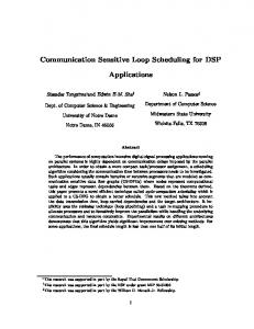
Figure 1: (a) 2-D Mesh (b) a simple CSDFG (c) retimed graph do not consider the parallelism and pipelining across iterations. For scheduling cyclic data- ow graphs, most of the techniques developed for parallel compilers do not consider the communication cost. For example, the technique of software pipelining is used to nd a repeating pattern as a static schedule [1, 8]. Likewise, the polynomial time rate-optimal scheduling without resource constraint for cyclic data- ow graphs proposed by Chao and Sha also does not consider the communication cost [3]. For scheduling tasks on parallel systems, Shukla and Little proposed an algorithm for scheduling task data- ow graphs not considering the imposed communication cost [12]. Munshi and Simons proposed a polynomial time scheduling algorithm for cyclic DFGs without considering communication costs with respect to the processor architecture [10]. Hoang and Rabaey presented a scheduling algorithm which addresses the inter processor communication delays yet the output schedule may be an infeasible schedule if there are smaller number of available processors than its requirement [4]. Chao, LaPaugh and Sha introduced an ecient methodology called the rotation scheduling [2]. This technique optimizes the schedule length by using loop pipelining, but does not consider the communication between processors. A modi ed rotation scheduling strategy dealing with the communication cost was previously proposed for unit-time data ow graphs and completely connected architectures [13]. In this paper, we propose a new and improved scheduling algorithm called cyclo-compaction scheduling which optimizes the schedule length of general-time DFGs with loop carried dependency considering a target architecture and the communication delays between processors. This method focuses on loop pipelining while considering the processor availability and the communication overhead regarding to each particular architecture. The results obtained through the use of this technique are directly applicable to tightly coupled parallel systems, as well as high level synthesis of multi-chip systems. The cyclo-compaction scheduling algorithm schedules nodes in a DFG without violating dependencies and communication constraints. The communication cost is measured by the number of time units required for transmission between processors and the distance between one processor element (sender) and a target processor (receiver). A simple example is shown in Figure 1: a general-time cyclic DFG shown in Figure 1(b) comprising of six tasks (nodes) needs to be scheduled in a 2-D Mesh architecture. The target system is shown in Figure 1(a) with four processor elements (PEs). The computation time of nodes A, C, D, F are assumed to be 1 time unit, nodes B and E are 2 time units. A modi ed list scheduling process gets the initial schedule shown in 2

cs 1 2 3 4 5 6 7 8 9 10 11 12 13 14

pe1 A B B D E E F A B B D E E F

pe2

pe3

cs

pe4

1 2 3 4 5 6 7 8 9 10 11 12 13

C

C

pe1 A B B D E E F A B B D E E F

pe2

pe3

pe4

A C

C

Figure 2: (a) start-up schedule (b) rst iteration cs 1 2 3 4 5 6

pe1 D E E F

pe2 C B B

pe3

pe4

cs 1 2 3 4 5

A

pe1 D E E F

pe2 B B

pe3

pe4

C

A

Figure 3: (a) start-up schedule (b) rst iteration Figure 2(a). This algorithm schedules the nodes by taking into account communication costs with respect to the architecture. Notice that in a system not considering the communication overhead, node C could be parallel to the rst cycle of node B. However, the communication cost with respect to the 2-D Mesh architecture and the dependency between A and C require node C to be scheduled at control step 3 either under processor 2 (PE2) or 4 (PE4) or at control step 4 under processor 3. The algorithm then selected PE2. This initial schedule is then submitted to the novel technique called cyclo-compaction scheduling algorithm. This algorithm rst reschedules node A from control step 1 while implicitly moving one delay from its incoming edges to all of its outgoing edges (see Figure 1(c)). Node A is then assigned to control step 2 (or control step 1 after renumbering the table, Fig. 3(a)) under PE2. After the third iteration, the schedule length is 2 control steps shorter than the initial schedule (see Figure 3(b)). Figure 2 and 3 depict the transformation of the initial schedule table from seven control steps down to ve. Figure 4 shows the nal DFG. The algorithm guarantees that the schedule length at every step is the same length or shorter than the previous one. The remaining of this paper is organized as follows: basic concepts and speci cations of target architectures are presented in section 2. In section 3, mathematical models and basic functions are de ned for the initial scheduling process. Section 4 deals with the optimization of the initial schedule by the technique called cyclo-compaction scheduling . Section 5 provides examples of application to dierent architectures. Finally, a conclusion summarizes the concepts presented in this paper. 3

1

A

3

1

1

B

C

1

1

2

D

E

2

1

1

F

Figure 4: retimed graph after the third iteration

2 Preliminaries This section introduces the de nition of communication sensitive data ow graph , modeled the scheduling problem, and other basic terminologies used in this paper. A communication sensitive data ow graph (CSDFG) G = (V ; E ; d; t; c) is a node-weighted and edgeweighted direted graph, where V is the set of nodes, E  V  V is the set of dependence edges, d is delay between two nodes, t is a function from V to the positive integers representing the computation time of each node, and c is a function from E to the positive integers representing the data volume transfering between two nodes when they are assigned to dierent processors. The notation u ?e! v conveys that e is an edge from node u to node v. The notation upi ?(m!) vpj conveys that there exists a transfering data volume cost m whenever u, executed by processor pi , and v is executed by processor pj . Figure 1(b) depicts an example of CSDFG, where V

A; B; C; D; E; Fg and E = fe1 : (A; B); e2 : (A; C); e3 : (A; E); e4 : (B; D); e5 : (B; E); e6 : (C; E); e7 : (D; A); e8 : (D; F); e9 : (E; F); e10(F; E)g. The delay functions are d(e1) = d(e2) = d(e3) = d(e4) = d(e5) = d(e6) = d(e8) = d(e9) = 0, d(e7) = 3 and d(e10) = 1, the execution time are t(A) = t(C) = t(D) = t(F) = 1 and t(B) = t(E) = 2, and the communication cost for assignment to dierent processors is c(e1) = c(e2) = c(e3) = c(e4) = c(e6) = c(e9) = 1, c(e5) = c(e8) = 2 and c(e7) = 3. An iteration is the execution of each node in V exactly once. Iterations are identi ed by an index i starting from 0. Inter-iteration dependencies are represented by the weighted edges. An iteration is = f

associated with a static schedule. A static schedule must obey the precedence relations de ned by the DFG. For any iteration j, an edge e from u to v with delay d(e) conveys that the computation of node v at iteration j depends on the execution of node u at iteration j - d(e). An edge with no delay represents a data dependency within the same iteration. A legal DFG must have strictly positive delay cycles, i.e., the summation of the delay functions along any cycle cannot be less than or equal to zero.

The clock cycle is the synchronization time interval in the multiprocessor system. A clock cycle is equivalent to one control step in the static schedule. A task that is longer than one clock cycle requires the allocation of resources for multiple control steps. A processing element that has a pipeline design can execute a new task before the completion of the previous one. The retiming technique is a commonly used tool for optimizing synchronous systems [9]. A retiming r is a function from V to integers. The value of this function is the number of delays taken from all incoming 4

(a)

(b)

(d)

(c)

(e)

Figure 5: (a) linear array (b) ring (c) completely connected (d) 2-D Mesh (e) 4-cube edges of node v and moved to each of its outgoing edges and vice versa. An illegal retiming function occurs when one of the retimed edge delays becomes negative. This situation implies a reference to a non-available data from the future iteration. An example of retiming is shown in Figure 1(b) and 1(c). One delay is drawn from the incoming edge of node A and pushed to all of its outgoing edges, see Figure 1(c). Delays are represented as bar lines over the graph edges. A prologue is the set of instructions that must be executed to provide the necessary data for the iterative process after it has been successfully retimed. In our example, the instruction A becomes the prologue. An epilogue is the other extreme, where a complementary set of instructions will need to be executed to complete the process. We may assume that the time required to run the prologue and epilogue are negligible, when compared to the total computation time of the problem. In the rst implementation, the underlying communication cost was assumed to be distributed uniformly via the regular pattern of connection, completely connected [13, 5]. The generalization of architecture are presented below where the communication patterns are predictable. In this paper, we use store and forward technique to hilight the communication cost inherit in any architecture. A Linear Array is the simplest topology and it is one-dimensional connected. N nodes are connected by N - 1 links forming a line , see Figure 5(a). The degree of each node is two except the terminal nodes in the line which have a degree one. When N becomes very large, this connection imposes a communication problem when transfering data between remote nodes. A linear array is proper to implement if the size of N is small. A Ring is obtained by connecting the two terminal nodes of a linear array network as in Figure 5(b). Channels of a ring can either be directed (unidirectional) or undirected (bidirectional). The degree of each 5

node is always two in this symetric topology. On the Completely Connected topology, there are edges connecting each node to every other node, see Figure 5(c). Therefore, every node belonging to this architecture can be reached by any other node through one link. The 2-D Mesh architecture is very popular and implemented in many supercomputers. Interior nodes have degree 4 and the boundary and corner nodes have degree 3 and 2 respectively, see Figure 5(d). A more complex architecture is n-cube shown in Figure 5(e). The number of nodes in an n-cube is N = 2n .

3 Start-Up Scheduling In this section, we modify a traditional list-based scheduling algorithm to be able to deal with both data dependencies and communication delays with respect to a target architecture. Such constraints are parameters in the functions described in this section. Some mathematical models which are required in the algorithm are also presented. We begin by introducing two basic functions which provide information on the execution time of a scheduled node. Since the CSDFG represents a general-time type of data ow graph, the begining and the end of the execution of each node may be associated with dierent control steps respectively designated by the functions CB and CE. We de ne these functions as following:

De nition 3.1 Given a CSDFG G = (V ; E ; d; t; c) and a node u 2 V , the function CB(u), from V to the positive integers, indicates the control step to which u is assigned by the scheduling process, relative to the starting control step of the current iteration. De nition 3.2 Given a CSDFG G = (V ; E ; d; t; c) and a node u 2 V , the function CE(u), from V to the positive integers, indicates the control step at which u nishes its execution, relative to the starting control step of the current iteration, i.e., CE(u) = CB(u) + t(u) - 1. In the example shown in Figure 2(a), CB(B) is 2 and CE(B) is 3. Since the architecture is the other factor needed to take into account, it is necessary to provide a function that returns the assigned processor number for a speci c task. We de ne such a function namely PE as following:

De nition 3.3 Given a CSDFG G = (V ; E ; d; t; c), the function PE(u), from V to the set of processors, de nes the processor assigned to execute the task represented by node u. If no previous assignment exists, the value of PE(u) is unde ned. On the example, PE(B) = 1. In order to obtain an initial schedule considering the communication overhead, a list-based scheduling technique is modi ed. Since the traditional list-based scheduling algorithm does not cover the underlying processor communication constraints, the priority function for this environment needs to be tailored. The following de nitions introduce the functions used to determine the scheduling priority. 6

De nition 3.4 The mobility of a node v, MB(v), is de ned as the dierence between the current control step and the as-late-as-possible control step, a control step in which a node is able to be scheduled as late as possible, that node v can be scheduled without increasing the schedule length (critical path). In order to make the underlying communication cost play a signi cant role, we assume that the communication cost is proportional to the transmitted data volume and the number of links in which transmitted data traverse through. Also the communication channels are multiple so that there is no congestion in transmiting data. The following is the de nition for the communication overhead associated with an architecture.

De nition 3.5 For a given dependency u ?(m!) v in a CSDFG G = (V ; E ; d; t; c), the communication function, M(pi (u); pj (v)), is de ned as the product of the number of links that must be traversed by somedata transmitted from processor pi to processor pj and the transfering data volume cost (m), i.e., in Figure 1(b), if node B was scheduled under PE1 and node E was scheduled under PE3, the communication function would yield 2  3 = 6. From aforementioned observation, it is clear that the topology of the architecture plays an important role in the computation of such functions. For instance, in a linear array of N processors, in order to route from one terminal node to the other end node, the data needs to traverse through N - 1 links. Consequently, we can express the priority function for the initial scheduling algorithm which is modi ed in order that the function perserves both mobility and communication factors. Note that the communication cost in this function is not obtained from the communication function M but m since there is no such an information telling which processor a node is assigned to at this stage. Below we formulate the relationship of all factors as components of the priority function PF.

De nition 3.6 Given a CSDFG G = (V ; E ; d; t; c), a node v 2 V , a set of nodes ui 2 V where ui represents each of the predecessors of v, a processor pj where v can be scheduled, and the data volume m, the priority function PF(v) is de ned as following: PF(v) = maxi;jfm - (cscur - (CE(ui ) + 1)) - MB(v)g where cscur is the current control step being scheduled. The PF function considers all relevant factors that may aect the nal schedule. The cscur - (CE(ui ) + 1) factor implies the number of control steps between the predecessors of ui and the current control step, i.e., how long task v has been delayed after its predecessors have been executed. The the data volume cost m is reduced its eect proportionally to the deferred time. The value of MB(v) function reduces the priority proportionally to how long node v can be delayed without aecting the total execution time. A node with higher mobility (ability of being scheduled later) implies a lower PF. The higher returned value from PF regards as the higher priority of the node to be scheduled.

3.1 Algorithm At this point, we now present the start-up scheduling algorithm based on PF. The input of this algorithm is the CSDFG describing the problem, with no feedback edges. Figure 6(a) shows the input graph with 7

3

A 1

1 1

B

cs 1 2 3 4 5 6 7

C

1

1

2

D

E

2

1

1

F

pe1 A B B D E E F

pe2

pe3

pe4

C

(a)

Figure 6: (a) input graph for start-up scheduling (b) initial schedule respect to our example. This algorithm computes an initial schedule considering communication costs and the target architecture. All nodes which are ready to execute are inserted into a ready list and rearranged according to the priority given from PF function. The algorithm for this initial schedule is shown below.

Algorithm Start-up-Scheduling(G ) Input : CSDFG G = (V ; E ; d; t; c) no feedback edges. Output : A schedule for G . begin cs

0; list ; while V 6=  or list 6=  do dlist  if there exists u 2 V ! no Pred(u) or all Pred(u) have been scheduled. then InsertList(u; list) Arrange(list); while list =6  and Processors-Available do node Extract(list); cm minj fmaxifCE(Predi (node) + M(PE(Predi(node)); pj gg; if cm < cs then Schedule(node; cs; pj ); else dlist dlist [ fnodeg; list list - fnodeg;

endwhile list

end

endwhile

dlist [ list; cs++ ;

On the above algorithm, the PF function is applied inside the routine Arrange. Therefore, the ready node that has the highest priority is scheduled rst. The algorithm attempts to schedule nodes from the list , one by one, according to the priority. It also checks the validity of scheduling the node to an available control step under an available processor by calculating the minimum possible scheduling control step for that speci c position. In the pseudo code above, the algorithm computes the possible control step for the 8

tentative scheduling node by adding the last control step that the parent of the node resided with the communication overhead with respect to a speci c architecture (M). Since it is possible that the node can have multiple number of predecessors, the max function are useful to choose the largest cost among parents. Unlike the cost from multiple predecessors, the min function is applied to determine which processor the node should be scheduled to. The node that cannot be scheduled in the algorithm iteration will be postponed to the next iteration. Finally, the algorithm stops when all nodes have been scheduled. For instance, in the example of Figure 6(a), the algorithm considers the input graph as an acyclic CSDFG. Node A is assigned to the rst available position which is control step 1 under PE1, since node A is the only root of the graph. Thereafter node B and C are ready to be inserted into the list . Both node B and C have equal oportunity to be scheduled. Node B is selected to be scheduled rst at control step 2 under PE1. Nevertheless, because of the communication cost from node A to C, node C cannot be scheduled at the same time as node B; therefore node C is deferred to the next iteration. After node B has been scheduled, node D, the successor of node B becomes ready and it is inserted into the ready list. However the control step 2 is no longer valid for any node inside the list. The algorithm carries out this problem by looking for the next available control step. The algorithm stops when all nodes from the CSDFG have been scheduled. Since the distance between source and destination in 2-D Mesh architecture is not regular, assigning a node to dierent processors causes dierent results. In Figure 6(b), if node C had been spawned under processor PE3, it would need to be scheduled at least at control step 4. Therefore, the algorithm selected to assign node C to control step 3 under PE2. The initial schedule is consequently issued to the cyclo-compaction phase introduced in the next section.

4 Cyclo-Compaction Scheduling This section introduces our optimization algorithm called cyclo-compaction scheduling algorithm. The initial schedule from the previous section will be compacted by this systematical algorithm. The algorithm determines the underlying architecture as part of the rescheduling process. The optimizing system consists of two phases: a remapping phase following a rotation phase which implicitly applies the retiming operation [3]. The cyclo-compaction scheduling deallocates nodes from the rst row of the schedule table and partially maps these nodes to new positions. The rotation phase infers to the movement of delays in the graph. Such a delay movement yields the better pipelining capability of the graph known as retiming. The remapping is essentially partially scheduling process. The follows are the de nition for the rotation phase which extracts nodes from the schdule table while moving delays associated with the nodes in the input graph systematically.

De nition 4.1 Given a CSDFG G = (V ; E ;d; t; c) and J a subset of V , the rotation of set J draws one delay from every incoming edge and pushes it to every outgoing edge of J . The CSDFG is transformed into a new CSDFG, GJ , in a schedule table of length L. This is equivalent to moving the row number 1 to the position L + 1. 9

The rotation holds every property of the retiming operation. Therefore, all of incoming edges of the rescheduled node must have delays greater than zero; otherwise the rotation is regarded as an illegal operation. Note that the rotation operation here is scheduling computing environment in which we are able to consider an intermediate result as an output format. Hence it facilitates the means of solving this problem. The following lemma shows that the rotation per se does not change the schedule length.

Lemma 4.1 Given a CSDFG G , scheduled to be executed according to a schedule table H with length equal to L control steps, the rotation operation retimes G creating a new CSDFG Gr which has the same schedule length L. Proof:

2

Immediate from the de nition of rotation.

As an example, Figure 2(a) and (b) represents the rotation phase of node A, by moving node A from cs1 down to cs8. The remapping operation reschedules it back to cs2 which will be cs1 of the next iteration after renumbering the control steps. There are two approaches of dealing with the remapping, the remapping with relaxation and without relaxation. The former is to allow the schedule length growing larger than the initial one in the intermediate state. The latter is to guarantee that the schedule length will not be longer than the previous one. Both of these methodologies, in fact, produce the nally shorter schedule length by saving the shortest one in every of intermediate step. The basic notion of two remappings are the same. The following de nition represents the concepts of two remapping operations.

De nition 4.2 Given a CSDFG G = (V ; E ; d; t; c), J a subset of V and a current schedule length Li , the remapping without relaxation operation is de ned as assigning nodes in J to the schedule table yielding the shorter or at least the same schedule length Li . Unlike without relaxation, the remapping with relaxation allows to have a longer schedule length Ln > Li . Intuitively, when nodes get re-scheduled with changing delay assignments (retiming) the dependencies within an iteration and between an iteration tend to be modi ed accordingly. The underlying communication cost may imposes an extra length to the new schedule table. Hence, without the relaxation mathod, if the nodes from J are not able to be scheduled to a table in such a way that the schedule length L will be shorter than the former one, the relaxation method will abandon itself. This results at least same schedule length as before according to the lemma 4.1. In other words, the remapping phase does not occur in this case. On the other hand, the remapping with relaxation, is always taken place even if the schedule length becomes longer. Since the communication overheads cause diculties of parallelizing data dependent nodes, every rescheduled node needs to conjecture the position in the schedule table according to the dependencies as well as the communication overheads. The delays of an edge u ?! v imply a dependency between an iteration and if there are no delay, it implies to a direct dependency in the same iteration. For example, in Figure 1(b), the edge D ?! A has 2 delays which means that node A receives the data from a previous execution of node D after two itrations. The edge A ?! B in Figure 1(b) has no delay between them; therefore, both of 10

them must be executed in the same iteration. We formulate the strategy to guess the above constraints as an anticipation function AN described below:

De nition 4.3 Given a CSDFG G = (V ; E ; d; t; c), and k a number of delays in the edge u ?e! v 2 G , the anticipation function of u, AN(u), results in the rst possible control step under a speci c processor such that if node u is assigned to that position, the dependencies and communication constraints between the current iteration and the kth iteration will be held while the resulting schedule length is decreased by one control step. The following lemma represents constraints as the following lemma. i Lemma 4.2 Given a CSDFG G = (V ; E ; d; t; c), a node v 2 V , edges ui ?e! v 2 G , delays of edges after one rotation dr (ei ) > 0, and the schedule length L of the current iteration, after one rotation the rst valid control step for assigning v under a speci c processor pj , in such a way that CB(v) to be inside a schedule length l - 1 with all of the constraints preserved is given by

AN(v) = M(PE(ui); pj ) - (dr (ei )(L - 1) - CE(ui )) + 1 Let L be the schedule length for one iteration. We know that the dierence
between the last control step CE(ui ) and the target schedule length is (L - 1) - CE(u). The minimum number of control steps which satis es the communication requirement with respect to a speci c architecture whenever node u and v are assigned to dierent processors is the value returned from M(PE(u); pj). Therefore, the rst possible control step for v with respect to each u predecessor of v, AN(v) must satisfy Proof:

M(PE(u); pj) =
+ (dr (e) - 1)(L - 1) + AN(v) where (dr (e) - 1)(L - 1) represent the intermediate iterations. Therefore,

AN(v) = M(PE(ui); pj ) - (d(ei )(L - 1) - CE(ui )) + 1 2 The anticipation function computes the expected control step that complies with a schedule length shorter by one. Both of the remapping approaches attempt to partially schedule nodes from J according to the minimum value returned from the anticipation function. Nonetheless, if the target processor is not available at that returned value, the remapping operations will search for the next-minimum-available processor which can be the next minimum returned value from others processors or the next control step under the same resource. For example, in Figure 3(a), node C is rotated and ready to be rescheduled. The remapping phase computes the possible AN(C) for every processor. The AN(C)PE1 = 1 - ((6 - 1) - 6) + 1 = 3, AN(C)PE2 = 0 - ((6 - 1) - 6) + 1 = 0, AN(C)PE3 = 1 - ((6 - 1) - 6) + 1 = 3 and AN(C)PE4 = 2 - ((6 - 1) - 6) + 1 = 4. The minimum returned value of this example would be zero under the same processor as node C's predecessor (PE2); however, the rst available control step of this resource is 4 which is larger than AN(C)PE3 = 3. Consequently, node C is rescheduled to cs3 under PE3. The partial result of this remapping method after the third iteration is shown in Figure 3(b). Nevertheless, for every iteration of the cyclo-compaction algorithm , the deallocation of the rst row from the schedule table may destroy the dependencies between two iterations due to the rotation phase. 11

Therefore, the function called projected schedule length for general-time CSDFGs, PSLG , is applied to compute the required minimum schedule length for each iteration of the cyclo-compaction. Whenever the PSLG value is greater than the remapping-phase schedule length, at most one empty control step is added to the end of the schedule table. In other words, the algorithm will assign empty control step to compensate the communication requirements. It becomes clearer that by the end of the cyclo-compaction iteration, if the remapping without relaxation method is applied and the PSLG returns the longer schedule length, the nodes will not be rescheduled resulting the same length as the previous iteration. On the contrary, the remapping with relaxation technique would permit to have that PSLG length. The PSLG function then is de ned as following:

De nition 4.4 Given a CSDFG G = (V ; E ; d; t; c) and a node u 2 V , the projected schedule length with respect to u, PSLG (u), from V to the positive integers, is the minimum schedule length required to satisfy the data dependency and communication constraints. We formulated the PSLG (u) as the following lemma:

Lemma 4.3 Given a CSDFG G = (V ; E ; d; t; c), an edge u ?e! v 2 G , PE(u) 6= PE(v), and d(e) = k for k > 0, for any iteration i, a legitimate schedule length for G must be greater than or equal to PSLG (u), where & i+k (v) ' M (PE(u); PE(v)) + CE(u) - CB PSL(u) = k Let l be the schedule length for one iteration. We know that the minimum number of control steps between node u at iteration i and node v at iteration i + k is M(PE(u); PE(v)) due to the communication between PE(u) and PE(v). We also know that between iterations i and i + k there are (k - 1) iterations. Since all iterations have the same length l, we can formulate the distance between CEi (u) and CBi+k (v) by: Proof:

M(PE(u); PE(v))  (k - 1)l + (l - CEi (u)) + (CBi+k (v)) +
where
represents an additional number of control steps to allow the data transmission between p(u) and p(v). Rewriting the equation above, we obtain


 M(PE(u); PE(v)) - (k - 1)l - l + CEi (u) - CBi+k (v) In order to obtain a uniform schedule along the entire process execution, we must uniformly distribute
over all k iterations preceding iteration i + k. This distribution, for a minimum
, results in a minimum   value  =
k , and the new static schedule length to satisfy the constraints with respect to node u becomes PSLG(u) =  + l. Substituting and simplifying, we obtain  i i+k  PSLG(u) = M(PE(u); PE(v)) +kCE (u) - CB (v)

2

From the observation of the remapping without relaxation methodology, the cyclo-compaction algorithm will not produce such a longer schedule length for the next optimizing iteration. Hence, we state this property as the following theorem: 12

Theorem 4.4 Given a CSDFG G = (V ; E ; d; t; c), for every pass of the cyclo-compaction scheduling algorithm via the remapping without relaxation method, the resulting schedule length is always less than or equal to the one computed in the previous iteration. During the rotation phase, the algorithm does not change the size of the schedule length according to the lemma 4.1. Likewise, during the remapping phase, nodes are rescheduled only if they t in length(S)- 1 control steps or according to lemma 4.3 their PSLG value is less than or equal to the previous length. Therefore, the schedule length remains the same. 2

Proof:

At this point, we can summarize the cyclo-compaction scheduling algorithm as follows:

Algorithm Cyclo-Compact(G ; z) Input : CSDFG G = (V ; E ; d; t; c). Output : the schedule S. begin

Compute the latest starting time for every u 2 V ; S Start-Up-Schedule(G ); Q S; for (n = 1 to z) (G ; S) Rotate-Remap(G ; S); if (length(S) < length(Q)) then Q S;

end Return(Q)

end Procedure Rotate-Remap(G ; S) begin J fDeallocated nodes from the schedule Sg; GJ Retime(G ; J ); S Remapping(GJ ; J ; S); Return(GJ ; S) end Procedure Remapping(G ; J ; S) begin Compute AN(u) 8u 2 J and 8 processors Reschedule u 2 J such that CB(u)  AN(u) and CE(u) < length(S) and 8v PSLG(v)  length(S) end

5 Examples on Dierent Arichitectures In this section, we present the examples tested on speci c architectures which are linear array, 2-D Mesh, ring, completely connected and 3-cube as shown in Figure 5. We rst begin with the example depicted 13

A B

C

G

D

H

I

F

J

L

K

N

O

E

Q

M

R

P S

Figure 7: CSDFG example containing 19 general-time nodes in Figure 7. A more complex CSDFG comprising of nineteen general-time nodes to be scheduled to 8 processors. In this example, t(C) = t(F) = t(J) = t(L) = t(P) = 2 and the other nodes have execution time equal to 1 time unit shown in Figure 7. With the remapping with relaxation strategy, the resulting schedule tables are issued in the following sequences: In the completely connected architecture, the cyclo-compaction easily attempts distributing nodes from the original graph to every processor so that the schedule length becomes shorter. The following table illustrates how good the algorithms work on the scheduling table with respect to the linear array architecture. For the linear array architecture, nodes originally get assigned to the rst three processors since they do not cause too much trouble with communication constraints. The following table depicts the start-up schedule table. For the ring architecture, an initial schedule table is quite dierent from the linear array since this type of architecture has the connection of two terminal processors. Nodes will be scheduled around the pe1 which are pe2 and pe8 rst (see Figure 8). Unlike the linear array architecture, nodes are distributed to neighbor processors associated with pe1. The start-up schedule table and the schedule table after the cyclo-compaction phase are presented in the following tables: Table 6 presents the resulting schedule table with respect to the ring architecture. The following tables also show the initial schedules as well as the amended table obtained from the cyclo-compaction algorithm with respect to the other two architectures which are 2-D mesh and 3-cube architectures. 14

cs 1 2 3 4 5 6 7 8 9 10 11 12

Start-up Schedule: Completely Connected pe1 A B H G

M P P

pe2

pe3

pe4

pe5

C C I K N O

D

E

F F J J L L Q

R

pe6

pe7

pe8

S

Table 1: the initial schedule table of completely connected

cs 1 2 3 4 5

pe1 E S G A

Completely Connected

pe2 B N L L Q

pe3 M R O

pe4 D H K

pe5 F F J J

pe6 B B I

pe7

pe8

P P

Table 2: the resulting schedule table with respect to completely connected

cs 1 2 3 4 5 6 7 8 9 10 11 12 13

Start-up Schedule: Linear Array

pe1 A B H D G I K N O P P

pe2 C C F F J J L L Q

pe3

pe 4

pe5

pe6

pe7

pe8

E

M R

S

Table 3: the initial schedule table of linear array

15

cs 1 2 3 4 5 6 7

pe1 D E I J J

pe2 S H K

Linear Array

pe3 B F F R C C

pe4 M G A N P P

pe5

pe6

L L Q

O

pe7

pe8

Table 4: the resulting schedule table with respect to linear array

cs 1 2 3 4 5 6 7 8 9 10 11 12 13 14 15

pe1 A B H G

Start-up Schedule: Ring

pe2

pe3

C C

E

I K N O P P

pe4

pe5

pe6

pe7

F F

M R

pe8 D

J J L L Q

S

Table 5: the initial schedule table of ring

cs 1 2 3 4 5 6 7

pe1 J J M R A E D

pe2 C C

pe3 F F

Ring pe4 I

pe5

L L G

pe6

B H

pe7 Q O S

pe8 K N P P

Table 6: the resulting schedule table with respect to ring

16

cs 1 2 3 4 5 6 7 8 9 10 11 12 13

pe1 A B H G I K N O P P

Start-up Schedule: 2-D Mesh pe2

pe3

C C

E

pe4

pe5

pe6

pe7

pe8

D F F J J L L Q

M R S

Table 7: the initial schedule table of 2-D Mesh

cs 1 2 3 4 5 6

pe1 D Q J J E

pe2 F F A S K

2-D Mesh

pe3 M B H G

pe4 L L

pe5 C C I

pe6 N P P

pe7

pe8

R

Table 8: the resulting schedule table with respect to 2-D Mesh

cs 1 2 3 4 5 6 7 8 9 10 11 12 13

pe1 a B H G I K N O P P

Start-up Schedule: 3-cube pe2

pe3

C C

D F F J J L L Q

pe4

pe5

pe6

pe7

pe8

E

M R

S

Table 9: the initial schedule table of 3-cube 17

cs 1 2 3 4 5 6

pe1 N P P D Q S

pe2 H G J J F F

pe3 M A R B

3-cube pe4

pe5

pe6

L L E

O

K

pe7

pe8

C C I

Table 10: the resulting schedule table with respect to 3-cube Applications

relax

Elliptic Filter Latice Filter Elliptic Filter Latice Filter

w/o with

Testing on applications

com init after 126 126 105 100 105 35 126 57

init 126 105 105 126

lin after 126 100 49 85

init 126 99 99 122

rin after 126 93 65 99

init 126 99 99 122

2-d after 126 93 65 95

init 126 105 105 126

hyp after 126 103 37 71

Table 11: Applying Cyclo-compaction on dierent architectures The examples above have demonstrated the fast convergence characteristic of the algorithm and its eciency. It also corroborates the notion that the performance of the system would be better in the completely connected architecture than the other architectures because of the uniformity of communication cost among processors. The table 11 persents the other two examples, the 5th eliptic and lattice lter with a slow down factor of 3 comparing two remapping strategies with respect to the 5 architectures, completely connected, linear array, ring, 2-D Mesh, and 3-cube . The \init" column represents the start-up schedule length for each application and the \after" column shows the resulting schedule length. From the information in table 11, the completely connected architecture seems to give out the shortest schedule table of all. The remapping scheme with relaxation yields the better result eventhough the intermediate scheduling process may give the longer schedule table according to the PSLG.

6 Conclusion Previous scheduling mechanisms are restricted to non-cyclic data ow graphs or do not consider communication overhead that exists when two tasks, i.e., nodes in the data ow graphs are spawned to dierent processors. This paper presented a new algorithm called cyclo-compaction scheduling to schedule cyclic data ow graphs with loop carried dependencies, taking into account communication costs for a speci c architecture. Our algorithm compacts a given initial schedule iteratively by rotation and remapping. The retiming (or loop pipelining) is implied in each of our rotation steps, and remapping is performed to map rotated nodes to the best processor while communcation overhead and dependency legality are considered. According to our experiments, this algorithm gives a much shorter legal schedule for all kinds of parallel architectures. 18

1

2

3

7 8

7

8

(a)

6

1

5

2

5

6

7

1

2

3

(b)

8

4 3 (c)

7

8

4 (d)

4

3

6

5 1

(e)

2

Figure 8: the experiment architecture (a) linear array (b) ring (c) completely connected (d) 2-D Mesh (e) 3-cube

References [1] A. Aiken and A. Nicolau. Optimal loop parallelization. In Proc. of the ACM SIGPLAN Conf. on Programming Languages Design and Implementation, pages 308{317, June 1988. [2] L. Chao, A. LaPaugh, and E. Sha. Rotation scheduling: A loop pipelining algorithm. In Proc. of ACM/IEEE Design Automation Conference, pages 566{572, Dallas, TX, June 1993. [3] L. Chao and E. Sha. Uni ed static scheduling on various models. In 1993 Int. Conference on Parallel Processing, pages 231{235, St. Charles, IL, August 1993. [4] P. D. Hoang and J. M. Rabaey. Scheduling of dsp programs onto multiprocessors for maximum throughput. IEEE Transactions on Signal Processing, 41(6), June 1993. [5] K. Hwang. Advanced Computer Architecture: Parallelism, Scalability, Programmability. McGrawHill Series in Computer Science, New York, NY, 1993. [6] R. A. Kamin, G. B. Adams, and P. K. Dubey. Dynamic list-scheduling with nite resources. In Int. Conference on Computer Design, pages 140{144, October 1994. [7] A. A. Khan, C. L. McCreary, and M. S. Jones. A comparison of multiprocessor scheduling heuristics. In 1994 Int. Conference on Parallel Processing, volume II, pages 243{250, 1994. [8] M. Lam. Software pipelining. In Proc. of the ACM SIGPLAN Conference on Progaming Language Design, pages 318{328, 1988. [9] C. E. Leiserson and J. B. Saxe. Retiming synchronous circuitry. Algorithmica, pages 5{35, June 1991. [10] A. A. Munshi and B. Simons. Scheduling sequential. SIAM Journal of Computing, 19:728{741, August 1990. 19

[11] B. Shirazi, K. Kavi, A. R. Hurson, and P. Biswas. Parsa: A parallel program scheduling and assessment environment. In 1993 Int. Conference on Parallel Processing, January 1993. [12] S. Shukla and B. Little. A compile-time technique for controlling real-time execution of task-level data- ow graphs. In 1992 Int. Conference on Parallel Processing, volume II, 1992. [13] S. Tongsima, N. L. Passos, and E. Sha. Communication sensitive rotation scheduling. In Int. Conference on Computer Design, October 1994.

20