The Cryosphere
Open Access
The Cryosphere, 7, 1887–1900, 2013 www.the-cryosphere.net/7/1887/2013/ doi:10.5194/tc-7-1887-2013 © Author(s) 2013. CC Attribution 3.0 License.
Arctic Ocean sea ice snow depth evaluation and bias sensitivity in CCSM B. A. Blazey1,2 , M. M. Holland3 , and E. C. Hunke4 1 Center
for Marine Environmental Sciences (MARUM), Universität Bremen, Bremen, Germany of Atmospheric and Oceanic Sciences, University of Colorado, Boulder, Colorado, USA 3 National Center for Atmospheric Research, Boulder, Colorado, USA 4 Los Alamos National Laboratory, Los Alamos, New Mexico 2 Department
Correspondence to: B. A. Blazey (
[email protected]) Received: 1 March 2013 – Published in The Cryosphere Discuss.: 9 April 2013 Revised: 21 October 2013 – Accepted: 26 October 2013 – Published: 13 December 2013
Abstract. Sea ice cover in the Arctic Ocean is a continued focus of attention. This study investigates the impact of the snow overlying the sea ice in the Arctic Ocean. The impact of snow depth biases in the Community Climate System Model (CCSM) is shown to impact not only the sea ice, but also the overall Arctic climate. Following the identification of seasonal biases produced in CCSM simulations, the thermodynamic transfer through the snow–ice column is perturbed to determine model sensitivity to these biases. This study concludes that perturbations on the order of the observed biases result in modification of the annual mean conductive flux through the snow–ice column of 0.5 W m2 relative to an unmodified simulation. The results suggest that the ice has a complex response to snow characteristics, with ice of different thicknesses producing distinct reactions. Our results indicate the importance of an accurate simulation of snow on the Arctic sea ice. Consequently, future work investigating the impact of current precipitation biases and missing snow processes, such as blowing snow, densification, and seasonal changes, is warranted.
1
Introduction
The decline of Arctic Sea ice extent over recent decades is well documented (Parkinson et al., 1999; Meier et al., 2007). This decline continues unabated, with the period 2007–2013 setting records for six of the seven lowest summer ice extents since the beginning of the satellite record (NSIDC, 2013). Last summer, 2012, set the record for the lowest summer ice
area (NSIDC, 2012). The high sensitivity to climate change in the Arctic (Holland et al., 2006a, b) combined with anticipated feedback mechanisms, such as the ice albedo feedback (Curry et al., 1995), warrants a continued focus on realistically simulating the Arctic system in large-scale climate models. In addition, while the model representation of the transition from a perennial to a seasonal ice pack is improving, this shift continues to progress more quickly than simulated by many general circulation models (Stroeve et al., 2007, 2012). Major shifts in the character and age of the ice are indicative of a persistent shift in the state of the Arctic ice cover (Maslanik et al., 2007, 2011). These changes include a shift to a younger, thinner, and more seasonally variable ice pack. As the ice in the Arctic Ocean becomes more similar to the ice in the Southern Ocean, it may be that features such as snow depth will increase in importance to the Arctic sea ice (Fichefet and Maqueda, 1999), and in turn to the regional climate. In addition to changes in the ice itself, the overlying snowpack is projected to decline in the Arctic in several GCMs (Hezel et al., 2012; Vavrus et al., 2012). These changes are projected to significantly impact the thermodynamics of the sea ice (Blazey, 2012). This highlights the need to examine thermodynamic processes controlling the evolution and state of the Arctic ice pack. The thermal conductivity of snow is nearly an order of magnitude less than the thermal conductivity of the ice it covers, and as such snow depth is an important component of the thermal transfer through the ice column despite its relatively tenuous nature. In previous sensitivity studies using models, the net effect of snow depth on the ice pack varies.
Published by Copernicus Publications on behalf of the European Geosciences Union.
1888
B. A. Blazey et al.: Arctic Ocean sea ice snow depth evaluation
One of the earlier model sensitivity studies of sea ice found that snow on sea ice has two primary competing effects on the ice mass budget (Maykut and Untersteiner, 1971). During the ice growth season, the presence of snow insulates the sea ice, reducing the transfer of heat from the ice–ocean interface. This in turn reduces ice growth. However, in the transition to the surface ice melt season, the presence of snow can delay surface ice melt and lead to a reduction in the seasonal ice mass loss. The high albedo of snow relative to sea ice also plays an important role in the surface heat budgets and the onset of ice melt. While Maykut and Untersteiner (1971) identified the major processes by which snow modulates the ice thermodynamics and mass balance, they found that in the idealized model these effects were balanced for snow depths ranging from 0 to 70 cm. However, this finding did not hold with subsequent studies. Later studies, undertaken both in situ and using various modeling environments, have found a variety of responses to snow depth. For example, Brown and Cote (1992) found ice thermodynamics, including ice growth, to be highly sensitive to snow cover, while Holland et al. (1993) found snow to be of secondary importance to ice characteristics. Fichefet and Maqueda (1999) found the ice cover in the Southern Ocean to be “remarkably sensitive to the accumulation rate of snow”. Massom et al. (2001) observed the highly complex and variable role of snow on Antarctic sea ice. The authors concluded that a proper treatment of snow on sea ice is important to climate modeling. Cheng et al. (2008) found snow depth to be an important element in the sea ice system within a modeling environment. While more recent studies have explored the introduction of additional thermodynamic complexity to the treatment of snow (Lecomte et al., 2011; Cheng et al., 2008), these studies have focused on one-dimensional modeling and evaluation. The role of snow cover in modulating ice growth has been verified in the field, where the heterogeneity of snow distribution has been observed to produce corresponding heterogeneous growth in underlying lake ice (Sturm and Liston, 2003). More specifically, focused snow thermal conductivity sensitivity studies have found a 10–20 % change in ice thickness when snow thermal conductivity is halved from the typical ∼ 0.3 W m−1 K−1 to the measured value of 0.15 W m−1 K−1 (Sturm et al., 2002; Wu et al., 1999; Fichefet et al., 2000). Considering the range of findings in previous investigations of the net role of snow depth to the sea ice mass thermodynamics, we are motivated to investigate this aspect of the Arctic climate system in one of the major current GCMs. As such, this study evaluates the snow depth and density over sea ice as simulated in Community Climate System Model (CCSM) fully coupled runs using in situ measurements of snow depth. Sensitivity runs are then performed to determine the influence of snow depth and density biases on both the ice state and the Arctic climate. Additional evaluations of snow characteristics and simulations of the stand-alone ice model The Cryosphere, 7, 1887–1900, 2013
the Community Sea Ice Code (CICE) were also performed and are reported in Blazey (2012). These simulations found consistent ice sensitivity to decreases in snow depth and a mean state-dependent response to increases in snow depth. Due to the coupled nature of these simulations, we expect initial perturbations to the ice caused by changes to the snow characteristics to result in feedbacks with other components of the Arctic climate system. Section 2 describes the GCM utilized: CCSM4 and its component ice model, CICE. Section 3 describes the in situ measurements and evaluation method. Section 4 discusses evaluation of CCSM, including possible causes of snow depth biases identified therein. Section 5 details the design and results of the CCSM bias sensitivity experiment. Section 6 begins with a discussion of the implications of our results with regards to the CICE and the CCSM results as a whole. We conclude with a discussion of future directions for this work. 2
Model: CCSM4
CCSM4, released in Spring 2010, includes coupled component models for the atmosphere, ocean, ice, and land surface and is mass and energy conserving. This study makes use of CCSM in two configurations. For the evaluation portion of this study, the release version of the CCSM4 is used with all components active. The sensitivity portion of this study utilizes a reduced version of CCSM with the fully active ocean replaced by a slab ocean model (SOM). Here we focus on the sea ice component model and improvements to CCSM most important to the Arctic Ocean. A more comprehensive discussion of the improvements in CCSM4 is available in Gent et al. (2011). The sea ice component model used in CCSM4 is the Los Alamos Sea Ice Model (CICE) version 4 (Hunke and Lipscomb, 2010). CICE is designed to be computationally efficient while including a thermodynamic model, a model of ice dynamics, a transport model that describes advection, ridging parameterization, and a sub-grid-scale ice thickness distribution (Thorndike et al., 1975). CICE includes elastic–viscous– plastic dynamics (Hunke and Dukowiz, 2002) and is energy conserving (Bitz and Lipscomb, 1999). In the default configuration, CICE has a 30 min time step, 4 ice layers and 1 snow layer; however these values can be changed. In the configurations used in this study, the sub-grid-cell ice thickness includes five prescribed thickness categories. Each category includes a discrete thermodynamic treatment including snow calculations. These calculations are uniform across each grid cell at each time step. Ice and snow are transferred between categories by means of a one-dimensional linear remapping (Lipscomb, 2001) and include deformation, dynamical advection, and thermodynamic thickness change as pathways. Spatial advection occurs by means of a two-dimensional linear remapping (Lipscomb and Hunke, 2004).
www.the-cryosphere.net/7/1887/2013/
B. A. Blazey et al.: Arctic Ocean sea ice snow depth evaluation In general, the thermodynamic and dynamic treatment of snow follows the treatment of the ice. However, snow is only transferred between ice thickness categories or grid cells with the ice it overlies. As such, the snow overlying the sea ice can be considered a feature of the ice, rather than an independent process. However, there are a handful of processes where the snow is treated separately. Other than precipitation and melt these include snow-to-ice formation and loss of snow mass during ice deformation. Recent improvements to CICE include a delta-Eddington (DE) multiple scattering treatment of snow and ice, which uses internal snow properties to determine albedo and sets CICE ahead in relation to most GCMs (Briegleb and Light, 2007). In the DE parameterization of CICE, surface albedo is computed using the thickness of snow and ice, in combination with a melt pond layer. Parameters such as snow grain size are also included, and the treatment compares favorability with in situ measurements. However, neither temperature nor snow age is considered. This may potentially lead to biases in the surface albedo, considering the large changes in snow albedo as snow ages and melts (Perovich et al., 2002, 2007). The melt and aging of snow and sea ice lead to large albedo decreases, upward of a factor of 2 in the case of snow alone (Perovich et al., 1998). However, investigating the impact of snow and albedo treatment biases is beyond the scope of this work. For purposes of this study we consider the deltaEddington treatment to be an adequate albedo. CICE now includes a non-zero heat capacity for the snow cover, melt ponds, and aerosol deposition. The effects of this parameterization are reported in Holland et al. (2012). Despite these improvements, the density and thermal conductivity of snow in CICE are fixed. As a result, the treatment of CICE snow is more rudimentary than the treatment of snow in the Community Land Model (CLM) (Lawrence et al., 2011; Olsen et al., 2010). Additionally, CICE does not currently include blowing snow, which has been found to significantly reduce snow depth biases in a focused snow model environment via snow loss to leads (Chung et al., 2011; Déry and Tremblay, 2004). However, the advection of ice cover presents a distinct challenge for snow treatment by CICE in comparison to CLM, and is not included in most model environments. Moreover, the actual snow depths produced in simulations including CICE have not been validated. The atmospheric component model, the Community Atmospheric Model version 4 (CAM4), includes 26 vertical layers with a resolution of 1.25◦ by 0.9◦ . CAM4 uses a LinRood dynamical core (Lin, 2004). For a more detailed description of CAM4, see Neale et al. (2013). In the Arctic, the inclusion of a freeze dry modification serves to reduce the winter low-level clouds in the Arctic (Vavrus and Waliser, 2008). The land model, the Community Land Model version 4 (CLM4), uses the same grid as CAM4, and includes improvements to hydrology. CLM4 makes use of the Snow and Ice Aerosol Radiation model (SNICAR) (Flanner et al., 2007), www.the-cryosphere.net/7/1887/2013/
1889
and includes grain-size-dependent snow aging, aerosol deposition, and vertically resolved snowpack heating. For full documentation, see Lawrence et al. (2011) and Oleson et al. (2010). The Parallel Ocean Program version 2 (POP2) is the ocean component of CCSM4. POP2 uses a 1-degree grid with the North Pole displaced into Greenland. POP2 uses 60 vertical levels, with a surface layer thickness of 10 m, increasing with depth (Smith et al., 2010). Improvements to POP2 include mixing parameterizations allowing improved simulation of North Atlantic dense water transport (Briegleb et al., 2010; Danabasoglu et al., 2010). In order to save computation time, the fully active POP2 is replaced with a SOM in the sensitivity experiments described in Sects. 4 and 5. The SOM serves as a heat reservoir, while calculating a surface ocean temperature for a fixeddepth layer using a surface energy budget calculation and a prescribed ocean heat transport (Bitz et al., 2011). This prescribed transport is obtained from coupled simulations (Bailey et al., 2012). As a result, additional processes such as currents and oceanic transport are omitted. Our simulations use the SOM rather than the full POP2 in large part due to the lower computational costs, a result of both the simplified model and the faster equilibration of the model. Danabsoglu and Gent (2009) found that the results of the SOM and fully coupled simulations were similar under control conditions, with differences under a perturbed climate focused in the Southern Ocean. The model output hereafter referred to as CCSM makes use of a six-member ensemble of fully coupled 20th-century simulations (Gent et al., 2011). Each ensemble member is simulated over the period 1850–2005 and includes anthropogenic effects for this period. The general performance of CCSM4 in this ensemble is available in Gent et al. (2011). More specifically, discussions of the Arctic region performance for this ensemble are available in the CCSM special collection of the Journal of Climate for atmosphere (de Boer et al., 2012) and sea ice/ocean (Jahn et al., 2012) conditions.
3 3.1
Snow depth evaluation In situ data
The primary source of in situ snow measurements is Russian drift stations (Arctic Climatology Project, 2000). These stations were located on multiyear ice, and at least one station was in operation during the period 1954–1991. Snow depth measurements were made in two ways. First, an ideally daily observation occurred at a snow stake adjacent to the ice camp. Second, once to thrice monthly, a 500 m to 1000 m transect “snow line” was made at least 500 m from the camp. Snow depth was measured every 10 m along this transect. In addition to depth, snow density was measured using a cylinder massing technique. Transects were made when The Cryosphere, 7, 1887–1900, 2013
1890
B. A. Blazey et al.: Arctic Ocean sea ice snow depth evaluation
snow depth exceeded 0.05 m and covered at least 50 % of the transect length. Subsequent transects would occur in the same direction but offset several meters. When making use of transect snow measurements, we consider the mean of a transect value (depth or density) to constitute a single measurement. While it would be natural to assume the snow stake measurement could be contaminated by snow alteration due to proximity to the ice camp, Warren et al. (1999) did not find this to be the case. However, Warren et al. (1999) did favor using the transect snow depths when generating a snow climatology. While the in situ measurements are used for the point-by-point model data comparison, this study does make use of the Warren et al. (1999) snow climatology when comparing the geographic distribution of snow depth. Ice mass balance (IMB) buoys managed by the Cold Regions Research and Engineering Laboratory (CRREL) were considered as an additional source of in situ snow depth data (Perovich et al., 2009). However, the buoys’ advection paths along the eastern coast of Greenland were found to cause difficulty matching the buoys to appropriate model grid cells. For a discussion of this issue see Blazey (2012). 3.2
Evaluation method
Due to using an ensemble of fully coupled historical forcing simulations (hindcasts), we do not expect that the model will capture the depth of snow in a given year in the in situ measurements. Instead, we examine the ability of the model to produce both reasonable mean monthly snow depths, and reasonable variation from the mean in comparison to the in situ measurements. As such, we regard the hindcast snow depths and in situ measurements to be independent samples, with each sample being a snow depth in a given month. In the method that follows, we use a selection process to compare ice of similar geographical location, historical period, and characteristics to the in situ measurements. In the model ensemble used, monthly mean model states are saved. As such, in situ measurements discussed in the previous section are matched to a single monthly output file. In this way, the sample size of the snow line measurements and matched model grid cells are equal. In the case of the snow stake measurements, the drift of the station results in 1 to 30 snow stake measurements per matching grid cell. In both cases, we compare the monthly mean snow depth for the period 1954–1993. A given in situ measurement is compared to the model grid cell with the closest center point, with the following selection criteria. The matched CCSM locations are restricted to grid cells above 70◦ N, which eliminates the seas along the margin of the Arctic. Each in situ measurement is matched to two model grid cells. The first is the nearest grid cell, poleward of 70 N, with at least 15 % ice cover, hereafter referred to as the “all_ice” snow thickness, as all ice cover is considered. This definition of ice cover corresponds to commonly used ice extent definitions (ex: Meier et al., 2007). However, 15 % The Cryosphere, 7, 1887–1900, 2013
ice cover does not correspond well with the ice conditions in which the in situ measurements were made since the stations were located in areas of high-concentration, multiyear ice. To better match the thicker multiyear ice conditions of the Russian stations, this matching process is repeated with the selection restricted to the nearest grid cell, north of 70 N, with at least 50 % of the cell covered with ice greater than 1.5 m thickness. We refer to this snow depth as the “thick_ice” depth. A thickness of 1.5 m is used because it is the maximum thickness of the second of five thickness categories. In general, the exact choice of thickness does not affect the snow depth. In the case of monthly snow line measurements, the mean of the transect is taken as the sample, resulting in equal sample sizes for the in situ measurement and model values. In the case of the daily snow stake measurements, the drift of the station itself results in multiple model grid cells corresponding to a given set of monthly measurements. In a representative hindcast, if all_ice matching is used there is a mean of 4.5 in situ measurements per matched model grid location. If the thick_ice matching is used, there are 4.4 in situ measurements per model location. In general, restricting the matching to model locations with thick_ice results in slightly greater distances between the matched in situ and model locations. The distance increases a mean of 17 km to 23 km in the case of the monthly transects, and from 21 km to 25 km in the case of the daily stake measurements. Using these two methods, a reasonable comparison of CCSM-produced monthly mean snow depths for the period 1954–1993 is performed. Following the matching process we have matched data sets of snow depth: transect to all_ice thicknesses, transect to thick_ice, and similarly for snow stake measurements. A paired Student’s t test was performed on each pair by month. Again, we do not expect the samples to be exactly matched due to the model’s inability to simulate a given year. However, by matching time of year, geographical location, and year (mostly for era, not particular year), we produced paired samples. The degrees of freedom vary significantly, from as little as 3 in the summer for the transect to 2000 for the snow stake measurements. With the exception of summer, the DOF for the transect is approximately 50 for each month, and 2000 for the snow stake. 3.3
CCSM snow evaluation results
Unsurprisingly considering the excessive precipitation produced by CAM in the Arctic (de Boer et al., 2012), and lack of blowing snow in CICE, the comparison indicates significant snow depth and density differences between the CCSM ensemble and the in situ measurements. Figure 1 shows the model snow depths in relation to the in situ measurements. At a qualitative level, CCSM4 snow depths are generally too thick relative to the in situ measurements. CCSM snow depths are 20 % in excess of Russian drift station transects on all_ice, and 30 % in excess on thick_ice. www.the-cryosphere.net/7/1887/2013/
B. A. Blazey et al.: Arctic Ocean sea ice snow depth evaluation These excesses are much higher by midsummer, and in August reach 80 % and 105 %, respectively. The average mean annual biases in absolute terms are 4.7 cm and 6.4 cm, while the August values are actually higher, 6.9 cm and 7.7 cm, for all_ice and thick_ice, respectively. The differences between the CCSM snow depths (for both all_ice and thick_ice) of the individual ensemble members in Fig. 1 are not necessarily statistically significant (p < = 0.05) in comparison to the Russian in situ data. When considering individual ensemble members, the most likely months to lack statistically significant differences in snow depths are June, July, and August. This is likely due to a low number of in situ samples for the summer period. However, taken as an ensemble, the differences for the CCSM snow depth differences (both all_ice and thick_ice) are statistically significant for all months except July when validated against the Russian drift station transect data. In addition, the Russian drift station transect data has a lower standard deviation in snow depth than the model, a mean of 30 % of the total snow thickness, in comparison to 54 % and 49 % for the corresponding all_ice and thick_ice CCSM snow thickness. It is unsurprising that the all_ice comparison produces the largest variance, as ice of highly variable thickness is selected. As a result, thin ice that has accumulated little snow is included in this population. The snow stake average standard deviation, 64 %, is larger in part due to each value being a single measurement, rather than a mean of many measurements. The two in situ variances bracket the 51 % and 48 % mean standard deviations for the corresponding CCSM all_ice and thick_ice snow depths, as detailed below. Because the CCSM snow depths are averaged over a grid cell, rather than the point measurements of the snow stake in situ measurements, the lower standard deviations for these snow depths are unsurprising. CCSM snow depth biases are slightly higher in relation to the Russian drift station snow stake measurements. The all_ice snow depth excess is greater than 20 %, and the thick_ice snow depth excess is greater than 50 %. As with the snow line, the modeled snow biases relative to the snow stake measurements are very high in the summer, exceeding 80 % and 195 % in August. The significance of these comparisons is very similar to the transect comparisons: all months except July satistfy our significance test (P < 0.05) Next, the geographical distribution of the thickness bias is examined, as shown in Fig. 2. In general, it appears that the CCSM ensemble produces a snow depth excess of about 20 cm near the Canadian Arctic Archipelago when compared to the Warren et al. (1999) climatology. This excess is most pronounced in the winter and summer (as opposed to the fall freeze-up) when CCSM produces snow greater than 50 cm thick and the in situ snow climatology is ∼ 30 cm thick in this region. However, note that this occurs in the regions of thickest ice, along the Canadian Arctic Archipelago. There is a lack of Russian drift stations used by Warren et al. (1999) in this region, as shown by the symbols in Fig. 2. However, exwww.the-cryosphere.net/7/1887/2013/
1891
trapolation of the snow depths from central Arctic stations indicates thicker snow does accumulate in the vicinity of Greenland and the Canadian Arctic Archipelago. The snow climatology reproduced in the bottom row of Fig. 2 suggests the thickest snow was observed on this side of the Arctic. It seems possible that very deep snow does occur in this region of the Arctic Ocean, but additional station coverage would be required to detect this feature. Regardless, while CCSM is producing too much snow depth overall, the highest biases are in the area where the thickest snow depths are expected. Finally, Fig. 3 documents density bias between the measurements made as part of the Russian snow depth transect and the CICE default snow density of 330 kg m−3 (Hunke and Lipscomb, 2010). Note that no snow density measurements were made in July and August. The most apparent difference results from the omission of snow densification by the invariant snow density in CICE. As a result, the snow density is approximately 30 % too great in the early autumn, but is approximately correct by the onset of melt. This implies that the excess in snow mass, or snow water equivalent, is larger in the fall than the depth comparison would imply. Overall, we find that the CCSM ensemble produces yearround excesses in snow depth, for both of the in situ measurements (stake and transect) used for evaluation of CCSM. Two potential causes of this excessive snow depth come to mind. First, the CAM produces excessive Arctic precipitation (de Boer et al., 2012). Second, CICE does not treat the loss of blowing snow to leads and sublimation, which was found to reduce high biases in modeled snow depth (Chung et al., 2010). The excess is especially pronounced in the summer months. In addition to depth biases, the use of a fixed snow depth parameter results in snow that is too dense in the fall, but is much nearer the in situ measurements by the onset of the spring and summer melt.
4 4.1
Bias sensitivity simulation CCSM bias sensitivity simulation design
The sensitivity portion of this study seeks to determine the effects of snow depth and density biases on ice characteristics and the controlling thermodynamics. Biases in the snow cover will impact the insulating properties of the sea ice, with implications for ice growth and melt. Both are important processes that can lead to biases in the simulated sea ice mass budgets. The general method is intended to assess the effects of snow depth changes of a magnitude equal to the bias we reported in Sect. 3.3 on the Arctic ice cover and climate. Specifically, we modify the thermal conductivity of the snow in CCSM/CICE to account for the observed bias in snow depth. As such, the ice will experience the snow as having the thermal conductivity of a thinner snowpack. Snow conductivity has previously been shown to have an impact on sea ice growth in a model environment (Fichefet et al., 2000). The Cryosphere, 7, 1887–1900, 2013
1892
B. A. Blazey et al.: Arctic Ocean sea ice snow depth evaluation
Fig. 1. Panels (a) and (b): CCSM Arctic Ocean snow depths for the period 1954–1993 validated against Russian drift station measurements. Panel (a) displays the Russian snow line as the in situ data; panel (b) uses the Russian snow stake as the in situ data. Each ensemble member is reported separately. Black squares indicate the in situ values for the period; red diamonds indicate the snow depth overlying the nearest ice of any thickness; blue asterisks indicate the snow depth overlying the nearest ice with greater than 1.49 m thickness. Vertical bars indicate one standard deviation for both in situ and model snow depths.
Fig. 2. Geographical distribution of modeled snow depth and in situ measurements, in cm. As defined by the color bar, red corresponds to low snow depth and blue to high snow depth. From left to right: winter (January, February, March), summer (June, July, August), and freeze-up (October). The top row is the CCSM ensemble snow depth climatology. The second row overlies the position of the Russian drift station locations over a snow depth climatology derived from the in situ measurements taken at these stations (Warren et al., 1999).
While the basic principle has previously been documented, this study extends previous work by investigating the role of feedback processes between the sea ice, atmosphere, and surface ocean. While altering density and snow thickness directly would be the most straightforward method to explore biases in these quantities, such alterations pose difficulties surrounding mass and energy conservation. More specifically, reducing the precipitation mass at the coupling interface between The Cryosphere, 7, 1887–1900, 2013
Fig. 3. Snow density bias: CICE model default less in situ measurements; bars indicate standard deviations (in the in situ measurements.
CAM and CICE would result in the removal of precipitation mass and the thermal energy present in the mass from the model environment. Instead, to assess the implications of the snow biases for sea ice thermodynamics, we manipulate the snow thermal conductivity. This method allows us to investigate the thermodynamic role of snow in the thermal transmittance through the snow–ice column. To better understand this process, it is useful to consider thermal transmittance, Utotal , in Eq. (1), which is the rate at which energy is transferred through a barrier of a given thickness under steady-state conditions. However, note that this is not a part of the CICE model, and is used here only for clarity. Thermal transmittance is useful to consider here because there are two barriers present in the sea ice system, ice and snow. Thermal conductivity, k, is the rate of transfer through a barrier per www.the-cryosphere.net/7/1887/2013/
B. A. Blazey et al.: Arctic Ocean sea ice snow depth evaluation unit thickness, h, and is a characteristic of the material. In Eq. (1) h/k can be considered a thermal resistance, and is cumulative as in Eq. (1). In Eq. (1), Utotal is the total thermal transmittance, here a function of the snow and ice thermal conductivities (ksnow , kice ) and thickness (hsnow , hice ). It is useful to consider Eq. (1), the control situation. Utotal =
1 hice kice
(1)
snow + hksnow
For purposes of this sensitivity study, we wish to adjust the value of ksnow to ksensitivity , a conductivity used to make the snow appear “correct” thermally, as in Eq. (2). Usensitivity =
1 hice kice
hsnow + ksensitivity
(2)
We adjust the conductivity such that the snow thermal transmittance accounts for the bias in model snow depth and density described earlier. Beginning with depth adjustments, we take the product of ksnow and hinsitu / hsnow(eval) , where hinsitu is taken from the in situ measurements, and hsnow(eval) is the CCSM snow depth matched to the in situ measurements. The adjusted snow thermal conductivity reported in Eq. (2). By way of example, if the CCSM snow is too thick, the snow thermal conductivity is effectively reduced to adjust for this, causing the thermodynamics to experience a thinner snow cover. kh
sensitivity
= ksnow
hsnow(eval) hinsitu
(3)
Next, Eq. (2) is adjusted by the addition of a ρinsitu /ρsnow density values for the in situ measurements and default CICE snow densities, effectively adjusting the effective snow depth to account for density biases. The final modified conductivity is reported in Eq. (4). This conductivity is applied in the CCSM conductivity experiment. ksensitivity = ksnow
hsnow(eval) ρinsitu hinsitu ρsnow
(4)
An average of the monthly bias derived from the snow stake bias and snow line bias is used to calculate the biases tested in this section. This is a simpler method than that used by Warren et al. (1999) in the development of their climatology, but will serve to determine whether the biases are relevant to the state of the Arctic ice. In addition, rather than consider the direct effect of snow density on conductivity as determined by Sturm et al. (1997), the bias correction instead compensates for the excessive snow density early in the season by mimicking a thicker snowpack, which would contain the same snow mass per unit area while having a lower density. We consider a linear relationship between excessive snow density and the total thermal resistance presented by the snow cover. This likely results in a lesser effect on snow thermal conductivity than a www.the-cryosphere.net/7/1887/2013/
1893
full treatment of the complex relationship between density and conductivity, but our results still reflect the role of the more complex relationship. However, it is important to note that because this method does not change the snow mass, the thermal diffusivity is not altered. As a result, the perturbation introduced is a lesser effect than a fully bias corrected snow depth would trigger. Figure 4 presents the new conductivities used. While values are calculated monthly, the values are interpolated at each model time step. This avoids discontinuities in the conductivity. Note that the higher conductivities in the CCSM bias experiment compensate for the excess snow depth, and will allow for more thermal transfer through the snow–ice column. In this way, the ice will experience the thermal effect of a thinner snow cover, correcting for the snow depth and density bias. The sensitivity experiments are integrated over a period of 60 yr. As the results indicate, this is sufficient to allow the CCSM and CICE to come to quasi-equilibrated states. Because we use the SOM, there is no ocean to equilibrate, but by leaving CAM and CLM active the Arctic atmosphere and adjacent landmass are allowed to respond to changes in the ice cover. In addition, we are able to assess the impacts of the changes in sea ice on the overall Arctic climate, in particular the overlying atmosphere. 4.2
CCSM bias sensitivity simulation results
We begin with a discussion of the changes to the ice state during the equilibrated period of the simulation, defined as the last 20 yr of a 60 yr simulation. Following the discussion of the equilibrated state, this paper moves to the beginning of the simulation, where the transient changes in the ice state triggered by our perturbations occur. We also examine the equilibrated changes in the Arctic atmosphere and general climate due to changes in the ice during the equilibrated period of the simulation, as well as the feedbacks between the atmosphere, ocean, and ice state. An increase in thermal conductivity results in an increase in ice volume in the Arctic and corresponding increase in ice area (Fig. 5). This is expected because an increase in snow thermal conductivity allows increased energy flux through the snow–ice column, triggering increased basal ice formation in the winter. Qualitatively, this result suggests that the changes in winter ice growth exceed any changes in summer ice melt caused by our modifications to snow thermal conductivity. These results confirm previous work by Fichefet et al. (2000). The addition of a fully coupled atmosphere in this study allows us to extend the investigation of climate sensitivity, showing that the changes in ice conditions result in shifts in Arctic-wide temperature and cloud cover. The equilibrated CCSM bias experiment produces 19 % more annual mean ice mass than the control and 7 % more September ice area than control, both significant (P < 0.05); see Fig. 5. This is a large effect, but is comparable to the 1m The Cryosphere, 7, 1887–1900, 2013
1894
B. A. Blazey et al.: Arctic Ocean sea ice snow depth evaluation
Fig. 4. Intrannually varying now conductivity adjustments, applied throughout the CCSM bias experiment.
CICE-‐coupled Bias Vol m3 Coupled Control Vol m3
Bias Area km2 Control Area km2
Fig. 5. Arctic sea ice volume and extent for control run and CCSM bias experiment. Restricted to north of latitude 70◦ N.
increase seen in Holland et al. (2012). This suggests more ice formation occurring due to the increased transfer of heat through the snow–ice column, as would be expected given the results of Fichefet et al. (2000). However, as Fig. 6 shows, by the equilibrated period of model integration the experimental snow depth has increased significantly relative to the control, which offsets the perturbation introduced and also inhibits conductive flux in the later period of model integration, as elaborated in the following discussion. Therefore, it is likely that other mechanisms conducive to ice growth are triggered by changes in the ice caused by the initial perturbation. We posit that this increase in snow depth is a result of increased ice survival, allowing more snow accumulation. A discussion of this effect is available in Blazey (2012). Figure 7 documents the geographical patterns of change in ice thickness due to our snow thermal conductivity modifications. Figure 7a shows the control simulation ice thickness, with the pattern of thickest ice near the Canadian Arctic Archipelago being typical (Bourke and Garrett, 1987). Figure 7b shows the difference between control and the CCSM bias experiment. The thickest ice near the Canadian ArcThe Cryosphere, 7, 1887–1900, 2013
Fig. 6. On-ice snow depth in the Arctic Ocean during equilibrated period of integration (last 20 yr of 60 yr simulation).
tic Archipelago experiences less pronounced changes in ice growth, while the thinner ice along the marginal zone of the ice pack experiences the greatest thickening. This conforms to expectations from Eq. (2). Due to the larger hice in the region of thick ice, the thermal characteristics of the snow has less impact on the total transfer of energy through the snow– ice column. During the period of most rapid equilibration of the CCSM bias experiment (defined here as the first 20 yr of simulation following initialization) there is a statistically significant (P < 0.05) 7 % increase in annual mean conductive heat flux at the top of the snow–ice surface in the study area, 70◦ N poleward (see Fig. 8a). This 0.5 W m−2 increase in conductive flux is consistent with the increase in snow thermal conductivity. This change is comparable to the 1.1 W m−2 change caused by the addition of black carbon and melt ponds to CICE (Holland et al., 2011). In addition, note that in the later portion of the integration this conductive flux in the experimental simulation is lower than in the control run, likely due to increased ice and snow thickness as seen in Figs. 5, 6 and 7. These shifts in conductive heat flux (Fig. 8a) have a significant impact on surface conditions for the CCSM bias experiment, which results in an annual mean increase of 0.25 K in surface temperature over the control simulation (see Fig. 8b), which in turn contributes to an annual mean increase in surface long-wave flux from the surface of 0.8 W m−2 (see Fig. 8c). Both of these increases are significant (P < 0.05). Figure 9 documents the annual mean difference in total Arctic Ocean ice volume when comparing the experimental simulation to the control simulation. In Fig. 9, the solid line (right axis) indicates the volume difference between the two simulations is comparable until the modified thermodynamics begin to impact the mass balance around year 25. However, the dotted lines in Fig. 9 (right axis) indicate that the ice mass balance terms are effected by the changes in snow thermal conductivity immediately. In Fig. 9, www.the-cryosphere.net/7/1887/2013/
B. A. Blazey et al.: Arctic Ocean sea ice snow depth evaluation
1895
Fig. 7. Panel (a): equilibrated ice thickness (cm) and 15 % and 90 % ice extent in September (black contours) for control run. Panels (b): difference in ice thickness between CCSM bias experiment and the control run (cm) and 15 % and 90 % September ice extent (black contours).
A. Differenced conduc.ve flux (bias less control)
B. Differenced Surface temp. (bias less control)
C. Differenced long wave emiAed (bias less control)
Fig. 8. CCSM bias experiment surface energy budget terms relative to control in the study area (70◦ N poleward). Black lines indicate the annual mean difference in the energy budget term, right y axis. Year is from inception of the simulation, indicated on the x axis. Background colors indicate the monthly mean value for a given year, month indicated on the left y axis. These monthly values are smoothed over a five-year window. (a) Surface conductive flux in W m−2 given by the top color bar; positive values indicate greater flux to the surface. (b) Surface temperature differences with respect to the control run K given by the top color bar. (c) Long-wave energy flux out in W m−2 given by the bottom color bar.
the primary effect of the modified snow thermal conductivity in the CCSM-coupled bias experiment is the increase in congelation ice, which is ice formed at the base of the sea ice. Congelation ice forms when the conductive flux through the snow–ice column exceeds the flux from the ocean to the ice during the winter months. This imbalance causes the release of latent heat, and hence the formation of new ice at the ocean-ice interface. This increased ice production is off-
www.the-cryosphere.net/7/1887/2013/
set by a negative feedback mechanism through the increased advection of ice mass (because of thicker ice) from the Arctic Basin. However, near the end of the transient period of simulation, around year 30, an increase in relative volume tendency associated with ocean melt (basal and lateral melt) occurs, indicative of the decreased transmission of energy from the ocean to either the base or margin of the ice pack. This is a result of the increased ice area seen in Fig. 5, which results
The Cryosphere, 7, 1887–1900, 2013
1896
B. A. Blazey et al.: Arctic Ocean sea ice snow depth evaluation CCSM bias experiment (70N): equilibrated flux difference
Fig. 9. Difference in ice volume and accumulated mass budget terms during CCSM bias experiment. Year since inception of the experiment is indicated on the x axis. Difference in annual average ice volume (CCSM bias experiment less control) is represented by the solid line and left y axis. Other lines and the right x axis indicate cumulative difference in budget terms (CCSM bias experiment less control). A positive value indicates more ice is formed by a process or less melted in the bias experiment than in control. Includes basal (congelation) ice growth, open water (frazil) ice growth, basal/lateral (Ocean) melt, surface melt, and loss to transport out of the Arctic (advection).
in less exposed open water, so less solar shortwave radiation is absorbed by the ocean to be retransmitted to the ice: the ice–ocean albedo feedback (Curry et al., 1995). The flux differences during the last 20 yr of the 60 yr simulation are reported in Fig. 10; the initial perturbations to conductivity are fairly well equilibrated, with the differences between experimental and control simulations becoming less variable, as with the total volume in Fig. 9. In addition, due to reduced open water the flux in the summer ocean heat flux drops by as much as 20 W m−2 . As a result, there is an annual average 6 W m−2 decrease in mean flux from the ocean to the ice (statistically significant (P < 0.05)). In addition to the ice–ocean albedo feedback, an autumn decrease in longwave flux from the atmosphere also occurs in the increased conductivity simulation (see Fig. 10). This results in an annual mean of 2 W m−2 less long wave absorbed by the ice, also statistically significant (P < 0.05). Previous studies have shown decreases in autumn ice area lead to an increase in autumn cloud cover, and represent an additional expected positive ice area feedback (Schweiger et al., 2008). Figure 11 examines the effects the perturbation has on the Arctic atmosphere. While these effects are due to the changes in the snow cover, they are representative of other processes, such as the changed ocean heat flux initiated by the perturbation. Figure 11a shows a ∼ 1 K drop in temperature near the surface in the CCSM bias sensitivity experiment. This drop is significant for the lower atmosphere both in the annual mean and autumn. The initial perturbation reduces the thermal impedance through the snow–ice column, allowing for more conductive flux and an initial increase in atmoThe Cryosphere, 7, 1887–1900, 2013
LW up LW down Conduc,ve Flux at top of ice Ocean
Fig. 10. Monthly mean difference in energy transfer between experimental and control simulations during the equilibrated period (final 20 of 60 yr) for CCSM bias sensitivity. As in Fig. 10, positive anomalies indicated more flux to the ice or less flux away from the ice.
spheric surface temperature. If the ice were simply adjusting to the perturbation without feedbacks, the ice would thicken until the additional ice compensated for the thermally thinner snow cover. However, the decreased surface temperature in the equilibrated CCSM bias experiment indicates feedbacks have resulted in an enhanced effect beyond, but due to, the perturbation. In addition to the near-surface effect, the upper-atmosphere temperatures increase, but are not further diagnosed in this study. Figure 11b documents somewhat complex and generally not significant (P < 0.05) reactions in cloud cover in our experimental simulation. In the CCSM bias experiment the annual mean is only significant in the upper atmosphere, where there is a drop in cloud fraction. In the lower atmosphere, there is a significant drop in the autumn cloud fraction. From Fig. 11, the downwelling long-wave feedback observed in the CCSM bias sensitivity experiment is the result of lower atmosphere decreases in both temperature and cloud cover. In summary, an increase in snow thermal conductivity results in significantly increased ice volume and area. In addition, as seen in Fig. 7, ice of different thicknesses reacts distinctly. We also stress the importance of oceanic and atmospheric response and induced feedbacks to our perturbations. These findings indicate that the ice state is sensitive to changes in snow conditions, in particular modifications to snow thermal conductivity designed to be of the same magnitude as the depth biases identified in Sect. 3.
5
Conclusions
This study has evaluated the simulated on-ice snow depth and density in the Arctic Ocean, and investigated the impacts of www.the-cryosphere.net/7/1887/2013/
B. A. Blazey et al.: Arctic Ocean sea ice snow depth evaluation
1897
Fig. 11. Differenced (experiment less control) annual and autumn (September–November) mean temperature and cloud fractions for the equilibrated period of the CCSM bias sensitivity (last 20 of 60 yr) for 70◦ N poleward. Asterisks indicate the difference between experiment and control is significant (P < 05) at the height indicated.
snow depth bias on thermal conduction and in turn the ice state in coupled simulations. The on-ice snow depths produced by CCSM are too thick. The model was found to be sensitive to this bias, both in terms of ice characteristics and the general Arctic climate. The snow overlying the Arctic sea ice as simulated in a CCSM4 ensemble was found to be ∼ 40 % too thick when compared to in situ measurements. This bias increased to > 150 % during the summer months. In addition, the current parameterization in CICE lacks a seasonal density evolution, resulting in excessive autumn and early winter snow densities. Following the identification of seasonally dependent snow depth biases, the sensitivity experiment modified the thermodynamic treatment of snow in CICE to compensate for the biases. In this study, the thermal conductivity of the snow was adjusted to simulate a thinner snowpack. The default thermal conductivity of 0.3 W m−1 K−1 was increased to ∼ 0.4 W m−1 K−1 . This increase was seasonally variable, and accounted for the biases identified in both snow depth and density. The first-order examination of the sensitivity of the ice state to these biases revealed the anticipated response, whereby an increase in thermal conductivity, used to compensate for excessive snow depth in our CCSM bias sensitivity experiment, results in an increase in winter basal ice growth (Fichefet et al., 2000). This increase results in both increased year-round ice volume and an increase in ice area at the September sea ice area minimum. However, this initial perturbation results in several feedbacks both within the ice and between the perturbed ice and the other components of the Arctic climate. We determined two limiting factors with regards to to continued increase in www.the-cryosphere.net/7/1887/2013/
ice volume. The increasing ice thickness serves to replace the thermal barrier lost due to the increased snow thermal conductivity. Increased thickness of ice advecting from the Arctic results in an enhanced sink on total ice volume. Positive feedbacks resulting in an enhancement of the initial perturbation were also identified. Increased ice area resulted in a corresponding decrease in open water. In turn, this causes an increase in average albedo, and a decrease in ice melt due to melt by the ocean. Increased ice area results in decreased low-level clouds and reduced low-level temperatures, resulting in reductions of the long-wave flux to the ice. If the response to the bias adjustments were uniform, it would be tempting to regard the thermal conductivity as another tuning parameter. However, ice does not react uniformly to changes in thermal conductivity. Specifically, thicker ice is less sensitive to changes in snow characteristics. This indicates that the response of the ice to snow characteristics is a complex system, and cannot simply be treated as a one-dimensional tuning parameter. In addition, the enhanced ice area resulting from an increase in conductivity leads to positive feedbacks in the form of the ice–ocean feedback and ice area – autumn cloud cover feedback. These findings suggest that an improved understanding and treatment of the on-ice snow cover would enhance the ability of CICE to generate an ice state consistent with observations. In particular, the complex relation of ice thickness and snow thickness is important in light of observations indicating changes in ice age and characteristics currently occurring in the Arctic. As sea ice thins, the snow is potentially a larger component of the snow–ice column, increasing the impact of biases in snow depth. Given the bias and model reaction described in this study, correction of the current bias The Cryosphere, 7, 1887–1900, 2013
1898
B. A. Blazey et al.: Arctic Ocean sea ice snow depth evaluation
may result in slightly slower decline in sea ice than currently projected. However, as the Arctic climate continues to shift, snow thickness is projected to decrease (Hezel et al., 2012), which leads to a complex and pronounced change in the thermodynamics of the sea ice system (Blazey, 2012). Accordingly, accurate snow treatment in CICE is likely to play a role in accurate projects of the Arctic climate. While the basic question of the importance of snow depth to sea ice has been posed in several previous studies, those studies are not in agreement. As such, this study is unique in asking whether a modern GCM is capable of producing the observed snow depths, and what importance that capability has, not only for the ice itself but also for the overall Arctic climate. This study has determined that, likely due to biases in precipitation and omission of snow processes, the GCM does not produce the correct on-ice snow depths. More importantly, it shows that not only the ice, but also the Arctic in general, is affected by this bias. It shows that this is not a simple linear correction, and the need for a careful assessment of potential improvements to the model to correct for this bias. This study demonstrates that, as models become more complex, there is need for targeted evaluation of the fidelity with which each model is able to reproduce the climate system. Future work stemming from this study would likely focus on modifying the model treatment of snow to better reproduce the snow depths observed in situ. The ideal in situ data set for such an investigation would include coincident measurements of snow and ice thickness across the Arctic during and after precipitation events, allowing for accurate parameterization of the speed of snow redistribution. Tools such as SnowModel (Liston and Elder, 2006) could also be used to create a new set of parameters to simplify the redistribution of snow over the sea ice and loss due to blowing snow. While the snow flux from the atmospheric model may contribute to the excessive snow identified in this study, Chung et al. (2010) found that the introduction of blowing snow into a model of sea ice significantly reduced snow depth. The introduction of such a process would not only better represent the physical system, but also introduce a parameter that could be tuned to compensate for excess snow flux from the atmosphere. Acknowledgements. The authors thank J. Maslanik for his support, both as faculty advisor and through funding support through NSF Office of Polar Programs, grant OPP-0229473, and NASA Cryospheric Sciences Program, grants NNX07AR21G and NNX11AI48G. Funding from the Biological and Environmental Research division of the US Department of Energy Office of Science is gratefully acknowledged. Los Alamos National Laboratory is operated by the National Nuclear Security Administration of the US Department of Energy under Contract No. DE-AC5206NA25396. Edited by: J. Stroeve
The Cryosphere, 7, 1887–1900, 2013
References Arctic Climatology Project: Environmental working group Arctic meteorology and climate atlas, edited by: F. Fetterer and V. Radionov, Boulder, CO, National Snow and Ice Data Center, CDROM, 2000. Bailey, D. C., Hannay, M„ Holland, R., and Neale, N. C. A. R.: Slab Ocean Model Forcing, NCAR, http://www.cesm.ucar. edu/models/ccsm4.0/data8/SOM.pdf\mskip\medmuskip, (last access: 10 April 2012) 2012. Bitz, C. M., Shell, K. M., Gent, P. R., Bailey, D., Danabasoglu, G., Armour, K. C., Holland, M. M., and Kiehl, J. T.: Climate Sensitivity in the Community Climate System Model Version 4, J. Climate, 25, 3053–3070, doi:10.1175/JCLI-D-11-00290.1, 2011. Bitz, C. M. and Lipscomb, W. H.: An energy-conserving thermodynamic model of sea ice, J. Geophys. Res., 104, 669–677, 1999. Blazey, B. A.: Snow Cover on the Arctic Sea Ice: Model Validation, Sensitivity, and 21st Century Projections, Ph.D. Dissertation, University of Colorado, USA, 2012. Bourke, R. H. and Garret, R. P.: Sea ice thickness distribution in the Arctic Ocean, Cold Regions Sci. Technol., 13, 259–280, 1987. Briegleb, B. P., Danabasoglu, G., and Large, W. G.: An Overflow Parameterization for the Ocean Component of the Community Climate System Model NCAR Tech, Note NCAR/TN481+STR, Draft, 72 pp., 2010. Briegleb, B. P. and Light B.: A Delta-Eddington Multiple Scattering Parameterization for Solar Radiation in the Sea Ice Component of the Community Climate System Model, Ncar Tech. Note NCAR/TN-472+STR, 100 pp., 2007. Brown, R. D. and Cote, P.: Interannual variability of landfast ice thickness in the Canadian High Arctic, 1950-8, Arctic, 45, 273– 284, 1992. Cheng, B., Zhang, Z., Vihma, T., Johansson, M., Bian, L., Li, Z., and Wu, H.: Model experiments on snow and ice thermodynamics in the Arctic Ocean with CHINARE 2003 data, J. Geophys. Res., 113, C09020, doi:10.1029/2007JC004654, 2008. Chung, Y.-C., Bélair, S., and Mailhot, J.: Blowing Snow on Arctic Sea Ice: Results from an Improved Sea Ice-Snow-Blowing Snow Coupled System, J. Hydrometeor., 12, 678–689, 2011. Curry, J. A., Schramm, J., and Ebert, E. E.: On the sea ice albedo climate feedback mechanism, J. Climate, 8, 240–247, 1995. Danabasoglu, G., Large, W. G., and Briegleb, B. P.: Climate impacts of parameterized Nordic Sea overflows, J. Geophys. Res., 115, C11005, doi:10.1029/2010JC006243, 2010. De Boer, G., Chapman, W., Kay, J. E., Medeiros, B., Shupe, M. D., Vavrus, S., and Walsh, J.: A Characterization of the PresentDay Arctic Atmosphere in CCSM4, J. Climate, 25, 2676–2695, doi:10.1175/JCLI-D-11-00228.1, 2012. Déry, S. J. and Tremblay, L.-B. Modeling the effects of wind redistribution on the snow mass budget of polar sea ice, J. Phys. Ocean., 34, 258–271, 2004. Fichefet, T., Tartinville, B., and Goosse, H.: Sensitivity of the Antarctic sea ice to the thermal conductivity of snow, Geophys. Res. Lett., 27, 401–404, 2000. Fichefet, T. and Morales Maqueda, M. A.: Modeling the influence of snow accumulation and snow-ice formation on the seasonal cycle of the Antarctic sea-ice cover, Clim. Dyn., 15, 251–268, 1999. Flanner, M. G., Zender, C. S., Randerson, J. T., and Rasch, P. J.: Present-day climate forcing and response from
www.the-cryosphere.net/7/1887/2013/
B. A. Blazey et al.: Arctic Ocean sea ice snow depth evaluation black carbon in snow, J. Geophys. Res., 112, D11202, doi:10.1029/2006JD008003, 2007. Gent, P. R., Danabasoglu, G., Donner, L. J., Holland, M. M., Hunke, E. C., Jayne, S. R., Lawrence, D. M., Neale, R. B., Rasch, P. J., Vertenstein, M., Worley, P. H., Yang, Z.-L., and Zhang, M.: The Community Climate System Model version 4, J. Climate, 24, 4973–4991, doi:10.1175/2011JCLI4083.1, 2011. Hezel, P. J., Zhang, X., Bitz, C. M., Kelly, B. P., and Massonnet, F.: Projected decline in spring snow depth on Arctic sea ice caused by progressively later autumn open ocean freeze-up this century, Geophys. Res. Lett., 39, L17505, doi:10.1029/2012GL052794, 2012. Holland, D. M, Mysak, L. A., Manak, D. K., Oberhuber, J. M.: Sensitivity Study of a Dynamic Thermodynamic Sea Ice Model, J. Geophys. Res. 98, 2561–2586, 1993. Holland, M. M., Bailey, D. A., Briegleb, B. P.,Light, B., and Hunke, E.: Improved Sea Ice Shortwave Radiation Physics in CCSM4: The Impact of Melt Ponds and Aerosols on Arctic Sea Ice, J. Climate, 25, 1413–1430, doi:10.1175/JCLI-D-11-00078.1, 2012. Holland, M. M., Bitz, C. M., Hunke, E. C., Lipscomb, W. H., and Schramm, J. L.: Influence of the sea ice thickness distribution on polar climate in CCSM3, J. Climate, 19, 2398–2414, 2006a. Holland, M. M., Bitz, C. M., and Tremblay, B.: Future abrupt reductions in the summer Arctic sea ice. Geophys. Res. Lett., 33, L23503, doi:10.1029/2006GL028024, 2006b. Hunke, E. C. and Lipscomb, W. H.: CICE: the Los Alamos Sea Ice Model, Documentation and Software User’s Manual Version 4.1. T-3 Fluid Dynamics Group, Los Alamos National Laboratory, Tech. Rep. LA-CC-06-012, 2010. Hunke, E. C. and Dukowicz J. K.: The Elastic-Viscous-Plastic Sea Ice Dynamics Model in General Orthogonal Curvilinear Coordinates on a Sphere – Incorporation of Metric Terms. Mon. Wea. Rev., 130, 1848–1865, 2002. Jahn, A., Bailey, D. A., Bitz, C. M., Holland, M. M., Hunke, E. C., Kay, J. E., Lipscomb, W. H., Maslanik, J. A., Pollak, D., Sterling, K., Strœve, J.: Late 20th Century Simulation of Arctic Sea Ice and Ocean Properties in the CCSM4, J. Climate, 25, 1431–1452, doi:10.1175/JCLI-D-11-00201.1, 2012. Lawrence, D. M., Oleson, K. W., Flanner, M. G., Thornton, P. E., Swenson, S. C., Lawrence, P. J., Zeng, X., Yang, Z.-L., Levis, S., Sakaguchi, K., Bonan, G. B., and Slater, A. G.: Parameterization improvements and functional and structural advances in version 4 of the Community Land Model, J. Adv. Model. Earth Sys., 3, 27 pp., doi:10.1029/2011MS000045, 2011. Lecomte, O., Fichefet, T., Vancoppenolle, M., and Nicolaus, M.: A new snow thermodynamic scheme for large-scale sea-ice models, Ann. Glaciol., 52, 337–346, 2011. Lin, S. J. : A “Vertically Lagrangian” finite-volume dynamical core for global models, Mon. Wea. Rev., 132, 2293–2307, 2004. Lipscomb, W. H. and Hunke, E. C.: Modeling sea ice transport using incremental remapping, Mon. Wea. Rev., 132, 1341–1354, 2004. Lipscomb, W. H.: Remapping the thickness distribution in sea ice models, J. Geophys. Res.-Oceans, 106, 13989–14000, doi:10.1029/2000JC000518, 2001. Liston, G. E. and Elder, K.: A distributed snow-evolution modeling system (SnowModel), J. Hydrometeorol., 7, 1259–1276, 2006.
www.the-cryosphere.net/7/1887/2013/
1899
Maslanik, J., Stroeve, J., Fowler, C., and Emery, W.: Distribution and trends in Arctic sea ice age through spring 2011, Geophys. Res. Lett., 38, L13502, doi:10.1029/2011GL047735, 2011. Maslanik, J. A., Fowler, C., Stroeve, J., Drobit, S., Zwally, J., Yi, D., and Emery, W.: A younger, thinner Arctic ice cover: Increased potential for rapid, extensive sea-ice loss, Geophys. Res. Lett., 34, L24501, doi:10.1029/2007GL032043, 2007. Massom, R. A., Eicken, H., Haas, C., Jeffries, M. O., Drinkwater, M. R., Sturm, M., Worby, A. P., Wu, X., Lytle, V. I., Ushio, S., Morris, K., Reid, P. A., Warren, S., and Allison, I.: Snow on Antarctic sea ice, Rev. Geophys., 39, 413–445, 2001. Maykut, G. A. and Untersteiner N.: Some results from a time dependent, thermodynamic model of sea ice, J. Geophys. Res., 76, 1550–1575, 1971. Meier, W. N., Stroeve, J., and Fetterer, F.: Whither Arctic sea ice? A clear signal of decline regionally, seasonally, and extending beyond the satellite record, Ann. Glaciol., 46, 428–434, 2007. Neale, R. B., Richter, J., Park, S., Lauritzen, P. H., Vavrus, S. J., Rasch, P. J., and Zhang, M.: The Mean Climate of the Community Atmosphere Model (CAM4) in Forced SST and Fully Coupled Experiments, J. Climate, 26, 5150–5168, doi:10.1175/JCLID-12-00236.1, 2013. NSIDC: A better year for the cryosphere, http://nsidc.org/ arcticseaicenews/2013/10/a-better-year-for-the-cryosphere/, (last access: 3 Oct 2013), 2013. NSIDC Daily Image: Update 2012, National Snow and Ice Data Center, , http://nsidc.org/arcticseaicenews/2012/05/daily-image/ \mskip\medmuskip, (last access: 18 Sept 2012), 2012. Oleson, K. W., Lawrence, D. M., Bonan, G. B., Flanner, M. G., Kluzek, E., Lawrence, P. J., Levis, S., Swenson, S. C., Thornton, P. E., Dai, A., Decker, M., Dickinson, R., Feddema, J., Heald, C. L., Hoffman, F., Lamarque, J. F., Mahowald, N., Niu, G.-Y., Qian, T., Randerson, J., Running, S., Sakaguchi, K., Slater, A., Stockli, R., Wang, A., Yang, Z.-L., Zeng, X., and Zeng, X.: Technical description of version 4.0 of the Community Land Model, NCAR Tech. Note NCAR/TN-478+STR, 257, 2010. Parkinson, C. L., Cavalieri, D. J., Gloersen, P., Zwally, H. J., and Comiso, J. C.: Arctic sea ice extents, areas, and trends, 1978– 1996, J. Geophys. Res., 104, 20837–20856, 1999. Perovich, D. K., Richter-Menge, J. A., Elder, B., Claffey, K., and Polashenski, C.: Observing and understanding climate change: Monitoring the mass balance, motion, and thickness of Arctic sea ice, http://IMB.crrel.usace.army.mil(last access:04.12.2013), 2009. Perovich, D. K., Nghiem, S. V., Markus, T., and Schweiger, A.: Seasonal evolution and internannual variability of the local energy absorbed by the Arctic sea ice-ocean system, J. Geophys. Res., 112, D11202, doi:10.1029/2006JC003558, 2007. Perovich, D. K., Grenfell, T. C., Light, B., and Hobbs, P. V.: Seasonal evolution of the albedo of multiyear Arctic sea ice, J. Geophys. Res., 107, 8044, doi:10.1029/2000JC000438, 2002. Perovich, D. K., Roesler, C. S., and Pegau, W. S.: Variability in sea ice optical properties, J. Geophys. Res., 103, 1193–1209, 1998. Schweiger, A. J., Lindsay, R. W., Vavrus, S., and Francis, J. A.: Relationships between Arctic Sea Ice and Clouds during Autumn, J. Climate, 21, 4799–4810, doi:10.1175/2008JCLI2156.1, 2008. Smith, R., Jones, P., Briegleb, B., Bryan, F., Danabasoglu, G., Dennis, J., Dukowicz, J., Eden, C., Fox-Kemper, B., Gent, P., Hecht, M., Jayne, S., Jochum, M., Large, W., Lindsay, K., Maltrud, M.,
The Cryosphere, 7, 1887–1900, 2013
1900
B. A. Blazey et al.: Arctic Ocean sea ice snow depth evaluation
Norton, N., Peacock, S., Vertenstein, M., and Yeager, S.: The Parallel Ocean Program (POP) Reference Manual: Ocean Component of the Community Climate System Model (CCSM), LAUR10-01853, 2010. Stroeve, J. C., Kattsov, V., Barrett, A., Serreze, M., Pavlova, T., Holland, M., and Meier, W. N.: Trends in Arctic sea ice extent from CMIP5, CMIP3 and observations, Geophys. Res. Lett., 39, L16502, doi:10.1029/2012GL052676, 2012. Stroeve, J., Holland, M. M., Meier, W., Scambos, T., and Serreze, M.: Arctic sea ice decline: Faster than forecast, Geophys. Res. Lett., 34, L09501, doi:10.1029/2007GL029703, 2007. Sturm, M. and Liston, G.E.: The Snow Cover on Lakes of the Arctic Coastal Plain of Alaska, J. Glaciol., 49, 370–380, 2003. Sturm, M., Perovich, D. K., and Holmgren, J.: Thermal conductivity and heat transfer through the snow and ice of the Beaufort Sea. J. Geophys. Res.-Oceans, 107, 8043, doi:10.1029/2000JC000409, 2002.
The Cryosphere, 7, 1887–1900, 2013
Sturm, M., Holmgren, J., König, M., and Morris, K.: The thermal conductivity of seasonal snow, J. Glaciol., 43, 26–41, 1997. Thorndike, A. S., Rothrock, D. A., Maykut, G. A., and Colony, R.: The thickness distribution of sea ice, J. Geophys. Res., 80, 4501– 4513, 1975. Vavrus, S. J., Holland, M. M., Jahn, A., Bailey, D. A., and Blazey, B. A.: 21st-Century Arctic Climate Change in CCSM4, J. Climate, 25, 2696–2710, doi:10.1175/JCLI-D-11-00220.1, 2012. Vavrus, S. and Waliser, D.: An improved parameterization for simulating Arctic cloud amount in the CCSM3 climate model, J. Climate, 21, 5673–5687, 2008. Warren, S. G., Rigor, I. G., Radinov, V. F., Bryazgin, N. N., Aleksandrov, Y. I., and Colony, R.: Snow depth on Arctic ice, J. Clim., 9, 1814–1829, 1999. Wu, X., Budd, W. F., Lytle, V. I., and Massom, R. A.: The effect of snow on Antarctic sea ice simulations in a coupled atmospheresea ice model, Clim. Dyn, 15, 127–143, 1999.
www.the-cryosphere.net/7/1887/2013/