coordination problem in a real hardware application. A probabilis- tic
representation of resources and tasks was used to deal with un- certainty and
dynamics ...
Are multiagent algorithms relevant for real hardware? A case study of distributed constraint algorithms Paul Scerri, Jay Modi, Wei-Min Shen and Milind Tambe USC Information Sciences Institute
{scerri,modi,shen,tambe}@isi.edu ABSTRACT Researchers building multi-agent algorithms typically work with problems abstracted away from real applications. The abstracted problem instances allow systematic and detailed investigations of new algorithms. However, a key question is how to apply algorithm, developed on an abstract problem, in a real application. In this paper, we report on what was required to apply a particular distributed resource allocation algorithm developed for an abstract coordination problem in a real hardware application. A probabilistic representation of resources and tasks was used to deal with uncertainty and dynamics and local reasoning was used to deal with delays in the distributed resource allocation algorithm. The probabilistic representation and local reasoning enabled the use of the multi-agent algorithm which, in turn, improved the overall performance of the system.
1.
INTRODUCTION
In the field of multiagent systems, researchers often abstract out key real-world coordination problems for investigation within software testbeds[2]. Abstracting out such key problem features is critical to enable a systematic investigation of the coordination issues, unhindered by other complex factors in real-world environments. One such coordination problem that has received significant attention recently is distributed resource allocation[9]. Researchers have provided distributed constraint representation and reasoning, market-based approaches[10], argumentation[6], and several other approaches to address such problems. Significant success has been reported in development of new and efficient algorithms. The key question addressed in this paper is understanding techniques and principles required to apply such coordination algorithms, developed in the context of software testbeds, to real-world environments. While some real-world environments are essentially software or simulation tools which may more easily match the assumptions in such coordination algorithms, other real-world environments involve physical hardware, where uncertainty, real-time constraints and dynamism prevails. It is the latter environment that provides the bigger challenge in building applications, and they are the focus of this paper. Identifying the principles to apply multia-
Permission to make digital or hard copies of all or part of this work for personal or classroom use is granted without fee provided that copies are not made or distributed for profit or commercial advantage and that copies bear this notice and the full citation on the first page. To copy otherwise, to republish, to post on servers or to redistribute to lists, requires prior specific permission and/or a fee. Copyright 2001 ACM X-XXXXX-XX-X/XX/XX ...$5.00.
gent algorithms to such domains will help in two key ways. First, it will help future researchers in developing such applications, potentially expanding the range of applications for multiagent techniques. Second, it may identify key weaknesses of existing algorithms that make such applications difficult, enabling multiagent researchers to identify assumptions in their research that may need to be modified to ease such applications. A concrete example that is the vehicle of our investigation is applying distributed constraint reasoning (DCR) algorithms to distributed resource allocation problems, in particular, in a real-world distributed sensor domain. DCR algorithms have been extensively investigated in the multiagent literature [3], but typically in the context of abstract domains such as graph coloring problems, and have not been tested previously in the context of real-world uncertain domains. The distributed sensor network domain investigated in this paper exhibits three important real-world features which have not been previously modelled in abstract DCR domains: a) task uncertainty – the set of tasks to be performed can only be known probabilistically, b) real-time constraints – resources must be allocated and tasks must be performed within hard time deadlines and c) task dynamism – the set of tasks are changing over time. Novel techniques are required to apply existing DCR techniques to realworld domains that exhibit these properties. In this paper, we consider how to apply DCR to domains where agents will have noisy information about which tasks are present, resources are limited and tasks change dynamically over time. We present techniques for addressing each issue and how these techniques can be incorporated into an existing DCR algorithm with minimal effort. We use a general, optimal algorithm for DCR named Adopt-SC to perform distributed resource allocation. Adopt-SC is suitable for distributed resource allocation problems because it allows agents to optimize, i.e., reason about allocating limited resources to only the most important tasks. The key idea in this work is to apply the Adopt-SC algorithm to a real-world domain using a two-layered architecture. The general principle is to allow a coordination algorithm such as Adopt-SC to effectively perform the functions for which it was designed by encapsulating the domain details into a lower layer. The lower layer is a probabilistic component that deals with task uncertainty and dynamics and allows an agent to do local reasoning when time for coordination is not available. AdoptSC runs as the higher layer coordinating inter-agent activities. The lower layer provides information to the higher layer about which tasks are present, leaving Adopt-SC free to operate as if tasks are known. The higher layer, which is able to communicate with other agents, provides non-local information to the lower layer thereby allowing it to update its probability model about which tasks are present. The two-layer architecture deals with the three “domain details”
described above as follows. First, since agents cannot determine with certainty which tasks must be performed, they must represent the probability that a particular task is present. The probability distribution is updated using both information from the agent’s sensors and using information inferred from the distributed constraint problem-solving between agents. This probability distribution inherently captures the uncertainty that the agent has about the presence of tasks. The dynamics of the environment are handled by continually updating the probability distribution, informing Adopt-SC when “significant” changes occur. Adopt-SC allocates resources to tasks with a probability of being present above some threshold. Second, the lower layer provides an ability to make fast, local resource allocation decisions when time for coordination is limited. Finally, while Adopt-SC has a capability for finding suboptimal solutions quickly, it takes some time to find even the first solution once the situation changes. To ensure reasonable operation in a real-time environment, Adopt-SC is augmented by “locally intelligent reasoning” which can perform a simple allocation of resources while Adopt-SC works on finding a good global allocation of resources. We present results obtained from an implementation of the system described above on real hardware. The results show that the two-layered architecture is effective at tracking real moving targets. The probability model and local reasoning enabled the coordination algorithm to deal with the difficulties posed by a real-world distributed sensor domain. The use of a two-layered architecture, where domain details are hidden from the coordination algorithm, allowed us to incorporate an existing “off the shelf” distributed constraint reasoning algorithm into a real application. As far as we are aware, this paper reports on the results of the first successful application of distributed constraint reasoning on real hardware. We believe this is a significant first step towards moving multiagent algorithms developed on abstract problems out of the lab and into the real world.
2.
SENSOR NETWORK DOMAIN
The distributed sensing application investigated in this paper consists of multiple fixed sensors, each controlled by an autonomous agent, and multiple targets moving through their sensing range[7]. Each sensor is equipped with three radar heads, each covering 120 degrees. The Doppler sensors are able to detect both the presence of a moving object and give an approximate measure of the velocity of the object towards or away from the sensor. The sensors are able to detect targets moving within about 20 feet. Three sensor readings are required to accurately localize a target, although two readings can give an approximate position (especially if a previous position was known.) Resource contention may occur because an agent may activate at most one radar head, or sector, at a given time. Three sensors must turn on overlapping sectors to accurately track a target. For example in Figure 1 (left), if agent 1 detects a target in its sector 0, neighboring agents must activate their respective sectors that overlap with agent 1’s sector 0 so that the target is tracked. Targets in a particular region are called tasks that need to be completed/tracked. Figure 1(right) shows a configuration of 9 agents and an example of resource contention. Since at least three neighboring agents are required to track each target and no agent can track more than one, only two of the four targets can be tracked. The agents must find an allocation that minimizes the weight of the ignored targets.
3.
DISTRIBUTED CONSTRAINT OPTIMIZATION
Grid Configuration: Agent 1
Agent 2
. . . .
Target 1
Target 2
Target 3
Target 4
50
Target 1
Target 2 Agent 4
Agent 3
70
80
1 O
2
20
Sector Number
Figure 1: Regions of overlapping sectors (left) and an example of resource contention where all targets cannot be tracked (right) We model the distributed resource allocation problem as a Distributed Constraint Optimization Problem (DCOP). DCOP significantly generalizes the Distributed Constraint Satisfaction Problem (DisCSP) framework [11], which uses a satisfaction based representation. DCOP consists of n variables V = x1 ;x2 ; :::xn , each assigned to an agent, where the values of the variables are taken from finite, discrete domains D1 ; D2 ;:::; Dn , respectively. Only the agent who is assigned a variable has control of its value and knowledge of its domain. The goal is to choose values for variables such that a given objective function is minimized or maximized. The objective function is described as an aggregation over a set of cost functions, or valued constraints. The cost functions in DCOP are the analogue of constraints from DisCSP (for convenience, we sometimes refer to cost functions as constraints). They take values of variables as input and, instead of returning “satisfied or unsatisfied”, they return a valuation. Thus, for each pair of variables xi , xj , we are given a cost function fij : Di Dj N . Figure 2.a shows an example constraint graph with four agents and an associated cost function. Two agents xi ; xj are neighbors if they have a constraint between them. Figure 2.a, x1 and x3 are neighbors because a constraint exists between them, but x1 and x4 are not neighbors because they have no constraint. For simplicity in the example, all the constraints are the same, but this is not necessary. The objective is to find an assignment � of values to variables such that the total cost, denoted F , is minimized and every variable has a value. Stated formally, we (= � ) such that F ( ) is minimized, where the wish to find objective function F is defined as
f
�
!
g
[1
A
A
A
A) =
A
P
F(
xi ;xj
fij (di ; dj )
2
V
; where xi xj
dj in
di ;
A
For example, in Figure 2(a):
f(
F(
x1 ;
g
0); (x2 ; 0); (x3 ; 0); (x4 ; 0) ) = 4
and
f( 1) ( In this example, A� = f( F(
x1 ;
;
x2 ;
g
1); (x3 ; 1); (x4 ; 1) ) = 0
g
x1 ; 1),(x2 ; 1), (x3 ; 1), (x4 ; 1) . We formulate distribute resource allocation as a DCOP in the following way. In resource allocation, we have a set of all possible tasks Ta , where Ta = K . N tasks will be present at any time, N < K . The set of tasks actually present are Tp ( Tp = N ). For each task in Ta , a DCOP variable has a value from Allocated; N otP resent; I gnore , representing present, not present and ignore respectively. Resources must be allocated to all tasks with P value. If a task is assigned the value I gnore, a cost quantifies the cost of ignoring the task. function w: Ta N The DCOP requires agents to choose value for variables such that
j j
f
j j
g
! [1
VALUE/THRESHOLD messages COST messages Neighbors x1
x2
x3
Parent/Child
di dj f(di, dj) 0 0 1 0 1 2 1 0
2
1 1
0
x4 (a)
x1
x2
x3
x4 (b)
Figure 2: (a) Constraint graph. (b) Communication graph.
resources are assigned to only the most important tasks and ignore tasks with small costs when resources are limited. Section 3.1 describes Adopt-SC, an algorithm for optimally solving DCOP problems.
3.1 Adopt-SC The Adopt algorithm [5] performs a distributed asynchronous search for the optimal solution using linear space at each agent. Adopt has been theoretically shown to be complete, i.e., the globally optimal solution is guaranteed to be found using only localized, asynchronous communication. Communication is local in the sense that agents only communicate with neighboring agents. Adopt-SC (Adopt with Save Context) is a version of the Adopt algorithm that stores all partially explored search paths in order to increase efficiency, but at the expense of memory [4]. Adopt-SC requires exponential space at each agent in the worst case. However, in practice for the sensor network domain discussed in this paper, we found that the benefits of the efficiency outweighted the cost of the additional memory requirement. We briefly describe the Adopt algorithm. Agents are ordered in a Depth-First Search (DFS) tree and each agent chooses its variable value concurrently. The DFS tree defines parent and child relationships. Figure 2.b shows a DFS tree formed from the constraint graph in Figure 2.a – x1 is the root, x1 is the parent of x2 and x2 is the parent of both x3 and x4 . Each agent sends its value choice (via a VALUE message) to the descendents in the DFS tree with which it has a constraint. Each agent then computes a bound interval on cost for its subtree given these value assignments and asynchronously reports this information (via a COST message) to its parent in the DFS tree. A bound interval consists of a least lower bound and a least upper bound on solution cost. The size of the bound interval decreases over time as cost information percolates up the tree to an agent from its children. Figure 2.b shows the flow of messages between agents. The asynchronous message passing of variable values from parents to descendents and bound intervals (COST messages) from children to parent continues until each agent’s least lower bound is equal to its least upper bound, in which case the globally optimal solution has been found. This is guaranteed to eventually occur and the algorithm will terminate with the optimal solution. In addition, Adopt can take as input a cost threshold, which is used for terminating with a sub-optimal solution when there is insufficient time to find the optimal solution.
4.
APPLYING ADOPT-SC IN A DISTRIBUTED SENSOR DOMAIN
To use Adopt-SC in a distributed sensor domain it was necessary to add an extra component which maintains a probabilistic representation of the currently present tasks. This component abstracts away the details of the domain for Adopt-SC and allows it to find good solutions for a simplified problem. The probabilistic component also performs resource allocation itself, when Adopt-SC does not have solutions immediately available. In the remainder of this section, we describe the workings of this probabilistic component and its integration with Adopt-SC. The probabilistic component has two distinct modes of operation. Which mode of operation to use is determined by whether Adopt-SC has allocated the agent to a task that is currently present. In the sensor network domain this can be determined by whether Adopt-SC has specified using a radar head that can detect a target. If Adopt-SC has allocated resources of the agent to a present task then the probabilistic component has a passive monitoring role. If Adopt-SC allocates the agent to a task that is not present then the probabilistic component acts pro-actively to determine which tasks are present. In other words, the probabilistic component is only pro-active when Adopt-SC is failing. Adopt-SC is given responsibility for making decisions if it can because it is able to make globally optimal allocation decisions while the probabilistic component can only randomly choose between detected targets. When AdoptSC is failing, i.e., it is asking for actions towards a task that is not present, the probabilistic component, with a superior ability to determine which tasks are present, assumes control. Notice, that the probabilistic component does this reasoning asynchronously and in parallel to Adopt-SC’s resource allocation reasoning. In its passive, monitoring mode the probabilistic component updates its probability distribution and informs Adopt-SC when the status of a task changes. In its active mode, the probabilistic component takes actions which aim to determine the presence of a task as quickly as possible. Determining what action will most readily determine the presence of tasks can be easily inferred from its sensor model. That is, the action that is most likely to resolve uncertainty, given the current state of is chosen. The interface between the probabilistic representation and AdoptSC is intentionally kept simple so that changes to either component do not require significant changes in the other. Information flows from the probabilistic representation to Adopt-SC via messages indicating that the status of a task has changed. For example, a message is sent when the status of a task changes from U to P . In the other direction, Adopt-SC sends messages indicating which tasks other agents believe to be present, whenever it receives a communication providing that information. For example, if Agent 2 communicates the presence of Task 1 to Agent 1, Adopt-SC at Agent 1 will send a message to the probabilistic component indicating the presence of Task 1. Notice that Adopt-SC sends this message regardless of its beliefs about the task, since the probabilistic component can use the information to change its probability distribution, reinforcing or lessening the probability a task is present.
PR
4.1 Probabilistic Task Representation Figure 3 shows the channels of communication and the information that flows along those channels in an agent. Notice that information flows in both directions, i.e., it flows down from the high level negotiation reasoning and up from the low level sensor readings. This allows the agent to take advantage of both local information, i.e., sensor readings, and global information, i.e., inferred information from other agents, giving it an accurate picture of which tasks are present. For each task in Ta , a task status from P; N P; U , representing present, not present and unknown respectively, is maintained. The
f
g
given the probability that it was present earlier. Formally, this information is P r(Tt P r(Tt 1 )), where P r(Tt ) is the probability task T is present at time t.
Other agents DCSP Communication
j
DCSP Communication
Agent
�
{T1 = U, T2 = P, T3 = NP}
Inferences from comm.
j
^
Inferences from comm.
Mapping
Updates based on probabilistic information about relationships between tasks. Formally, this information is P r(T1 P r(T2 ) ::: P r (TN )).
We refer to each type of information as an observation, denoted . Each of the types of observation provides some evidence about the presence of a task, T . In particular, given a model of the types of observation that can be received we can calculate P r(T O). That evidence should be combined with previous evidence to make P r (T ) more accurate. However, since the situation changes dynamically, more recent evidence should be weighted more heavily than older information. The integration of the new observations with the previous evidence uses a variation on Bayes’ rule: O
{T1 = 0.25, T2 = 0.7, T3 = 0.05}
j
Information from Sensors
Figure 3: Diagram of the basic information flows around an agent. set of task status for Ta is called the task status vector, denoted An V for Agent An. The task status vector is used by Adopt-SC to decide which variable values to assign. Tasks, which map to variables, with status P could be assigned either value Allocated or I gnored by Adopt-SC. Tasks with status N P must be assigned the value N otP resent by Adopt-SC. Finally, tasks with status U can be assigned any value, depending on the value at other agents by Adopt-SC. A task status vector projection is the set of tasks in An V where the value is of a certain type, e.g. the set VUAn is those tasks for which An has the value U . The aim of the uncertainty reasoning is to make VPAn = Tp , i.e., to make the tasks the agent thinks are present be the same as the tasks that are actually present. For each T Ta the probability that the task is currently present is P r(T ). The agent maintains this probability for each task, i.e., it maintains probabilities = P r (T1 ) : : : P r (TN ) . Each agent’s probability distribution is maintained locally, hence different agents may have different probabilities that a task is present. A function maps to V An . The details of this mapping are somewhat arbitrary and need to chosen in a domain dependent manner. In the sensor network domain we use the following mapping:
2
PR
f
g
PR
if P r(T ) < 0:2 else if P r(T ) > 0:8 else
then N P then P
(1)
U
Maintaining as accurate as possible distribution is essential to the success of the approach. To create and maintain this distribution in a noisy, dynamic environment requires the combination of multiple measurements to reduce uncertainty, giving more weight to the most recent measurements to ensure the current situation is captured. Four pieces of information are used to update the probability distribution.
� � �
Updates based on observations made while performing a task, using a learned environment model. Formally, this information is P r(T S ), where S is a sensor reading.
j
j
P r (T O )
=
j �
P r (O T )
P r (T )
P r (O )
j
In this equation O is the new observation. P r(O T ) is the probability of getting the observation given that the task is present. This probability is calculated in different ways, depending on the type of observation. For example, a model of the sensors provides this information for sensor observations. P r(T ) is the a priori probability of task T . Since we know the probability that the task was present in the previous time step we can use that information to calculate the probability that the task is present in the current time step. That is: P r (Tt )
=
j
P r (Tt Tt
1)
P r (Tt
�
P r (Tt
j
1)
1 Tt )
where P r(Tt ) is the probability of task T being present at time t. P r (T jT ) For simplicity, we set P r(Ttt 1tjT1t ) = w. Essentially, this assumes that the dynamics of the environment are uniform across tasks and times. Thus, the calculation of the probability of a task given a new measurement and an previous probability is:
j
P r (Tt O )
=
j
P r (O Tt )
�
wP r (Tt
P r (O )
1)
PR
The integration of new observations iteratively updates . When any P r(T )changes enough that it causes the status of a task to change, e.g., N P to P , a message is sent to Adopt-SC which then may start a new round of negotiation to determine a new optimal task allocation. Adopt-SC assigns weights to tasks, prioritizing tasks with higher weights. Normally, if the status of some task is U the agent will not actively try to allocate resources to that task, nor will it take actions to determine whether or not the task is actually present. However, if it is currently allocating resources to a task with lower weight than a task with status U it will periodically schedule actions to resolve the uncertainty surrounding that task. In particular, in the sensor network domain it can switch to the sector most likely to determine whether or not the task is present. This behavior ensures that important tasks are not ignored simply because no agent checks whether the task is present. However, agents do not spend time checking for tasks that are of lower priority than the one to which they are currently allocating resources.
Updates made based on inferences from overheard communications from other nodes. Formally, this information is P r (T M ) where M is a message.
4.1.1 Updates from Sensors
Updates made based on knowledge of the dynamics of the domain. In particular, the probability that a task is present
In the sensor network domain, the same domain actions are taken to detect tasks as to perform those tasks. Using a learned model
j
^
Reading 0 1 2 3 4 5
T1 0.83 0.16 0.0 0.0 0.0 0.0
T2 0.69 0.29 0.01 0.0 0.0 0.0
T3 0.65 0.28 0.05 0.0 0.0 0.0
Task T4 T5 0.51 0.39 0.27 0.19 0.17 0.17 0.03 0.15 0.0 0.05 0.0 0.01
T6 0.39 0.15 0.14 0.11 0.05 0.13
T7 0.78 0.15 0.03 0.02 0.0 0.0
T8 0.89 0.10 0.0 0.0 0.0 0.0
Table 1: Probability of a particular radar sector getting a particular reading when a task is present. Strength Probability
0 0.83
1 0.09
2 0.02
3 0.01
4 0.01
5 0.02
Table 2: Probability of getting a reading of a certain strength from a particular sensor and sector. of the environment the agent can leverage measurements taken in the course of performing a task to reason about the presence of all tasks. This technique for reducing uncertainty is purely local, i.e., the agent uses only local information to reduce uncertainty. Table 1 shows part of the model for P r(O T ) for a subset of zones for a particular node and sector. Column 1 gives the strength of the reading, i.e., the observation, with higher numbers representing stronger readings. Readings of strength 0 and 1 cannot be distinguished from noise. Columns 2-9 show the probability of getting a reading of that strength given that the task is currently present. In this example, the sensor can give little information about the presence of Task 1, since even if the task is present the readings will be no stronger than noise. On the other hand, for Task 6, the sensor will get a reading of strength 5 13% of the time. Table 2 shows the a priori probability of getting readings of various strengths. The table shows that readings of strength 5 are quite rare. Using Bayes’ rule and the initial probability of Task 6 being present, a reading of strength 5 would increase the probability of Task 6 being present. For the distributed sensor domain, these probabilities tables can be calculated analytically from a model of the sensor.
j
4.1.2 Updates from Overheard Communication In order to find a good (optimal, if time is available) allocation of resources to tasks, Adopt-SC requires agents negotiate as described above. Since the task status vector for each agent will be different, agents can infer useful information from communications from other agents. The local sensing actions of each agent are suited to detecting particular tasks. Inferring information from communication allows an agent to leverage the ability of another agent to accurately detect a particular task. At the level of Adopt-SC negotiations the agents are not dealing with the probability a task exists, instead they are using I gnore, Allocated and N otP resent. Messages with I gnore or Allocated imply the presence of the task, while messages with N otP resent imply the absence of a task. Since each agent uses the same probabilistic reasoning if an agent sends a message indicating the presence (absence) of a task it must have a probability above (below) its threshold. If the thresholds are reasonably high (low) communicated messages provide good information about the presence of tasks. However, a communication does not give detailed information about the certainty with which the communicating agent believes in the presence of the task. For example, if agent A sends a mes-
Figure 4: Left: A Doppler radar for tracking moving targets. Right: Target to be tracked. sage allocating resources to a task, T , the agent receiving the message can only infer threshold < P rA (T ) < 1:0. Potentially, the agents could also communicate their perspective of the probability that a task is present but this would add to the required communication bandwidth and has so far not been required.
4.1.3 Dynamics and Task Relationships Finally, the probability distribution is updated using a model of the dynamics of the domain and a model of relationships between tasks. The dynamics model captures probabilistic temporal relationships between tasks. For example, in the distributed sensor domain, we model the probability that Task 2 is present at t = 2 if Task 1 is present at t = 1. Since, we are tracking trains moving on set tracks this model can be quite accurate, but for the purposes of the experiments below we simply model that the object is likely to move to an adjacent position in the next time step. The model of relationships between tasks is useful when there are multiple tasks that have some probabilistic relationship between them. For example, in the distributed sensor domain for a military application, detecting an object at one point can lead to expectations about where other objects might be because objects might be moving in some sort of formation. Such a model can further reduce uncertainty and, thus, improve the information that Adopt-SC uses to allocate resources.
5. HARDWARE EXPERIMENTS In this section we describe the hardware setup, experiment and results. The sensors were arranged in a diamond in a small room inside the Information Sciences Institute (a very noisy environment for the sensors). The configuration is shown in Figure 6 (a photograph of the radar and target (toy train) are shown in Figure 5). The lines on the sensors show the orientation of the radar heads. Notice that the sensors at the ends of the room did not need to change sectors, while the sensors on the sides of the room needed to switch between two sectors. The aim of the sensor network is to obtain an accurate track of one or more moving targets. Creating such a track involves a variety of algorithms working together, e.g., the task allocation algorithm and an algorithm for combining measurements from multiple sensors. A sample track is shown in Figure 7. For this experiment we are only interested in the performance of the task allocation algorithm and in particular the way the algorithm deals with un-
15 14 13 12 11 10 9 8 7 6 6.5
Figure 5: Photograph of target (train) with sensor during experiment.
"t.txt" index 6 using 2:3
7
7.5
8
8.5
9
9.5 10 10.5
Figure 7: Track produced by four sensors following a target moving on an oval track.
Approx. range of radar
T=1000
T=2000
T=5000
Local
Fixed u/d
Track
Fixed up
Sensor
# Measurements
Measurements / Setup 1750 1700 1650 1600 1550 1500 1450 1400 1350
Figure 8: Number of measurements made by various algorithms. Figure 6: The configuration of the room, sensors and target track for hardware experiments. Dotted ellipses from sensor on left hand sensor show approximate range of two of the sensors radar heads.
certainty. Hence, the quality of the track produced is not a good metric, rather we use a metric which gives the number of measurements of the target taken by the agents. The more measurements taken the more often the sensors were focused on the target and not searching for it or looking in the wrong sector. Three different algorithms were used. The results are shown in Figure 8 (the x-axis shows the number of measurements taken and the y-axis shows the algorithm used). The first algorithm used a fixed configuration of sectors based on the known track of the target. One configuration had the sensors on the sides of the room both looking towards one end of the room (“fixed up” in the figure), while the other had the sensors on the sides of the room looking to opposite ends of the room (“fixed u/d” in the figure). The next algorithm (”local” in the figure) used only local sensing information, changing sectors whenever it failed to sense a target in the sector it was currently using. Finally, Adopt-SC was used with various timeout lengths (1 second – “T=1000” in the figure, 2 seconds – “T=2000” and 5 seconds – “T=5000”). Each algorithm was run three times, each time for 20 minutes. The values shown on the graphs are the average number of measurements across the three runs. Adopt-SC performed clearly better than the other algorithms because the four nodes together were better able to resolve uncertainty and find the target than the localized algorithms. The “local” algorithm performed worst because it was most susceptible to the noise in the environment. A single false reading indicating the presence of a target would result in the agent wasting a significant amount of time. The algorithms utilizing information from others as well as their own information were less susceptible to single noisy measurements. The reason for the difference in performance of AdoptSC with different time out values is not exactly clear but it likely related to the speed of the moving target.
6.
CONCLUSIONS AND FUTURE WORK
Using a multiagent coordination for task allocation in a real world application involves dealing with issues that are not addressed in an algorithm developed on an abstract problem. In particular, dynamics, uncertainty and real-time constraints need to be addressed. In this paper we have proposed extensions to an asynchronous, distributed constraint optimization algorithm that addresses these issues. In particular, we use a probability model over possible tasks, updating that model with information from sensors, communication from other agents and knowledge of the dynamics of the environment. Reasoning based on that probability model was used to choose actions for not only which tasks to attend to but also to choose actions to find whether tasks are currently present. Future work will use a realistic simulator of the problem to investigate in detail the factors that effect performance. Specifically, we intend to investigate the effect of the speed at which the set of present tasks changes on the usefulness of the algorithm.
7.
REFERENCES
[1] Collin and Dechter. A distributed solution to the network consistency problem. AI Journal, pages 242–251, 1990. [2] Steve Hanks, Martha Pollack, and Paul Cohen. Benchmarks, testbeds, controlled experimentation, and the design of agent architectures. AI Magazine, 14(4):17–42, 1993. [3] M. Yokoo E.H. Durfee T. Ishida and K. Kuwabara. The distributed constraint satisfaction problem: Formalization and algorithms. IEEE Transactions on Knowledge and Data Engineering, 10(5):673–685, 1998. [4] P. J. Modi, W. Shen, and M. Tambe. Distributed constraint optimization and its application. Technical Report
[5]
[6]
[7] [8]
[9]
[10]
[11]
ISI-TR-509, University of Southern California/Information Sciences Institute, 2002. P. J. Modi, W. Shen, M. Tambe, and M. Yokoo. An asynchronous complete method for general distributed constraint optimization. In Proc of Autonomous Agents and Multi-Agent Systems Workshop on Distributed Constraint Reasoning, 2002. S. Parsons, C. Sierra, and N.R. Jennings. Agents that negotiate by arguing. Journal of Logic and Computation, 1998. BAE Systems / Sanders. ECM challenge problem. http://www.sanders.com/ants/ecm.htm, 2001. Noam M. Shazeer, Michael L. Littman, and Greg A. Keim. Solving crossword puzzles as probabilistic constraint satisfaction. In AAAI/IAAI, pages 156–162, 1999. O. Shehory and S. Kraus. Task allocation via coalition formation among autonomous agents. In Proceedings of IJCAI’95, pages 655–661, 1995. William Walsh and Michael Wellman. A market protocol for decentralized task allocation. In Proceedings of the International conference on multi-agent systems, pages 325–332, Paris, July 1998. Makoto Yokoo, Edmund H. Durfee, Toru Ishida, and Kazuhiro Kuwabara. The distributed constraint satisfaction problem: Formalization and algorithms. Knowledge and Data Engineering, 10(5):673–685, 1998.
Acknowledgements This research is supported in part by DARPA/IPTO under contract F30602-99-2-0507 and in part by AFOSR under grant F49620-01-1-0020