Food Consumption and Nutrition Division. International Food Policy Research ...... Popkin, Sue Horton, and Soowon Kim, March 2001 ... Michelle Adato, Tim Besley, and Lawrence Haddad, January 2001. 97 .... Some Urban Facts of Life: Implications for Research and Policy, Marie T. Ruel, Lawrence Haddad, and. James L.
FCND DP No.
147
FCND DISCUSSION PAPER NO. 147
ARE NEIGHBORS EQUAL? ESTIMATING LOCAL INEQUALITY IN THREE DEVELOPING COUNTRIES Chris Elbers, Peter Lanjouw, Johan Mistiaen, Berk Özler, and Kenneth Simler
Food Consumption and Nutrition Division International Food Policy Research Institute 2033 K Street, N.W. Washington, D.C. 20006 U.S.A. (202) 862–5600 Fax: (202) 467–4439
April 2003
FCND Discussion Papers contain preliminary material and research results, and are circulated prior to a full peer review in order to stimulate discussion and critical comment. It is expected that most Discussion Papers will eventually be published in some other form, and that their content may also be revised.
ii
Abstract A methodology to produce disaggregated estimates of inequality is implemented in three developing countries: Ecuador, Madagascar, and Mozambique. These inequality estimates are decomposed into progressively more disaggregated spatial units and the results in all three countries are suggestive that even at a very high level of spatial disaggregation, the contribution of within-community inequality to overall inequality remains very high. The results also indicate there is a considerable amount of variation across communities in all three countries. The basic correlates of local-level inequality are explored, and it is consistently found that geographic characteristics are strongly correlated with inequality, even after controlling for demographic and economic conditions.
iii
Contents Acknowledgments............................................................................................................... v 1. Introduction.................................................................................................................... 1 2. An Overview of the Methodology ................................................................................. 4 Definitions....................................................................................................................... 4 Estimating Error Components......................................................................................... 6 Idiosyncratic Error ...................................................................................................... 6 Model Error................................................................................................................. 6 Computation Error ...................................................................................................... 7 3. Data ................................................................................................................................ 7 4. Implementation .............................................................................................................. 9 5. Stratum-Level Comparisons Between Survey and Census.......................................... 12 6. Decomposing Inequality by Geographic Subgroups ................................................... 15 7. Correlates of Local Inequality: Does Geography Matter?.......................................... 21 8. Conclusions.................................................................................................................. 30 References......................................................................................................................... 32
Tables 1
Main data sources ..........................................................................................................7
2
Average expenditure, poverty, and inequality in Ecuador, by region (stratum)..........13
3
Average expenditure, poverty, and inequality in Madagascar, by provine and sector .....................................................................................................................14
4
Average expenditure, poverty, and inequality in Mozambique, by province..............14
5
Decomposition of inequality, by regional subgroup (GE0).........................................17
6a Correlates of mean Log deviation (GE0) in rural Ecuador (parroquia-level regression (915 parroquias) .........................................................................................24
iv
6b Correlates of mean Log deviation (GE0) in urban Ecuador (zona-level regression (660 zonas).................................................................................................26 6c Correlates of mean Log deviation (GE0) in rural Madagascar (firaisana-level regression (1,117 firaisanas)........................................................................................27 6d Correlates of mean Log deviation (GE0) in urban Madagascar (firaisana-level regression (131 firaisanas)...........................................................................................28 6e Correlates of mean Log deviation (GE0) in Mozambique (administrative postlevel regression (464 administrative posts) .................................................................29
Figures 1
Distribution across parroquias of parroquia-level inequality, rural Ecuador: GE(0)...20
2
Distribution across zonas of zona-level inequality, urban Ecuador: GE(0).................20
3
Distribution across firaisanas of firaisana-level inequality, rural Madagascar: GE(0)......................................................................................................21
4
Distribution across firaisanas of firaisana-level inequality, urban Madagascar: GE(0)......................................................................................................22
5
Distribution across administrative posts of post-level inequality, Mozambique: GE(0) ....................................................................................................22
v
Acknowledgments We are grateful to the Instituto Nacional de Estadística y Censos (INEC), Ecuador, Institut National de la Statistique (INSTAT), Madagascar, and the Instituto Nacional de Estatística, Mozambique, for access to their unit record census data and the World Bank Netherlands Partnership Program (BNPP) for financial support. Helpful comments were received from Jenny Lanjouw, Stanley Wood, and participants at a PREM Inequality Thematic Group seminar at the World Bank. The views in this paper are our own and should not be taken to reflect those of the World Bank or any of its affiliates. All errors are our own. Chris Elbers Vrije (Free) University, Amsterdam Peter Lanjouw, Johan Mistiaen, Berk Özler World Bank Kenneth Simler International Food Policy Research Institute
1
1. Introduction The 1990s have witnessed a resurgence in theoretical and empirical attention by economists to the distribution of income and wealth.1 One important strand of research in the area of political economy and public policy has focused on the appropriate level of government to which can be devolved financial and decisionmaking power regarding public service provisioning and financing. The advantage of decentralization to make use of better community-level information about priorities and the characteristics of residents may be offset by a greater likelihood that the local governing body is controlled by elites—to the detriment of weaker community members. In a recent paper, Bardhan and Mookherjee (1999) highlight the roles of both the level and heterogeneity of local inequality as determinants of the relative likelihood of capture at different levels of government. As most of the theoretical predictions are ambiguous, they stress the need for empirical research into the causes of political capture—analysis that to date remains relatively scarce.2 In addition to questions of political capture, decentralization also has the potential weakness that community level decisions may be less likely to reflect social and economic costs and benefits across larger spatial scales. Detailed information on local-level inequality has traditionally been available only from case studies that focus on one or two specific localities.3 Such studies do not provide a basis for generalizations about local level inequality across large numbers of communities. Construction of comprehensive “geographic profiles” of inequality across localities has been held back by limitations with conventional distributional data.
1
In their introductory chapter to the Handbook of Income Distribution, Atkinson and Bourguignon (2000) welcome the marked expansion of research on income distribution during the 1990s, but underscore that much ground remains to be covered.
2 3
Although see Galasso and Ravallion (2002), Ravallion (1999, 2000), and Tendler (1997).
Lanjouw and Stern (1998) report on a detailed analysis of the evolution of poverty and inequality in a north Indian village over five decades. As their study covered the entire population of the village in all survey years, their measures of income inequality describe the true distribution of income in the village. Such studies are rare. More common are village or community studies that estimate inequality across (often small) samples of households within the village.
2
Detailed household surveys that include reasonable measures of income or consumption are samples, and thus are rarely representative or of sufficient size at low levels of disaggregation to yield statistically reliable estimates. In the three developing countries examined here—Ecuador, Madagascar, and Mozambique—the lowest level of disaggregation possible using sample survey data is to regions that encompass hundreds of thousands of households. At the same time, census (or large sample) data of sufficient size to allow disaggregation either have no information about income or consumption, or measure these variables poorly. This paper provides, in the next section, a brief description of a recently developed statistical procedure to combine data sources so as to take advantage of the detailed information available in household sample surveys and the comprehensive coverage of a census (Elbers, Lanjouw, and Lanjouw, 2002, 2003; Demombynes et al. 2002; Hentschel et al. 2000). Using a household survey to impute per capita expenditures, y, for each household enumerated in the census we estimate inequality at a finely disaggregated level. The idea is straightforward. First a model of y is estimated using the sample survey data, restricting explanatory variables to those either common to both survey and census, or variables in a tertiary data set that can be linked to both of those data sets. Then, letting W represent an indicator of poverty or inequality, we estimate the expected level of W given the census-based observable characteristics of the population of interest using parameter estimates from the “first-stage” model of y. The same approach could be used with other household measures of well being, such as assets, income, or employment. Applying this methodology to the three developing countries mentioned above, we examine how well our census-based estimates match estimates from the corresponding household surveys at the level of disaggregation at which the household surveys are representative. Following a description of our data in Section 3, and a discussion of implementation of the method in Section 4, we find in Section 5 that despite the variation in levels of development, geographical context, quality, and organization of data, the method seems to work well in all three countries we examine.
3
In Section 6 we turn to a detailed examination of local-level inequality in our three countries. We first examine the importance of local-level inequality by decomposing national inequality in all three countries into a within-community and between-community component, where we successively redefine community to correspond to lower levels of disaggregation. We find that in all countries, the withincommunity share of overall inequality remains dominant even after we have disaggregated the country into a very large number of small communities (corresponding to the third administrative level—often representing an average of no more than 1,0002,000 households). These results might be construed to suggest that there is no basis for expecting communities to exhibit a greater degree of homogeneity than larger units of aggregation. To the extent that local-level inequality is correlated with factors, such as elite-capture, that might threaten the success of local-level policy initiatives such as decentralization and community-driven development, this finding sends a cautioning note where initiatives in local-level decisionmaking are being explored. However, it is important to carefully probe these decomposition results. Decomposing inequality into a within-group and between-group component effectively produces a summary statistic that can mask important differences. Upon closer examination of the distribution of communities in our data sets, we find that in all three countries considered, a very high percentage share of within-community inequality is perfectly consistent with a large majority of communities having levels of inequality well below the national level of inequality. We illustrate how this seemingly paradoxical finding is in fact fully consistent with the decomposition procedure. Given that in our three countries we observe a significant degree of heterogeneity in inequality levels across communities, we explore in Section 7 some simple correlates. Our aim is not so much to explain local inequality (in a causal sense) but rather to explore the extent to which inequality is correlated with geographic characteristics, and whether this correlation survives the inclusion of some basic economic and demographic controls. In Section 8 we offer some concluding remarks.
4
2. An Overview of the Methodology The survey data are first used to estimate a prediction model for consumption and then the parameter estimates are applied to the census data to derive welfare statistics. Thus, a key assumption is that the models estimated from the survey data apply to census observations. This is most reasonable if the survey and census years coincide. In this case, simple checks can be carried out by comparing the estimates to basic poverty or inequality statistics in the sample data. If different years are used but the assumption is considered reasonable, then the welfare estimates obtained refer to the census year, whose explanatory variables form the basis of the predicted expenditure distribution. An important feature of the approach applied here involves the explicit recognition that the poverty or inequality statistics estimated using a model of income or consumption are statistically imprecise. Standard errors must be calculated. The following subsections briefly summarize the discussion in Elbers, Lanjouw, and Lanjouw (2002, 2003).
Definitions Per capita household expenditure, yh, is related to a set of observable characteristics, xh4: ln yh = E[ln yh | xh ] + uh .
(1)
Using a linear approximation, we model the observed log per capita expenditure for household h as
ln y h = x h′ β + u h ,
(2)
where β is a vector of parameters and uh is a disturbance term satisfying
4
The explanatory variables are observed values and need to have the same degree of accuracy in addition to the same definitions across data sources.
5
E[uh | xh] = 0. In applications we allow for location effects and heteroskedasticity in the distribution of the disturbances. The model in equation (2) is estimated using the household survey data. We are interested in using these estimates to calculate the welfare of an area or group for which we do not have any, or insufficient, expenditure information. Although the disaggregation may be along any dimension—not necessarily geographic—we refer to our target population as a “county.” Household h has mh family members. While the unit of observation for expenditure is the household, we are more often interested in welfare measures based on individuals. Thus we write W (m, X, β, u), where m is a vector of household sizes, X is a matrix of observable characteristics, and u is a vector of disturbances. Because the disturbances for households in the target population are always unknown, we estimate the expected value of the indicator, given the census households’ observable characteristics and the model of expenditure in equation (2).5 We denote this expectation as µ = E[W | m, X, ξ ] ,
(3)
where ξ is the vector of all model parameters, i.e., β and the parameters describing the distribution of u. In constructing an estimator of µv we replace the unknown vector ξ with consistent estimators, ξˆ , from the first-stage expenditure regression. This yields
µˆ = E[W | m, X, ξˆ ]. This expectation is generally analytically intractable, so we use Monte Carlo simulation to obtain our estimator, µ~ .
5
If the target population includes sample survey households, then some disturbances are known. As a practical matter, we do not use these few pieces of direct information on y.
6
Estimating Error Components The difference between µ~ , our estimator of the expected value of W for the county and the actual level of welfare for the county may be written:
W − µ~ = (W − µ ) + ( µ − µˆ ) + ( µˆ − µ~ ) .
(4)
Thus the prediction error has three components: the first due to the presence of a disturbance term in the first-stage model, which implies that households’ actual expenditures deviate from their expected values (idiosyncratic error); the second due to variance in the first-stage estimates of the parameters of the expenditure model (model error); and the third due to using an inexact method to compute µˆ (computation error).6 Idiosyncratic Error The variance in our estimator due to idiosyncratic error falls approximately proportionately in the number of households in the county. That is, the smaller the target population, the greater is this component of the prediction error, and there is thus a practical limit to the degree of disaggregation possible. At what population size this error becomes unacceptably large depends on the explanatory power of the expenditure model and, correspondingly, the importance of the remaining idiosyncratic component of the expenditure equation (2). Model Error The part of the variance due to model error is determined by the properties of the first-stage estimators. Therefore it does not increase or fall systematically as the size of the target population changes. Its magnitude depends on the precision of the first-stage coefficients and the sensitivity of the indicator to deviations in household expenditure. For a given county, its magnitude will also depend on the distance of the explanatory
6
Elbers et al. (2001) use a second survey in place of the census, which then also introduces sampling error.
7
variables for households in that county from the levels of those variables in the sample data. Computation Error The variance in our estimator due to computation error depends on the method of computation used and can be made as small as desired by increasing the number of simulations.
3. Data In all three of the countries examined here, household survey data were combined with unit record census data; details of these data sources are summarized in Table 1. In Ecuador the poverty map is based on census data from 1990, collected by the National Statistical Institute of Ecuador (Instituto Nacional de Estadística y Censos, INEC) combined with household survey data from 1994. The census covered roughly 2 million households. The sample survey (Encuesta de Condiciones de Vida, ECV) is based on the Living Standards Measurement Surveys approach developed by the World Bank, and covers just under 4,500 households. The survey provides detailed information on a wide range of topics, including food consumption, nonfood consumption, labor activities, agricultural practices, entrepreneurial activities, and access to services such as education and health. The survey is clustered and stratified by the country’s three main agroclimatic zones and a rural-urban breakdown. It also oversamples Ecuador’s two main cities, Quito and Guayaquil. Hentschel and Lanjouw (1996) develop a household Table 1 Main data sources Country Ecuador Madagascar Mozambique
Year 1994 1993-94 1996-97
Survey Sample size (households) 4,391 4,508 8,250
Year 1990 1993 1997
Census Population (millions) 10.2 11.9 16.1
Households (millions) 2.0 2.4 3.6
8
consumption aggregate adjusted for spatial price variation using a Laspeyres food price index reflecting the consumption patterns of the poor. The World Bank (1996) consumption poverty line of 45,476 sucres per person per fortnight (approximately $1.50 per person per day) underlies the poverty numbers reported here. Although the 1994 ECV data were collected four years after the census, we maintain the assumption that the model of consumption in 1994 is appropriate for 1990. The period 1990-94 was one of relative stability in Ecuador. Comparative summary statistics on a selection of common variables from the two data sources support the presumption of little change over the period. Additional details on these data may be found in Hentschel et al. (2000). Three data sources were used to produce local level poverty estimates for Madagascar: first, the 1993 unit record population census data collected by the Direction de la Démographie et Statistique Social (DDSS) of the Institut National de la Statistique (INSTAT). Second, a household survey, the Enquête Permanente Auprès des Ménages (EPM), fielded to 4,508 households between May 1993 and April 1994, by the Direction des Statistique des Ménages (DSM) of INSTAT. Third, a set of spatial and environmental outcomes at the Fivondrona level (second administrative level or “districts”) was used with the help of GIS.7 The consumption aggregate underpinning the Madagascar poverty map includes components such as an imputed stream of consumption from the ownership of consumer durables. Further details are provided in Mistiaen et al. (2002). The Mozambique survey data used in this analysis are from the Inquérito Nacional aos Agregados Familiares sobre as Condições de Vida, 1996-7 (IAF96). The survey is a multipurpose household and community survey following the World Bank’s LSMS format and covering 8,250 households living throughout Mozambique. The sample is designed to be nationally representative, as well as representative of each of the ten provinces, the city of Maputo, and along the rural/urban dimension. As the survey was fielded over a period of 14 months, and there is significant temporal variation in food 7
These data were provided to this project by the nongovernmental organization CARE.
9
prices corresponding to the agricultural season, nominal consumption values were deflated by a temporal price index. Similarly, spatial differences in the cost of living were addressed by using a spatial deflator based on the cost of region-specific costs of basic needs poverty lines (Datt et al. 2000). In this study, the IAF96 is paired with the II Recenseamento Geral de População e Habitação (Second General Population and Housing Census) conducted in August 1997. In addition to providing the first complete enumeration of the country’s population since the initial post-independence census in 1980, the 1997 census collected information on a range of socioeconomic variables. These include educational levels and employment characteristics of those older than six years, dwelling characteristics, and ownership of some consumer durables and productive assets. The 1997 census covers approximately 16 million people living in 3.6 million households. Further details on the Mozambique data can be found in Simler and Nhate (2002).
4. Implementation The first-stage estimation is carried out using the household sample survey. For each of the three countries considered in this paper, the household survey is stratified into a number of regions and is representative at that level. Within each region there are one or more levels of clustering. At the final level, households are randomly selected from a census enumeration area. Such groups we refer to as “cluster” and denote by a subscript c. Expansion factors allow calculation of regional totals. Our first concern is to develop an accurate empirical model of household consumption. Consider the following model: T T ln y ch = E[ln y ch | xch ] + u ch = xch β + η c + ε ch ,
(5)
where η and ε are independent of each other and uncorrelated with observable characteristics. This specification allows for an intracluster correlation in the disturbances. One expects location to be related to household income and consumption,
10
and it is certainly plausible that some of the effect of location might remain unexplained even with a rich set of regressors. For any given disturbance variance, σ ch2 , the greater the fraction due to the common component ηc, the less one benefits from aggregating over more households. Welfare estimates become less precise. Further, failing to account for spatial correlation in the disturbances could bias the inequality estimates. Thus the first goal is to explain the variation in consumption due to location as much as possible with the choice and construction of explanatory variables. We tackle this in four ways. •
We estimate different models for different strata in the countries’ respective surveys.
•
We include in our specification household-level indicators of access to various networked infrastructure services, such as electricity, piped water, networked waste disposal, telephone, etc. To the extent that all or most households within a given neighborhood or community are likely to enjoy similar levels of access to such networked infrastructure, these variables might capture unobserved location effects.
•
We calculate means at the enumeration area (EA) level in the census (generally corresponding to the “cluster” in the household survey) of household-level variables, such as the average level of education of household heads. We then merge these EA means into the household survey and consider them for inclusion in the first-stage regression specification.8
•
Finally, in the case of Madagascar, we have merged a Fivondrona-level data set provided by CARE and considered these spatially referenced environmental variables, such as droughts and cyclones, for inclusion in our household expenditure models. The final models for Madagascar included Fivondrona-level
8
In Madagascar the EA in the household survey is not the same as that in the census. The most detailed spatial level at which we can link the two data sets is the firaisana (“commune”). Thus, firaisana-level means were used.
11
GIS variables for flood risk and how many times the eye of a cyclone had passed over the Fivondrona. To select variables to reduce location effects, we regress the total residuals, uˆ , on cluster fixed effects. We then regress the cluster fixed-effect parameter estimates on our location variables and select a limited number that best explain the variation in the cluster fixed-effects estimates.9 These location variables are then included in the first-stage regression model. A Hausman test described in Deaton (1997) is used to determine whether to estimate with household weights. R 2 s for our models are generally high, ranging between 0.45 and 0.77 in Ecuador, 0.29 to 0.63 in Madagascar, and 0.27 to 0.55 in Mozambique.10 We next model the variance of the idiosyncratic part of the disturbance, σ ε2,ch . The total first-stage residual can be decomposed into uncorrelated components as follows: uˆ ch = uˆ c. + (uˆ ch − uˆ c. ) = ηˆc + ech ,
(6)
where a subscript ‘.’ indicates an average over that index. Thus the mean of the total residuals within a cluster serves as an estimate of that cluster’s location effect. To model heteroscedasticity in the household-specific part of the residual, we choose somewhere between 5 and 20 variables, zch, that best explain variation in ech2 out of all potential explanatory variables, their squares, and interactions.11 9
As degrees of freedom with cluster-level variables are very limited, only the five or six location variables with the best explanatory power are usually selected. 10
Again, see Elbers, Lanjouw, and Lanjouw (2002), Mistiaen et al. (2002), and Simler and Nhate (2002) for details.
11
The zch variables are selected by a stepwise procedure using a bounded logistic functional form. When this yields more than 20 variables, we limit the number of explanatory variables to be cautious about overfitting.
12
Finally, we determine the distribution of η and ε using the cluster residuals ηˆ c and standardized household residuals * = e ch
e ch e ch 1 −[ ∑ ch ], H σˆ ε , ch σˆ ε , ch
respectively, where H is the number of households in the survey. We use normal or t distributions with varying degrees of freedom (usually five), or the actual standardized residual distribution mentioned above when taking a semi-parametric approach. Before proceeding to simulation, the estimated variance-covariance matrix is used to obtain final GLS estimates of the first-stage consumption model. At this point we have a full model of consumption that can be used to simulate any expected welfare measures with associated prediction errors. For a description of different approaches to simulation, see Elbers, Lanjouw, and Lanjouw (2000).
5. Stratum-Level Comparisons Between Survey and Census In this section we examine the degree to which our census-based estimates match estimates from the countries’ respective surveys at the level at which those surveys are representative.12 Table 2 presents estimates for Ecuador of average per capita consumption, the headcount poverty rate, and the Gini-coefficient inequality measure from both the household survey and census at the level of the eight strata at which the household survey is representative. Standard errors are presented for all estimates— reflecting the complex sample design of the household survey for the survey-based estimates, and our imputation procedure for the census based estimates (as described above). In nearly every case, the estimates across the two data sources are within each other’s 95 percent confidence interval. In fact, it is striking how closely the point estimates match, particularly for the average consumption and headcount rates. In the case of the inequality measure, we can see that the census estimates tend to be higher 12
For a similar analysis, focusing specifically on poverty, see Demombynes et al. (2002).
13
than the survey-based estimates, although not generally to such an extent that one can reject that they are the same. The propensity to produce higher estimates of inequality from the imputed census data arises from the fact that inequality measures tend to be sensitive to the tails in the distribution of expenditure. Since the tails are typically not observed in the survey (because of its small size), the survey underestimates inequality. Table 2 Average expenditure, poverty, and inequality in Ecuador, by region (stratum) Mean expenditure
Region Quito Urban Sierra
Survey estimate Headcount index
126,098 (11344) 0.25 (0.033) 121,797 (8425) 0.19 (0.026)
Gini coefficient
Census-based estimate Mean Headcount Gini expenditure index coefficient
0.490 (0.023) 0.436 (0.020)
125,702 (8026) 122,415 (4642)
0.23 (0.024) 0.22 (0.017)
0.465 (0.012) 0.434 (0.011)
Rural Sierra
66,531 (4067)
0.43 (0.027)
0.393 (0.034)
63,666 (2213)
0.53 (0.019)
0.457 (0.013)
Guayaquil
89,601 (5597)
0.29 (0.027)
0.378 (0.014)
77,432 (2508)
0.38 (0.019)
0.416 (0.011)
Urban Costa
86,956 (3603)
0.25 (0.030)
0.359 (0.015)
90,209 (2391)
0.26 (0.015)
0.382 (0.011)
Rural Costa
57,617 (4477)
0.50 (0.042)
0.346 (0.036)
61,618 (2894)
0.50 (0.024)
0.400 (0.015)
Urban Oriente
110,064 (9078)
0.20 (0.050)
0.398 (0.035)
174,529 (56115)
0.19 (0.02)
0.563 (0.104)
Rural Oriente
47,072 (4420)
0.67 (0.054)
0.431 (0.034)
59,549 (3051)
0.59 (0.025)
0.478 (0.014)
Tables 3 and 4 present results analogous to those presented in Table 2 for Madagascar and Mozambique, respectively. Again, the results indicate that at the stratum level there is little basis for rejecting equality of the survey- and census-based estimates of average per capita consumption, poverty, and inequality in the two countries. In Madagascar, standard errors on the survey estimates are quite high, indicating that while the household survey may be representative at the province and sector level, the sample size in these strata is rather small so that estimates are imprecise. Nonetheless, for our purposes it is encouraging to note that point estimates across all three welfare indicators are often remarkably close. In Mozambique, as in Ecuador (but less markedly so in Madagascar), inequality estimates tend to be higher than the survey estimates. In some provinces, such as Sofala and Maputo Provinces, and Maputo City, the estimates are not only very high, but are also quite imprecisely estimated in the census. Although these census-level standard errors are large, it is due primarily to model error. As a
14
Table 3 Average expenditure, poverty, and inequality in Madagascar, by province and sector Mean expenditure
Province
Survey estimate Headcount index
Urban Antananarivo 513,818 (48,455)
Gini coefficient
Census-based estimate Mean Headcount Gini expenditure index coefficient
.544 (.048)
.492 (.027)
576,470 (23,944)
.462 (.015)
.469 (.012)
Fianarantsoa
360,635 (42,613)
.674 (.059)
.430 (.038)
372,438 (21,878)
.646 (.027)
.426 (.015)
Taomasina
445,514 (73,099)
.599 (.086)
.434 (.042)
417,823 (15,406)
.599 (.018)
.402 (.015)
Mahajanga
613,867 (74,092)
.329 (.072)
.371 (.027)
580,775 (31,025)
.378 (.028)
.392 (.016)
Toliara
343,111 (76,621)
.715 (.086)
.514 (.052)
321,602 (32,193)
.713 (.036)
.504 (.030)
Antsiranana
504,841 (46,148)
.473 (.087)
.362 (.025)
693,161 (93,437)
.344 (.031)
.433 (.039)
Rural Antananarivo 312,553 (23,174)
.767 (.037)
.376 (.023)
324,814 (14,378)
.738 (.019)
.404 (.015)
.769 (.049)
.470 (.050)
251,312 (18,091)
.820 (.025)
.437 (.018)
Fianarantsoa
319,870 (45,215)
Taomasina
275,943 (22,832)
.810 (.035)
.352 (.036)
279,239 (15,838)
.786 (.026)
.362 (.017)
Mahajanga
325,872 (30,209)
.681 (.065)
.320 (.026)
321,398 (19,385)
.695 (.039)
.306 (.015)
Toliara
233,801 (22,174)
.817 (.042)
.383 (.029)
259,537 (16,222)
.800 (.027)
.377 (.017)
Antsiranana
486,781 (91,181)
.613 (.073)
.518 (.110)
442,431 (54,869)
.581 (.046)
.453 (.048)
Notes: All figures based on a poverty line of 354,000 Malagasy francs per capita. Household survey figures are calculated using weights that are the product of household survey weights and household size. Census-based figures are calculated weighting by household size.
Table 4 Average expenditure, poverty, and inequality in Mozambique, by province Province
Mean expenditure
Survey estimate Headcount Gini index coefficient
Census-based estimate Mean Headcount Gini expenditure index coefficient
Niassa
4,660 (355)
0.71 (0.038)
0.355 (0.020)
5,512 (484)
0.67 (0.042)
0.402 (0.025)
Cabo Delgado
6,392 (416)
0.57 (0.042)
0.370 (0.025)
6,586 (433)
0.56 (0.036)
0.413 (0.021)
Nampula
5,315 (287)
0.69 (0.032)
0.391(0.026)
5,547 (279)
0.65 (0.024)
0.400 (0.020)
Zambezia
5,090 (208)
0.68 (0.026)
0.324 (0.017)
5,316 (274)
0.67 (0.029)
0.366 (0.012)
Tete
3,848 (267)
0.82 (0.032)
0.346 (0.019)
4,404 (176)
0.77 (0.016)
0.394 (0.018)
Manica
6,299 (741)
0.63 (0.059)
0.413 (0.036)
6,334 (527)
0.62 (0.044)
0.449 (0.020)
Sofala
3,218 (191)
0.88 (0.015)
0.405 (0.031)
4,497 (379)
0.78 (0.017)
0.529 (0.032)
Inhambane
4,215 (359)
0.83 (0.024)
0.382 (0.037)
4,177 (134)
0.81 (0.013)
0.398 (0.012)
Gaza
6,024 (356)
0.65 (0.033)
0.380 (0.024)
6,521 (355)
0.59 (0.021)
0.421 (0.023)
Maputo Province
5,844 (613)
0.66 (0.054)
0.424 (0.029)
8,559 (745)
0.55 (0.024)
0.518 (0.029)
Maputo City 8,321 (701) 0.48 (0.041) 0.444 (0.033) 11,442 (4956) 0.49 (0.047) 0.560 (0.108) Notes: All figures based on a poverty line of 5,433 meticais daily per capita. Survey figures are calculated using weights that are the product of household survey weights and household size. Census-based figures are calculated weighting by household size.
15
result, and as we shall see below, there is no evidence that estimates become even more noisy at lower levels of aggregation.
6. Decomposing Inequality by Geographic Subgroups We turn in this section to the important question of how much of overall inequality in a given country is attributable to differences in average consumption across localities as opposed to inequality within localities. It is clear that where national inequality is largely due to differences in mean income across regions, the policy implications are very different from the situation where subregions themselves are unequal and national inequality is simply an expression at the country level of a degree of heterogeneity that already exists at the more local level. Decomposing inequality by subgroups enjoys a long tradition in the empirical analysis of inequality, in both developed and developing countries. We decompose inequality using the General Entropy class of inequality measures, a class of measures that is particularly well-suited to this exercise.13 This class of measures takes the following form: Ic =
y 1 ∑ f i [( i ) c − 1] c(c − 1) i µ
= − ∑ f i log( i
= ∑ fi i
yi
µ
yi
µ
log(
)
yi
µ
for c ≠ 0,1
for c = 0
)
for c = 1 ,
where fi is the population share of household i, yi is per capita consumption of household i, µ is average per capita consumption, and c is a parameter that is to be selected by the 13
Following Bourguignon (1979), Shorrocks (1980), and Cowell (1980). Cowell (2000) provides a useful recent survey of methods of inequality measurement, including a discussion of the various approaches to subgroup decomposition. Sen and Foster (1997) and Kanbur (2000) discuss some of the difficulties in interpreting results from such decompositions.
16
user.14 This class of inequality measures can be decomposed into a between- and withingroup component along the following lines: Ic =
µj µj 1 [1 − ∑ g j [( ) c ] + ∑ I j g j ( ) c j j µ µ c(c − 1)
I c = [ g j log(
I c = [∑ g j ( j
µ )] + ∑ I j g j j µj
µj µj µj ) log( )] + ∑ I j g j ( ) j µ µ µ
for c ≠ 0,1
for c = 0
for c = 1
where j refers to subgroups, gj refers to the population share of group j, and Ij refers to inequality in group j. The between-group component of inequality is captured by the first term to the right of the equality sign. It can be interpreted as measuring what would be the level of inequality in the population if everyone within the group had the same (the group-average) consumption level µj. The second term on the right reflects what would be the overall inequality level if there were no differences in mean consumption across groups but each group had its actual within-group inequality Ij. Ratios of the respective components with the overall inequality level provide a measure of the percentage contribution of between-group and within-group inequality to total inequality. In Table 5 we examine how within-group inequality evolves at progressively lower levels of regional disaggregation in our three countries. At one extreme, when a country-level perspective is taken, all inequality is, by definition, within-group. At the other extreme, when each individual household is taken as a separate group, the withingroup contribution to overall inequality is zero. But how rapidly does the within-group share fall? Is it reasonable to suppose that at a sufficiently low level of disaggregation, such as the third administrative level in our three countries (with about 1,000-10,000 14
Lower values of c are associated with greater sensitivity to inequality among the poor, and higher values of c place more weight to inequality among the rich. A c value of 1 yields the well-known Theil entropy measure, a value of 0 provides the Theil L or mean log deviation, and a value of 2 is ordinally equivalent to the squared coefficient of variation.
17
households), differences within groups are small, and most of overall inequality is due to differences between groups? Table 5 Decomposition of inequality, by regional subgroup (GE0) Level of decomposition Ecuador Rural National Region Province Canton Parroquia Household Urban National Regiona Provincea Cantona Zonas Household Madagascar Urban Faritany Fivondrona Firaisana Rural Faritany Fivondrona Firaisana Mozambique National Province District Administrative Post a
Number of subgroups
Within-group (%)
Between-group (%)
1 3 21 195 915 960,529
100 100 98.7 94.1 85.9 0
0 0 1.3 5.9 14.1 100
1 5 19 87 664 880,001
100 100 98.7 94.1 85.9 0
0 6.6 7.3 8.6 23.3 100
1 6 103 131 1 6 104 1,117
100 92.3 78.3 76.7 100 95.2 84.6 81.9
0 7.7 21.7 23.2 0 4.8 15.4 18.1
1 11 146 424
100 90.7 81.6 78.0
0 9.3 18.4 22.0
Quito and Guayaquil are treated as independent geographic areas.
We decompose inequality in our three countries on the basis of the GE(0) measure.15 In rural Ecuador we see that when we have disaggregated down to the level of 915 parroquias (with an average number of households of a little over 1,000), some 86 percent of overall inequality remains within-group. In urban areas of Ecuador, the withingroup share, across 664 urban zonas (with 1,300 households, on average), is only slightly lower at 77 percent. 15
Results remain virtually identical for other values of c.
18
The same pattern obtains in Madagascar and Mozambique (Table 5). In all three countries no less than three quarters of all inequality is attributable to within-community differences, even after one has disaggregated down to a very low level (corresponding, in our countries, to the lowest level of central government administration). At first glance, one might understand these results as suggesting that even within local communities, there exists a considerable heterogeneity of living standards. Such a conclusion might have implications regarding the likelihood of political capture, the feasibility of raising revenues locally, and the extent to which residents in these localities can be viewed as having similar demands and priorities. However, a blanket statement about the degree of inequality within communities does not follow directly from the above decomposition results. It is important to recognize that the decomposition exercise indicates that, on average, inequality does not fall much with aggregation level. In other words, it is very well possible that at low levels of aggregation, the population is characterized by both highly equal and highly unequal communities. A simple example can illustrate this. Consider a population of eight individuals with consumption values (1,1,2,2,4,4,5,5). This population could be divided into two communities as (1,2,4,5) and (1,2,4,5); or as (1,1,5,5) and (2,2,4,4). In both cases the two communities have the same average consumption. As a result the betweengroup component from the decomposition exercise is always zero (and thus the withingroup share is 100 percent in both cases). However, in the first case, inequality in the two communities is exactly equal to national inequality, whereas in the second case one community has higher and the other lower inequality than at the national level. As can be readily seen from the expressions for decomposing the General Entropy class of inequality measures provided above, when average consumption levels are the same for all communities, overall inequality is calculated by taking a population-weighted average of community-level inequality rates. Finding a high within-group share from a decomposition exercise across a large number of communities is thus perfectly consistent with great heterogeneity in inequality levels across communities.
19
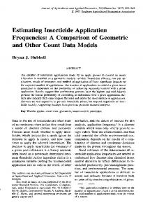
In a situation, such as ours, where the decomposition exercise is carried out across a very large number of communities, it is important to check for variation in the degree of inequality across communities. Are all communities as unequal as the country as a whole? Such a finding would certainly generate a large within-group contribution in a decomposition exercise. Or do communities vary widely in their degree of inequality? That could also yield a high within-group share. In Figures 1-5, we plot community-level inequality estimates and compare these against national-level inequality. Communities are ranked from most equal to most unequal, and 95 percent confidence intervals on each community-level estimate are included as scatter plots. Figure 1 compares parroquia level inequality in rural Ecuador against the overall inequality level in rural areas. We see that although the within-group share from the decomposition exercise was as high as 86 percent, this summary statistic masks considerable variation in parroquia inequality levels. A large majority of parroquia-level point estimates are well below the national level in rural Ecuador. Even allowing for the imprecision around the parroquia-level estimates (which are typically 5-15 percent of the point estimate), a sizeable proportion of parroquias are unambiguously more equal than the picture at the national level. Another sizeable proportion is not obviously less or more unequal than the country as a whole, and a small number of parroquias are considerably more unequal.16 In urban Ecuador (Figure 2), the proportion of zonas that have lower inequality than the national-level inequality rate is even higher than in rural areas. The precision of point estimates in urban areas of Ecuador is
16
Note the reason that there are more communities with inequality below the national level than above the national level is due to the fact that between-group inequality, while relatively small, is not absent. Differences in average per capita consumption ensure that at least some of total inequality is attributable to differences between groups. If there were no within-group inequality at all, or if all communities had the same level of within-group inequality (in the example above, suppose the eight person population were divided into two groups of four persons one with incomes 1,1,2,2, and the other with incomes 4,4,5,5) then total, national inequality would be higher than inequality in all of the individual communities (equal in the example to the common within-group inequality plus that attributable to the difference between the two groups).
20
Figure 1 Distribution across parroquias of parroquia-level inequality, rural Ecuador: GE(0)
Figure 2 Distribution across zonas of zona-level inequality, urban Ecuador: GE(0)
21
somewhat higher than in rural areas; accordingly, more zonas lie unambiguously below the national inequality level. In rural and urban Madagascar (Figures 3 and 4) and in Mozambique (Figure 5) the picture is very similar. In all of the countries considered in this study, there is a clear and sizeable subset of communities with lower inequality than the country as a whole; another large group for which inequality is not significantly different from inequality in the country as a whole; and a small third group of communities with inequality higher than the national level.
7. Correlates of Local Inequality: Does Geography Matter? We have found empirical support for both the view that at the local level, communities are more homogeneous than society as a whole, and the view that local communities are as heterogeneous as society as a whole. The question then arises as to Figure 3 Distribution across firaisanas of firaisana-level inequality, rural Madagascar: GE(0)
22
Figure 4 Distribution across firaisanas of firaisana-level inequality, urban Madagascar: GE(0)
Figure 5 Distribution across administrative posts of post-level inequality, Mozambique: GE(0)
23
whether it is possible to readily distinguish between communities on the basis of some simple indicators. In particular, we are interested to know whether there are discernable geographic patterns of inequality. In Tables 6a-6e, we provide results from OLS regressions of inequality on a set of simple community characteristics. We ask whether inequality levels are correlated with location, controlling for both demographic characteristics of the communities (population size and demographic composition), and mean per capita consumption. Table 6a for rural Ecuador finds strong evidence that inequality in the parroquias of the eastern, Oriente, region is significantly higher than the province of Pichincha in the central, mountainous, Sierra, region. Communities located in provinces in the western, coastal, Costa, region tend to be more equal, significantly so in the provinces of Manabi, Los Rios, Guayas, and El Oro. Relatively few differences are discernable across provinces within the Sierra region.17 Understanding these geographic patterns of inequality is beyond the scope of this paper, but the evidence is consistent with historical and anecdotal accounts of a very divergent evolution of society and economic structures in the mountainous Sierra vis-à-vis the Costa and Oriente.18 In rural Ecuador, there is evidence that larger parroquias tend to be more unequal. An interesting finding is that parroquias with a larger proportion of elderly, relative to the population share of 20-40-year olds, are more unequal. This pattern is consistent with the findings of Deaton and Paxson (1995) regarding the positive association between an aging population and inequality. The quantitative importance and statistical significance of both geographic and demographic characteristics remains broadly unchanged when mean per capita consumption (and its square) are added to the model. In rural Ecuador, inequality is positively associated with higher consumption levels. While there is some suggestion of a turning point (at around $2,800 per capita per month)—the
17
We can reject with 95 percent confidence, for both rural and urban Ecuador, the null hypothesis that parameter estimates on province dummies within their respective regions are all equal.
18
See, for example, “Under the Volcano,” The Economist, November 27, 1999, p. 66.
24
Table 6a Correlates of mean Log deviation (GE0) in rural Ecuador Parroquia-level regression (915 parroquias) Basic regression Log population Percent aged 0-10 Percent aged 10-20 Percent aged 40-60 Percent aged 61+ Log mean per capita expenditure (Log mean per capita expenditure)2
+ expenditure
0.0169 (0.002)*** -0.139 (0.079)* -0.375 (0.104)*** -0.246 (0.130)* 0.269 (0.123)***
0.010 (0.002)*** 0.321 (0.080)*** -0.084 (0.096) 0.053 (0.120) 0.392 (0.112)*** 0.222 (0.085)*** -0.014 (0.010)
0.036 (0.013)*** 0.051 (0.012)*** 0.071 (0.015)*** 0.040 (0.011)*** 0.034 (0.013)**
0.036 (0.012)*** 0.056 (0.011)*** 0.077 (0.013)*** 0.036 (0.010)*** 0.037 (0.012)***
Costa Esmeraldas Manabi Los Rios Guayas El Oro Galápagos
-0.012 (0.010) -0.060 (0.010)*** -0.041 (0.013)*** -0.050 (0.010)*** -0.022 (0.010)** 0.027 (0.023 )
-0.036 (0.010)*** -0.057 (0.009)*** -0.025 (0.012)** -0.035 (0.009)*** -0.020 (0.009)** -0.000 (0.021)
Sierra Carchi Imbabura Cotopaxi Tungurahua Bolivar Chimborazo Canar Azuay Loja
-0.002 (0.012) 0.024 (0.010)** -0.013 (0.011) -0.025 (0.010)** -0.0002 (0.012) -0.010 (0.010) 0.003 (0.012) 0.011 (0.010) 0.024 (0.009)**
0.014 (0.010) 0.037 (0.011)*** -0.001 (0.010) -0.010 (0.009) 0.002 (0.011) 0.006 (0.010) 0.007 (0.011) 0.014 (0.009) 0.036 (0.008)***
Oriente Sucumbios Napo Pastaza Morona_Santiago Zamora_Chinchipe
Constant Observations R-squared
0.296 (0.060) 915 0.24
-0.571 (0.192) 915 0.38
Notes: Standard errors in parentheses. * significant at 10 percent; ** significant at 5 percent. *** significant at 1 percent. Excluded groups are Pichincha and percent population age 20-40.
25
well-known “inverted U-curve”—the statistical support for this is weak. The correlation between inequality and the population share of young children, relative to 20-40-year olds, switches in sign from negative to positive, depending on whether per capita consumption is included in the specification. It seems clear that the share of young children is likely to be (negatively) correlated with per capita consumption so that the coefficient on this variable is capturing the consumption effect, when average expenditures are excluded from the specification. Once consumption expenditures are controlled for, the correlation between inequality and the share of children in the population becomes positive. Possibly there exists greater heterogeneity in household size in those parroquias with large population shares of young children and that this translates into greater inequality of per capita consumption. In urban Ecuador (Table 6b) the relatively low inequality in the Costa region is again observed. Relative to the zonas in the capital Quito, inequality in all zonas of the Costa region tends to be significantly lower. Other urban areas in the Sierra are again not noticeably less or more equal than Quito. In urban areas, in contrast to rural areas, population size of the zona does not appear to be significantly correlated with its inequality level.19 Also in contrast to rural areas, conditioning on mean consumption levels does not add much explanatory power: there is no evidence that poorer zonas are also more equal. Zonas with large dependency ratios (irrespective of whether these are due to many young children or of a large proportion of elderly) are associated with higher inequality levels, irrespective of controlling for consumption. Tables 6c and 6d provide analogous results for Madagascar. The broad conclusions are quite similar to those found in Ecuador. As in rural Ecuador, in rural Madagascar population size is positively associated with inequality, and the larger the percentage of elderly in the firaisana, the more unequal the community. As in Ecuador, inequality rises with mean consumption (in the Madagascar case the inverted U curve is more clearly
19
Although zonas vary less in population size than parroquias, they still range between 800-1,900 households.
26
Table 6b Correlates of mean Log deviation (GE0) in urban Ecuador Zona-level regression (660 zonas) Basic regression Log population Percent aged 0-10 Percent aged 10-20 Percent aged 40-60 Percent aged 61+ Log mean per capita expenditure (Log mean per capita expenditure)2
+ expenditure
-0.013 (0.015) 0.231 (0.118)* 0.283 (0.098)*** 0.001 (0.141) 0.704 (0.162)***
-0.003 (0.014) 0.253 (0.119)** 0.791 (0.112)*** -0.673 (0.162)*** 1.084 (0.161)*** 0.025 (0.075) 0.005 (0.008)
0.052 (0.033) 0.457 (0.046)*** 0.031 (0.046)
0.049 (0.031) 0.381 (0.045)*** 0.004 (0.044)
Costa Esmeraldas Manabi Los Rios Guayas El Oro Guayaquil
-0.073 (0.013)*** -0.084 (0.007)*** -0.077 (0.010)*** -0.097 (0.008)*** -0.094 (0.009)*** -0.087 (0.005 )***
-0.066 (0.012)*** -0.069 (0.007)*** -0.049 (0.011)*** -0.064 (0.008)*** -0.081 (0.009)*** -0.054 (0.007)***
Sierra Carchi Imbabura Cotopaxi Tungurahua Pichincha Chimborazo Canar Azuay Loja
-0.009 (0.017) 0.022 (0.014) 0.007 (0.016) -0.008 (0.014) -0.011 (0.010) -0.025 (0.015)* -0.012 (0.024) -0.013 (0.010) -0.003 (0.013)
0.012 (0.017) -0.008 (0.013) 0.006 (0.015) -0.003 (0.013) -0.000 (0.010) -0.026 (0.014)* -0.018 (0.022) -0.018 (0.010)* -0.010 (0.012)
Constant Observations R-squared
0.272 (0.140) 660 0.52
-0.076 (0.242) 660 0.57
Oriente Pastaza Morona_Santiago Zamora_Chinchipe
Notes: Standard errors in parentheses. * significant at 10 percent; ** significant at 5 percent. *** significant at 1 percent. Excluded groups are Quito and percent population age 20-40.
27
Table 6c Correlates of mean Log deviation (GE0) in rural Madagascar Firaisana-level regression (1,117 firaisanas) Basic regression Log population Percent aged 0-5 Percent aged 6-11 Percent aged 12-14 Percent aged 50-59 Percent aged 60+ Log mean per capita expenditure (Log mean per capita expenditure)2 Provinces Antananarivo Fianarantsoa Toamasina Mahajanga Toliara Constant Observations R-squared
+ expenditure
0.010 (0.002)*** -0.768 (0.085)*** -0.226 (0.127)* 0.193 (0.241) -1.757 (0.292)*** 0.462 (0.152)**
0.012 (0.002)*** -0.700 (0.086)*** -0.091 (0.126) 0.236 (0.242) -1.747 (0.286)*** 0.696 (0.152)*** 0.886 (0.118)*** -0.034 (0.005)***
-0.068 (0.006)*** 0.011 (0.005)** -0.059 (0.006)*** -0.115 (0.006)*** -0.046 (0.005)***
-0.065 (0.006)*** 0.020 (0.006)*** -0.054 (0.006)*** -0.116 (0.006)*** -0.042 (0.006)***
0.430 (0.041)*** 1,117 0.53
-5.356 (0.765)*** 1,117 0.55
Notes: Standard errors in parentheses. * significant at 10 percent; ** significant at 5 percent; *** significant at 1 percent. Excluded groups are Antsiranana and percent population age 15-49.
discernable) and geography is strongly and independently significant. Relative to the population share aged 15-50, the higher the share of children and the share of population aged 50-59, the more equal the community, whether or not one controls for consumption. In Madagascar, it seems that communities with large population shares of children are not markedly more heterogeneous in household size. For rural Madagascar, the simple specification employed here yields an R2 as high as 0.55 when all variables are included. In urban Madagascar, the explanatory power is even greater (Table 6d). Here, unlike rural areas, population size is significantly negatively associated with inequality. As in rural areas, the larger the percentage of children, the lower is inequality. As in urban Ecuador, mean per capita consumption is not significantly associated with inequality—there is no presumption that a poorer urban firaisana is more homogeneous than a rich one. Geographic variables remain independently significant, with urban areas in Antananarivo
28
Table 6d Correlates of mean Log deviation (GE0) in urban Madagascar Firaisana-level regression (131 firaisanas) Basic regression Log population Percent aged 0-5 Percent aged 6-11 Percent aged 12-14 Percent aged 50-59 Percent aged 60+ Log mean per capita expenditure (Log mean per capita expenditure)2 Provinces Antananarivo Fianarantsoa Toamasina Mahajanga Toliara Constant Observations R-squared
+ expenditure
-0.014 (0.005)*** -1.253 (0.202)*** 0.166 (0.464) -0.965 (0.777) -2.602 (0.882)*** 1.183 (0.396)***
-0.011 (0.005)** -1.053 (0.243)*** 0.147 (0.465) -0.551 (0.826) -2.543 (0.882)*** 1.355 (0.417)*** 0.117 (0.143) -0.004 (0.013)
0.079 (0.015)*** 0.059 (0.014)*** -0.012 (0.014) -0.025 (0.014)* 0.117 (0.013)***
0.080 (0.015)*** 0.065 (0.015)*** -0.007 (0.015) -0.027 (0.014)* 0.125 (0.014)***
0.717 (0.106) 131 0.78
-0.270 (2.245) 131 0.79
Notes: Standard errors in parentheses. * significant at 10 percent; ** significant at 5 percent; *** significant at 1 percent. Excluded groups are Antsiranana and and population age 15-49.
(the capital province), Fianarantsoa, and Toliara more unequal than the urban areas in the rest of the country. Table 6e confirms that in Mozambique, too, geographic variables are key indicators of local-level inequality, controlling for population characteristics, mean expenditure levels, and urban/rural differences. Compared with Maputo City, the rest of the country has significantly less inequality. There is more inequality in urban areas, an increasing association with mean consumption (but no Kuznets curve), and areas with a higher percentage of 17-30-year-olds seem to have higher inequality. We have not attempted here to identify the best possible set of correlates of local inequality for each of the three countries we are examining. We have chosen to employ a parsimonious, and broadly similar, specification in the three countries in order to ask whether there are any common patterns across countries that in other respects resemble
29
Table 6e Correlates of mean Log deviation (GE0) in Mozambique Administrative post-level regression (464 administrative posts) Basic regression
+ expenditure
+ urban
Percent aged 0-5 Percent aged 6-10 Percent females aged 11-16 Percent males aged 11-16 Percent females aged 17-30 Percent males aged 17-30 Percent females aged 31-60 Percent males aged 31-60 Log (population of posto) Niassa Cabo Delgado Nampula Zambézia Tete Manica Sofala Inhambane Gaza Maputo Province Log (mean expenditure) [Log (mean expenditure)]squared Urban
-0.002 (0.004) 0.017 (0.005)** 0.027 (0.009)** -0.000 (0.009) 0.016** (0.004) 0.015 (0.005)** 0.005 (0.006) 0.007 (0.004) 0.001 (0.004) -0.200 (0.036)** -0.204 (0.034)** -0.204 (0.035)** -0.215 (0.035)** -0.212 (0.036)** -0.135 (0.035)** -0.118 (0.035)** -0.178 (0.035)** -0.189 (0.035)** -0.088 (0.036)*
0.000 (0.003) 0.015 (0.004)** 0.020 (0.008)** 0.001 (0.008) 0.012 (0.003)** 0.010 (0.004)* 0.005 (0.006) 0.005 (0.004) -0.003 (0.003) -0.138 (0.034)** -0.163 (0.031)** -0.143 (0.032)** -0.154 (0.032)** -0.133 (0.033)** -0.095 (0.032)** -0.005 (0.032) -0.088 (0.032)** -0.136 (0.032)** -0.045 (0.032) -0.406 (0.216) 0.031 (0.013)*
0.001 (0.003) 0.014 (0.004)** 0.015 (0.008) 0.002 (0.008) 0.011 (0.003)** 0.009 (0.004)* 0.007 (0.006) 0.004 (0.004) -0.005 (0.004) -0.136 (0.033)** -0.158 (0.031)** -0.143 (0.032)** -0.149 (0.032)** -0.127 (0.033)** -0.089 (0.032)** -0.006 (0.032) -0.090 (0.032)** -0.135 (0.031)** -0.044 (0.032) -0.324 (0.217) 0.025 (0.013)* 0.037 (0.014)**
Constant Observations R-squared
-0.504 (0.321) 424 0.465
0.856 (0.962) 424 0.595
0.605 (0.960) 424 0.601
Notes: Standard errors in parentheses. * significant at 5 percent; ** significant at 1 percent. Excluded groups are Maputo city and percent persons older than 60 years.
each other very little (particularly the comparison between Ecuador and the two SubSaharan African countries). We have indeed found that in all three countries we consider, in both rural and urban areas, geographic location is a good predictor of locallevel inequality, even after controlling for some basic demographic and economic characteristics of the communities. With respect to other characteristics, there appear to be clear differences between urban and rural areas (best seen in the models for Ecuador
30
and Madagascar). In rural areas, inequality tends to be higher in communities with larger populations, a higher share of the elderly in the total population, and in communities with higher mean consumption levels. In urban areas, mean consumption is not independently correlated with inequality, and inequality is not typically higher in communities with larger populations. High population shares of elderly are clearly associated with higher inequality, but the correlation with population shares of children depends on the country.
8. Conclusions This paper has taken three developing countries, Ecuador, Madagascar, and Mozambique, and has implemented in each a methodology to produce disaggregated estimates of inequality. The countries are very unlike each other—with different geographies, stages of development, quality and types of data, and so on. The methodology works well in all three settings and produces valuable information about the spatial distribution of poverty and inequality within those countries—information that was previously not available. The methodology is based on a statistical procedure to combine household survey data with population census data, by imputing into the latter a measure of economic welfare (consumption expenditure in our examples) from the former. Like the usual sample-based estimates, the inequality measures produced are also estimates and subject to statistical error. The paper has demonstrated that the mean consumption, poverty, and inequality estimates produced from census data match well the estimates calculated directly from the country’s surveys (at levels of disaggregation that the survey can bear). The precision of the inequality estimates produced with this methodology depends on the degree of disaggregation. In all three countries considered here, our inequality estimators allow one to work at a level of disaggregation far below that allowed by surveys. We have decomposed inequality in our three countries into progressively more disaggregated spatial units, and have shown that even at a very high level of spatial disaggregation, the contribution to overall inequality of within-community inequality is
31
very high (75 percent or more). We have argued that such a high within-group component does not necessarily imply that there are no between-group differences at all and that all communities in a given country are as unequal as the country as a whole. We have shown that in all three countries, there is a considerable amount of variation in inequality across communities. Many communities are rather more equal than their respective country as a whole, but there are also many communities that are not clearly more homogeneous than society as a whole, and may even be considerably more unequal. We have explored some basic correlates of local-level inequality in our three countries. We have found consistent patterns across all three countries. Geographic characteristics are strongly correlated with inequality, even after controlling for demographic and economic conditions. The correlation with geography is observed in both rural and urban areas. In rural areas, population size and mean consumption at the community level are positively associated with inequality, while in urban areas that is not the case. In both rural and urban areas, populations with large shares of the elderly tend to be more unequal. In Madagascar, populations with large shares of children and large shares of individuals aged 50-59 are consistently more equal. In Ecuador, this is true only in rural areas.
32
References Atkinson, A. B., and F. Bourguignon. 2000. Introduction: Income distribution and economics. In Handbook of income distribution, Vol. 1, ed. A. B. Atkinson and E. Bourguignon. North Holland: Elsevier Science, B.V. Bardhan, P., and D. Mookherjee. 1999. Relative capture of local and central governments. Boston, Mass., U.S.A.: Boston University. Bourguignon, F. 1979. Decomposable income inequality measures. Econometrica 47 (4): 901-920. Cowell, F. 1980. On the structure of additive inequality measures. Review of Economic Studies 47: 521-531. Cowell, F. 2000. Measurement of inequality. In Handbook of income distribution, Vol. 1, ed. A. B. Atkinson and E. Bourguignon. North Holland: Elsevier Science, B.V. Datt, G., K. Simler, S. Mukherjee, and G. Dava. 2000. Determinants of poverty in Mozambique, 1996-97. Food Consumption and Nutrition Division Discussion Paper 78. Washington, D.C.: International Food Policy Research Institute. Deaton, A. 1999. Inequalities in income and in health. Working Papers No. 7141. Cambridge, Mass., U.S.A.: National Bureau of Economic Research. Deaton. A., and C. Paxson. 1995. Savings, inequality and aging: An East Asian perspective. Asia-Pacific Economic Review. Demombynes, G., C. Elbers, J. O. Lanjouw, P. Lanjouw, J. Mistiaen, and B. Özler. 2002. Producing an improved geographic profile of poverty: Methodology and evidence from three developing countries. Discussion Paper 2002/39. Helsinki: WIDER. Elbers, C., J. O. Lanjouw, and P. Lanjouw. 2000. Welfare in villages and towns: Microlevel estimation of poverty and inequality. Working Paper No. 2000-029/2. Amsterdam: Tinbergen Institute.
33
Elbers, C., J. O. Lanjouw, and P. Lanjouw. 2002. Micro-level estimation of welfare. Policy Research Working Paper 2911. Washington, D.C.: Development Research Group, World Bank. Elbers, C., J. O. Lanjouw, and P. Lanjouw. 2003. Micro-level estimation of poverty and inequality. Econometrica 71 (1): 355-364. Elbers, C., J. O. Lanjouw, P. Lanjouw, and P. G. Leite. 2001. Poverty and inequality in Brazil: New estimates from combined PPV-PNAD Data. DECRG-World Bank, Washington, D.C. Photocopy. Galasso, E., and M. Ravallion. 2002. Decentralized targeting of an anti-poverty program. DECRG-World Bank, Washington, D.C. Photocopy. Hentschel, J., and P. Lanjouw. 1996. Constructing an indicator of consumption for the analysis of poverty: Principles and illustrations with reference to Ecuador. LSMS Working Paper No. 124. Washington, D.C.: DECRG-World Bank. Hentschel, J., J. O. Lanjouw, P. Lanjouw, and J. Poggi. 2000. Combining census and survey data to trace the spatial dimensions of poverty: A case study of Ecuador. World Bank Economic Review 14 (1): 147-165. Kanbur, R. 2000. Income distribution and development. In Handbook of income distribution, Vol. 1, ed. A. B. Atkinson and E. Bourguignon. North Holland: Elsevier Science, B.V. Lanjouw, P., and N. Stern. 1998. Economic development in Palanpur over five decades. Oxford: Oxford University Press. Mistiaen, J., B. Özler, T. Razafimanantena, and J. Razafindravonona. 2002. Putting welfare on the map in Madagascar. DECRG-World Bank, Washington, D.C. Photocopy. Ravallion, M. 1999. Is more targeting consistent with less spending? International Tax and Public Finance 6 (3): 411-419. Ravallion, M. 2000. Monitoring targeting performance when decentralized allocations to the poor are unobserved. World Bank Economic Review 14 (2): 331-345.
34
Sen, A., and J. Foster. 1997. On economic inequality. 2nd edition. Oxford: Oxford University Press. Shorrocks, A. 1980. The class of additively decomposable inequality measures. Econometrica 48 (3): 613-625. Simler, K., and V. Nhate. 2002. Poverty, inequality and geographic targeting: Evidence from small-area estimates in Mozambique. International Food Policy Research Institute, Washington, D.C. Photocopy. Tendler, J. 1997. Good government in the tropics. Baltimore, Md., U.S.A.: Johns Hopkins University Press. World Bank. 1996. Ecuador poverty report. In World Bank country study. Washington, D.C.: Ecuador Country Department, World Bank.
FCND DISCUSSION PAPERS 146
Moving Forward with Complementary Feeding: Indicators and Research Priorities, Marie T. Ruel, Kenneth H. Brown, and Laura E. Caulfield, April 2003
145
Child Labor and School Decisions in Urban and Rural Areas: Cross Country Evidence, Lire Ersado, December 2002
144
Targeting Outcomes Redux, David Coady, Margaret Grosh, and John Hoddinott, December 2002
143
Progress in Developing an Infant and Child Feeding Index: An Example Using the Ethiopia Demographic and Health Survey 2000, Mary Arimond and Marie T. Ruel, December 2002
142
Social Capital and Coping With Economic Shocks: An Analysis of Stunting of South African Children, Michael R. Carter and John A. Maluccio, December 2002
141
The Sensitivity of Calorie-Income Demand Elasticity to Price Changes: Evidence from Indonesia, Emmanuel Skoufias, November 2002
140
Is Dietary Diversity an Indicator of Food Security or Dietary Quality? A Review of Measurement Issues and Research Needs, Marie T. Ruel, November 2002
139
Can South Africa Afford to Become Africa’s First Welfare State? James Thurlow, October 2002
138
The Food for Education Program in Bangladesh: An Evaluation of its Impact on Educational Attainment and Food Security, Akhter U. Ahmed and Carlo del Ninno, September 2002
137
Reducing Child Undernutrition: How Far Does Income Growth Take Us? Lawrence Haddad, Harold Alderman, Simon Appleton, Lina Song, and Yisehac Yohannes, August 2002
136
Dietary Diversity as a Food Security Indicator, John Hoddinott and Yisehac Yohannes, June 2002
135
Trust, Membership in Groups, and Household Welfare: Evidence from KwaZulu-Natal, South Africa, Lawrence Haddad and John A. Maluccio, May 2002
134
In-Kind Transfers and Household Food Consumption: Implications for Targeted Food Programs in Bangladesh, Carlo del Ninno and Paul A. Dorosh, May 2002
133
Avoiding Chronic and Transitory Poverty: Evidence From Egypt, 1997-99, Lawrence Haddad and Akhter U. Ahmed, May 2002
132
Weighing What’s Practical: Proxy Means Tests for Targeting Food Subsidies in Egypt, Akhter U. Ahmed and Howarth E. Bouis, May 2002
131
Does Subsidized Childcare Help Poor Working Women in Urban Areas? Evaluation of a GovernmentSponsored Program in Guatemala City, Marie T. Ruel, Bénédicte de la Brière, Kelly Hallman, Agnes Quisumbing, and Nora Coj, April 2002
130
Creating a Child Feeding Index Using the Demographic and Health Surveys: An Example from Latin America, Marie T. Ruel and Purnima Menon, April 2002
129
Labor Market Shocks and Their Impacts on Work and Schooling: Evidence from Urban Mexico, Emmanuel Skoufias and Susan W. Parker, March 2002
128
Assessing the Impact of Agricultural Research on Poverty Using the Sustainable Livelihoods Framework, Michelle Adato and Ruth Meinzen-Dick, March 2002
127
A Cost-Effectiveness Analysis of Demand- and Supply-Side Education Interventions: The Case of PROGRESA in Mexico, David P. Coady and Susan W. Parker, March 2002
126
Health Care Demand in Rural Mozambique: Evidence from the 1996/97 Household Survey, Magnus Lindelow, February 2002
125
Are the Welfare Losses from Imperfect Targeting Important?, Emmanuel Skoufias and David Coady, January 2002
124
The Robustness of Poverty Profiles Reconsidered, Finn Tarp, Kenneth Simler, Cristina Matusse, Rasmus Heltberg, and Gabriel Dava, January 2002
123
Conditional Cash Transfers and Their Impact on Child Work and Schooling: Evidence from the PROGRESA Program in Mexico, Emmanuel Skoufias and Susan W. Parker, October 2001
FCND DISCUSSION PAPERS 122
Strengthening Public Safety Nets: Can the Informal Sector Show the Way?, Jonathan Morduch and Manohar Sharma, September 2001
121
Targeting Poverty Through Community-Based Public Works Programs: A Cross-Disciplinary Assessment of Recent Experience in South Africa, Michelle Adato and Lawrence Haddad, August 2001
120
Control and Ownership of Assets Within Rural Ethiopian Households, Marcel Fafchamps and Agnes R. Quisumbing, August 2001
119
Assessing Care: Progress Towards the Measurement of Selected Childcare and Feeding Practices, and Implications for Programs, Mary Arimond and Marie T. Ruel, August 2001
118
Is PROGRESA Working? Summary of the Results of an Evaluation by IFPRI, Emmanuel Skoufias and Bonnie McClafferty, July 2001
117
Evaluation of the Distributional Power of PROGRESA’s Cash Transfers in Mexico, David P. Coady, July 2001
116
A Multiple-Method Approach to Studying Childcare in an Urban Environment: The Case of Accra, Ghana, Marie T. Ruel, Margaret Armar-Klemesu, and Mary Arimond, June 2001
115
Are Women Overrepresented Among the Poor? An Analysis of Poverty in Ten Developing Countries, Agnes R. Quisumbing, Lawrence Haddad, and Christina Peña, June 2001
114
Distribution, Growth, and Performance of Microfinance Institutions in Africa, Asia, and Latin America, Cécile Lapenu and Manfred Zeller, June 2001
113
Measuring Power, Elizabeth Frankenberg and Duncan Thomas, June 2001
112
Effective Food and Nutrition Policy Responses to HIV/AIDS: What We Know and What We Need to Know, Lawrence Haddad and Stuart Gillespie, June 2001
111
An Operational Tool for Evaluating Poverty Outreach of Development Policies and Projects, Manfred Zeller, Manohar Sharma, Carla Henry, and Cécile Lapenu, June 2001
110
Evaluating Transfer Programs Within a General Equilibrium Framework, Dave Coady and Rebecca Lee Harris, June 2001
109
Does Cash Crop Adoption Detract From Childcare Provision? Evidence From Rural Nepal, Michael J. Paolisso, Kelly Hallman, Lawrence Haddad, and Shibesh Regmi, April 2001
108
How Efficiently Do Employment Programs Transfer Benefits to the Poor? Evidence from South Africa, Lawrence Haddad and Michelle Adato, April 2001
107
Rapid Assessments in Urban Areas: Lessons from Bangladesh and Tanzania, James L. Garrett and Jeanne Downen, April 2001
106
Strengthening Capacity to Improve Nutrition, Stuart Gillespie, March 2001
105
The Nutritional Transition and Diet-Related Chronic Diseases in Asia: Implications for Prevention, Barry M. Popkin, Sue Horton, and Soowon Kim, March 2001
104
An Evaluation of the Impact of PROGRESA on Preschool Child Height, Jere R. Behrman and John Hoddinott, March 2001
103
Targeting the Poor in Mexico: An Evaluation of the Selection of Households for PROGRESA, Emmanuel Skoufias, Benjamin Davis, and Sergio de la Vega, March 2001
102
School Subsidies for the Poor: Evaluating a Mexican Strategy for Reducing Poverty, T. Paul Schultz, March 2001
101
Poverty, Inequality, and Spillover in Mexico’s Education, Health, and Nutrition Program, Sudhanshu Handa, Mari-Carmen Huerta, Raul Perez, and Beatriz Straffon, March 2001
100
On the Targeting and Redistributive Efficiencies of Alternative Transfer Instruments, David Coady and Emmanuel Skoufias, March 2001
99
Cash Transfer Programs with Income Multipliers: PROCAMPO in Mexico, Elisabeth Sadoulet, Alain de Janvry, and Benjamin Davis, January 2001
FCND DISCUSSION PAPERS 98
Participation and Poverty Reduction: Issues, Theory, and New Evidence from South Africa, John Hoddinott, Michelle Adato, Tim Besley, and Lawrence Haddad, January 2001
97
Socioeconomic Differentials in Child Stunting Are Consistently Larger in Urban Than in Rural Areas, Purnima Menon, Marie T. Ruel, and Saul S. Morris, December 2000
96
Attrition in Longitudinal Household Survey Data: Some Tests for Three Developing-Country Samples, Harold Alderman, Jere R. Behrman, Hans-Peter Kohler, John A. Maluccio, Susan Cotts Watkins, October 2000
95
Attrition in the Kwazulu Natal Income Dynamics Study 1993-1998, John Maluccio, October 2000
94
Targeting Urban Malnutrition: A Multicity Analysis of the Spatial Distribution of Childhood Nutritional Status, Saul Sutkover Morris, September 2000
93
Mother-Father Resource Control, Marriage Payments, and Girl-Boy Health in Rural Bangladesh, Kelly K. Hallman, September 2000
92
Assessing the Potential for Food-Based Strategies to Reduce Vitamin A and Iron Deficiencies: A Review of Recent Evidence, Marie T. Ruel and Carol E. Levin, July 2000
91
Comparing Village Characteristics Derived From Rapid Appraisals and Household Surveys: A Tale From Northern Mali, Luc Christiaensen, John Hoddinott, and Gilles Bergeron, July 2000
90
Empirical Measurements of Households’ Access to Credit and Credit Constraints in Developing Countries: Methodological Issues and Evidence, Aliou Diagne, Manfred Zeller, and Manohar Sharma, July 2000
89
The Role of the State in Promoting Microfinance Institutions, Cécile Lapenu, June 2000
88
The Determinants of Employment Status in Egypt, Ragui Assaad, Fatma El-Hamidi, and Akhter U. Ahmed, June 2000
87
Changes in Intrahousehold Labor Allocation to Environmental Goods Collection: A Case Study from Rural Nepal, Priscilla A. Cooke, May 2000
86
Women’s Assets and Intrahousehold Allocation in Rural Bangladesh: Testing Measures of Bargaining Power, Agnes R. Quisumbing and Bénédicte de la Brière, April 2000
85
Intrahousehold Impact of Transfer of Modern Agricultural Technology: A Gender Perspective, Ruchira Tabassum Naved, April 2000
84
Intrahousehold Allocation and Gender Relations: New Empirical Evidence from Four Developing Countries, Agnes R. Quisumbing and John A. Maluccio, April 2000
83
Quality or Quantity? The Supply-Side Determinants of Primary Schooling in Rural Mozambique, Sudhanshu Handa and Kenneth R. Simler, March 2000
82
Pathways of Rural Development in Madagascar: An Empirical Investigation of the Critical Triangle of Environmental Sustainability, Economic Growth, and Poverty Alleviation, Manfred Zeller, Cécile Lapenu, Bart Minten, Eliane Ralison, Désiré Randrianaivo, and Claude Randrianarisoa, March 2000
81
The Constraints to Good Child Care Practices in Accra: Implications for Programs, Margaret ArmarKlemesu, Marie T. Ruel, Daniel G. Maxwell, Carol E. Levin, and Saul S. Morris, February 2000
80
Nontraditional Crops and Land Accumulation Among Guatemalan Smallholders: Is the Impact Sustainable? Calogero Carletto, February 2000
79
Adult Health in the Time of Drought, John Hoddinott and Bill Kinsey, January 2000
78
Determinants of Poverty in Mozambique: 1996-97, Gaurav Datt, Kenneth Simler, Sanjukta Mukherjee, and Gabriel Dava, January 2000
77
The Political Economy of Food Subsidy Reform in Egypt, Tammi Gutner, November 1999.
76
Raising Primary School Enrolment in Developing Countries: The Relative Importance of Supply and Demand, Sudhanshu Handa, November 1999
75
Determinants of Poverty in Egypt, 1997, Gaurav Datt and Dean Jolliffe, October 1999
74
Can Cash Transfer Programs Work in Resource-Poor Countries? The Experience in Mozambique, Jan W. Low, James L. Garrett, and Vitória Ginja, October 1999
FCND DISCUSSION PAPERS 73
Social Roles, Human Capital, and the Intrahousehold Division of Labor: Evidence from Pakistan, Marcel Fafchamps and Agnes R. Quisumbing, October 1999
72
Validity of Rapid Estimates of Household Wealth and Income for Health Surveys in Rural Africa, Saul S. Morris, Calogero Carletto, John Hoddinott, and Luc J. M. Christiaensen, October 1999
71
Social Capital and Income Generation in South Africa, 1993-98, John Maluccio, Lawrence Haddad, and Julian May, September 1999
70
Child Health Care Demand in a Developing Country: Unconditional Estimates from the Philippines, Kelly Hallman, August 1999
69
Supply Response of West African Agricultural Households: Implications of Intrahousehold Preference Heterogeneity, Lisa C. Smith and Jean-Paul Chavas, July 1999
68
Early Childhood Nutrition and Academic Achievement: A Longitudinal Analysis, Paul Glewwe, Hanan Jacoby, and Elizabeth King, May 1999
67
Determinants of Household Access to and Participation in Formal and Informal Credit Markets in Malawi, Aliou Diagne, April 1999
66
Working Women in an Urban Setting: Traders, Vendors, and Food Security in Accra, Carol E. Levin, Daniel G. Maxwell, Margaret Armar-Klemesu, Marie T. Ruel, Saul S. Morris, and Clement Ahiadeke, April 1999
65
Are Determinants of Rural and Urban Food Security and Nutritional Status Different? Some Insights from Mozambique, James L. Garrett and Marie T. Ruel, April 1999
64
Some Urban Facts of Life: Implications for Research and Policy, Marie T. Ruel, Lawrence Haddad, and James L. Garrett, April 1999
63
Are Urban Poverty and Undernutrition Growing? Some Newly Assembled Evidence, Lawrence Haddad, Marie T. Ruel, and James L. Garrett, April 1999
62
Good Care Practices Can Mitigate the Negative Effects of Poverty and Low Maternal Schooling on Children's Nutritional Status: Evidence from Accra, Marie T. Ruel, Carol E. Levin, Margaret ArmarKlemesu, Daniel Maxwell, and Saul S. Morris, April 1999
61
Does Geographic Targeting of Nutrition Interventions Make Sense in Cities? Evidence from Abidjan and Accra, Saul S. Morris, Carol Levin, Margaret Armar-Klemesu, Daniel Maxwell, and Marie T. Ruel, April 1999
60
Explaining Child Malnutrition in Developing Countries: A Cross-Country Analysis, Lisa C. Smith and Lawrence Haddad, April 1999
59
Placement and Outreach of Group-Based Credit Organizations: The Cases of ASA, BRAC, and PROSHIKA in Bangladesh, Manohar Sharma and Manfred Zeller, March 1999
58
Women's Land Rights in the Transition to Individualized Ownership: Implications for the Management of Tree Resources in Western Ghana, Agnes Quisumbing, Ellen Payongayong, J. B. Aidoo, and Keijiro Otsuka, February 1999
57
The Structure of Wages During the Economic Transition in Romania, Emmanuel Skoufias, February 1999
56
How Does the Human Rights Perspective Help to Shape the Food and Nutrition Policy Research Agenda?, Lawrence Haddad and Arne Oshaug, February 1999
55
Efficiency in Intrahousehold Resource Allocation, Marcel Fafchamps, December 1998
54
Endogeneity of Schooling in the Wage Function: Evidence from the Rural Philippines, John Maluccio, November 1998
53
Agricultural Wages and Food Prices in Egypt: A Governorate-Level Analysis for 1976-1993, Gaurav Datt and Jennifer Olmsted, November 1998
52
Testing Nash Bargaining Household Models With Time-Series Data, John Hoddinott and Christopher Adam, November 1998
FCND DISCUSSION PAPERS 51
Urban Challenges to Food and Nutrition Security: A Review of Food Security, Health, and Caregiving in the Cities, Marie T. Ruel, James L. Garrett, Saul S. Morris, Daniel Maxwell, Arne Oshaug, Patrice Engle, Purnima Menon, Alison Slack, and Lawrence Haddad, October 1998
50
Computational Tools for Poverty Measurement and Analysis, Gaurav Datt, October 1998
49
A Profile of Poverty in Egypt: 1997, Gaurav Datt, Dean Jolliffe, and Manohar Sharma, August 1998.
48
Human Capital, Productivity, and Labor Allocation in Rural Pakistan, Marcel Fafchamps and Agnes R. Quisumbing, July 1998
47
Poverty in India and Indian States: An Update, Gaurav Datt, July 1998
46
Impact of Access to Credit on Income and Food Security in Malawi, Aliou Diagne, July 1998
45
Does Urban Agriculture Help Prevent Malnutrition? Evidence from Kampala, Daniel Maxwell, Carol Levin, and Joanne Csete, June 1998
44
Can FAO's Measure of Chronic Undernourishment Be Strengthened?, Lisa C. Smith, with a Response by Logan Naiken, May 1998
43
How Reliable Are Group Informant Ratings? A Test of Food Security Rating in Honduras, Gilles Bergeron, Saul Sutkover Morris, and Juan Manuel Medina Banegas, April 1998
42
Farm Productivity and Rural Poverty in India, Gaurav Datt and Martin Ravallion, March 1998
41
The Political Economy of Urban Food Security in Sub-Saharan Africa, Dan Maxwell, February 1998
40
Can Qualitative and Quantitative Methods Serve Complementary Purposes for Policy Research? Evidence from Accra, Dan Maxwell, January 1998
39
Whose Education Matters in the Determination of Household Income: Evidence from a Developing Country, Dean Jolliffe, November 1997
38
Systematic Client Consultation in Development: The Case of Food Policy Research in Ghana, India, Kenya, and Mali, Suresh Chandra Babu, Lynn R. Brown, and Bonnie McClafferty, November 1997
37
Why Do Migrants Remit? An Analysis for the Dominican Sierra, Bénédicte de la Brière, Alain de Janvry, Sylvie Lambert, and Elisabeth Sadoulet, October 1997
36
The GAPVU Cash Transfer Program in Mozambique: An assessment, Gaurav Datt, Ellen Payongayong, James L. Garrett, and Marie Ruel, October 1997
35
Market Access by Smallholder Farmers in Malawi: Implications for Technology Adoption, Agricultural Productivity, and Crop Income, Manfred Zeller, Aliou Diagne, and Charles Mataya, September 1997
34
The Impact of Changes in Common Property Resource Management on Intrahousehold Allocation, Philip Maggs and John Hoddinott, September 1997
33
Human Milk—An Invisible Food Resource, Anne Hatløy and Arne Oshaug, August 1997
32
The Determinants of Demand for Micronutrients: An Analysis of Rural Households in Bangladesh, Howarth E. Bouis and Mary Jane G. Novenario-Reese, August 1997
31
Is There an Intrahousehold 'Flypaper Effect'? Evidence from a School Feeding Program, Hanan Jacoby, August 1997
30
Plant Breeding: A Long-Term Strategy for the Control of Zinc Deficiency in Vulnerable Populations, Marie T. Ruel and Howarth E. Bouis, July 1997
29
Gender, Property Rights, and Natural Resources, Ruth Meinzen-Dick, Lynn R. Brown, Hilary Sims Feldstein, and Agnes R. Quisumbing, May 1997
28
Developing a Research and Action Agenda for Examining Urbanization and Caregiving: Examples from Southern and Eastern Africa, Patrice L. Engle, Purnima Menon, James L. Garrett, and Alison Slack, April 1997
27
"Bargaining" and Gender Relations: Within and Beyond the Household, Bina Agarwal, March 1997
FCND DISCUSSION PAPERS 26
Why Have Some Indian States Performed Better Than Others at Reducing Rural Poverty?, Gaurav Datt and Martin Ravallion, March 1997
25
Water, Health, and Income: A Review, John Hoddinott, February 1997
24
Child Care Practices Associated with Positive and Negative Nutritional Outcomes for Children in Bangladesh: A Descriptive Analysis, Shubh K. Kumar Range, Ruchira Naved, and Saroj Bhattarai, February 1997
23
Better Rich, or Better There? Grandparent Wealth, Coresidence, and Intrahousehold Allocation, Agnes R. Quisumbing, January 1997
22
Alternative Approaches to Locating the Food Insecure: Qualitative and Quantitative Evidence from South India, Kimberly Chung, Lawrence Haddad, Jayashree Ramakrishna, and Frank Riely, January 1997
21
Livestock Income, Male/Female Animals, and Inequality in Rural Pakistan, Richard H. Adams, Jr., November 1996
20
Macroeconomic Crises and Poverty Monitoring: A Case Study for India, Gaurav Datt and Martin Ravallion, November 1996
19
Food Security and Nutrition Implications of Intrahousehold Bias: A Review of Literature, Lawrence Haddad, Christine Peña, Chizuru Nishida, Agnes Quisumbing, and Alison Slack, September 1996
18
Care and Nutrition: Concepts and Measurement, Patrice L. Engle, Purnima Menon, and Lawrence Haddad, August 1996
17
Remittances, Income Distribution, and Rural Asset Accumulation, Richard H. Adams, Jr., August 1996
16
How Can Safety Nets Do More with Less? General Issues with Some Evidence from Southern Africa, Lawrence Haddad and Manfred Zeller, July 1996
15
Repayment Performance in Group-Based credit Programs in Bangladesh: An Empirical Analysis, Manohar Sharma and Manfred Zeller, July 1996
14
Demand for High-Value Secondary Crops in Developing Countries: The Case of Potatoes in Bangladesh and Pakistan, Howarth E. Bouis and Gregory Scott, May 1996
13
Determinants of Repayment Performance in Credit Groups: The Role of Program Design, Intra-Group Risk Pooling, and Social Cohesion in Madagascar, Manfred Zeller, May 1996
12
Child Development: Vulnerability and Resilience, Patrice L. Engle, Sarah Castle, and Purnima Menon, April 1996
11
Rural Financial Policies for Food Security of the Poor: Methodologies for a Multicountry Research Project, Manfred Zeller, Akhter Ahmed, Suresh Babu, Sumiter Broca, Aliou Diagne, and Manohar Sharma, April 1996
10
Women's Economic Advancement Through Agricultural Change: A Review of Donor Experience, Christine Peña, Patrick Webb, and Lawrence Haddad, February 1996
09
Gender and Poverty: New Evidence from 10 Developing Countries, Agnes R. Quisumbing, Lawrence Haddad, and Christine Peña, December 1995
08
Measuring Food Insecurity: The Frequency and Severity of "Coping Strategies," Daniel G. Maxwell, December 1995
07
A Food Demand System Based on Demand for Characteristics: If There Is "Curvature" in the Slutsky Matrix, What Do the Curves Look Like and Why?, Howarth E. Bouis, December 1995
06
Gender Differentials in Farm Productivity: Implications for Household Efficiency and Agricultural Policy, Harold Alderman, John Hoddinott, Lawrence Haddad, and Christopher Udry, August 1995
05
Gender Differences in Agricultural Productivity: A Survey of Empirical Evidence, Agnes R. Quisumbing, July 1995
04
Market Development and Food Demand in Rural China, Jikun Huang and Scott Rozelle, June 1995
FCND DISCUSSION PAPERS 03
The Extended Family and Intrahousehold Allocation: Inheritance and Investments in Children in the Rural Philippines, Agnes R. Quisumbing, March 1995
02
Determinants of Credit Rationing: A Study of Informal Lenders and Formal Credit Groups in Madagascar, Manfred Zeller, October 1994
01
Agricultural Technology and Food Policy to Combat Iron Deficiency in Developing Countries, Howarth E. Bouis, August 1994