Arrays in a Lazy Functional Language – a case study: the ... - CiteSeerX

Arrays in a Lazy Functional Language – a case study: the Fast Fourier Transform Pieter H. Hartel and Willem G. Vree Department of Computer Systems University of Amsterdam Kruislaan 403, 1098 SJ Amsterdam, The Netherlands

Abstract The array plays a prominent role in imperative programming languages because the data structure bears a close resemblance to the mathematical notion of a vector and because array operations can be implemented efficiently. Not all lazy functional languages offer arrays as a primitive data structure because laziness makes it difficult to implement arrays efficiently. We study 8 different versions of the Fast Fourier Transform, with and without arrays, to assess the importance of arrays in a lazy functional language. An efficient implementation of arrays contributes significantly to the performance of functional languages in certain areas. However, a clear distinction should be made between array construction and array subscription. In the FFT example we could not gain efficiency by using array construction, other than for storing precomputed data like the input. Using array subscription improves performance.

1 Introduction Lazy functional languages like Haskell [8] and Tale [1] offer lazy linear arrays as a primitive data structure as well as a set of built in functions to operate on such arrays. Other languages, such as Miranda [11] do not provide arrays. The data structure that comes naturally with (lazy) functional languages is the list. It is essentially a linear structure, like the array, but is built up piecemeal, rather than in one step. Building an array in one step allows the compiler to generate index calculations, which make random access of array elements possible in constant time. Because lists are constructed piecemeal, random access in constant time is generally not possible with elements of lists. This difference gives arrays an efficiency advantage over lists in a lazy functional language. When building a lazy array, the elements are not necessarily evaluated. In this respect there is no performance difference between arrays and lists. The performance of an array becomes equal to that of a list when the elements are selected in index order 1; 2; : : : which is the case for many vector and matrix operations. To study the advantages of arrays, we must thus look for applications that consume array elements in some other order than in which the elements are produced. This restricts the class of algorithms for which arrays are intrinsically better suitable than lists. It is difficult to make good use of arrays because it is usually more expensive to create an array than it is to create a list (see below). To compensate for the cost of creation, it may be necessary to traverse the data structure twice, or even more often, in non index order, for the array to break even with the list. To contrast the efficiency of linear array primitives with comparable list operations, we assume naive but realistic implementations of both. For lists this amounts to a linked list of 1

cons cells and we assume that each array creating primitive allocates one block of memory large enough to store (pointers to) all lazy array elements. Array subscription requires O(1) time, while list projection takes O(n) time. In a sophisticated implementation of arrays and lists, destructive update of aggregates allows for a considerable improvement in performance with respect to a naive implementation [2]. Our compiler does not perform update analysis, but fortunately this facility is not needed by any of the Fast Fourier Transform (FFT) versions used in our case study. Arrays of dimension 2 or higher are not considered here because the FFT algorithm does not need them either. Let us now have a look at the array primitives required by our FFT experiments. The efficiency of the primitives as compared to their list equivalents is of particular interest. The primitives are borrowed from Haskell and Tale. Angular brackets are used to denote an array: ha1 : : : ani. array [i1 := v1 ; : : : ; in := vn ] (l; u) = hal : : : au i array allocates a block of memory with u + l ? 1 references to values ai . An association i := v defines the value at index position i to be v . If two or more associations in the list have the same index, or if there is no association in the list with a particular index, the value at that index is undefined. The tuple (l; u) gives the lower bound l and the upper bound u for the array. When using this function, a list of associations has to be created first, which is subsequently used to initialise the array elements. The list structure can then be discarded. An application program using lists rather than arrays, would also build that list structure, but use it straight away. Building an array structure from an association list requires more than twice as much space as just using lists on a typical naive implementation.

listarray

v ; : : : ; vn] (l; u)

[ 1

hal : : : aui

=

listarray is similar to array except that the values to be stored in the array are provided in index order. Again a list of the same size as the array must be created before the array itself can be allocated, so listarray has the same space problem as array.

==) hal : : : ai : : : aui (i := v)

(

=

hal : : : v : : : aui

The function (//) takes an existing array and produces an updated version with the value at position i replaced by v . In a naive implementation this requires a copy of the entire array, because both the original and the updated array may be needed after the update.

f (l; u)

tabulate

=

h(f l) : : : (f u)i

tabulate allocates a block of memory with u + l ? 1 references to suspensions of the function f . This function is taken from Tale, where it is called tab. Haskell relies on a sophisticated compiler to avoid the need for this function. A possible implementation in Haskell would first create an array of appropriate size with all values undefined:

tabulate init

f (l; u) f l u a

= =

init

f l u

(array

if l > u then a else init f (l + 1)

[]

l; u))

(

u (a == (l := f l))

Then the init function steps through the array in index order and replaces each element by the appropriate value. The update analysis performed by a compiler as described by Bloss [2] then works out that only one copy of the array is needed, so that destructive updates can be used. In a naive implementation of Haskell there is no way to efficiently create an array as with tabulate. All Haskell primitives either require a list to be built of the same size as the array

prior to creating the array, or need update analysis to avoid creating multiple copies of an array during initialisation. A similar effect as tabulate for arrays can be achieved with the standard function for for lists, here shown as part of a Miranda “literate” script [11]: > for :: (num -> *) -> num -> num -> [*] > for f l u = [] , if l > u > = f l : for f (l+1) u , otherwise

Where tabulate allocates one block of memory with u + l ? 1 references, for allocates u + l ? 1 chained cons cells, which in a typical naive implementation requires twice as much space. The elements in both cases require the same heap cells to store the suspensions. All array functions except tabulate make it necessary to build a list first, then traverse it to build an array with a similar number of elements as the list. It is more efficient to use arrays than lists, when the application program traverses its array data structures more than once and in an order in which it is unnatural to generate the array elements. In the next section the definition of the FFT is reviewed. The two basic implementations of the algorithm are presented in section 3. There are several optimisations possible, each targets a particular aspect of the implementation. This is the subject of section 4, which also presents the optimal implementation. Section 5 describes the experiments that were conducted with the 8 different functional versions of the FFT. The measurements resulting from these experiments are discussed and compared with the performance of an implementation of the FFT in C. The last section presents our conclusions.

2 Why is the FFT well suited for assessing array implementations? For several reasons the FFT algorithm is well suited for our purpose to study the implementation of arrays in lazy functional languages. It is a simple algorithm, which makes it easy to study the runtime behaviour in detail and to compare a number of implementation variants. The FFT is numerical intensive using complex numbers, so the ultimate efficiency that a compiler can reach is a runtime consumed purely by floating point operations, where memory management is of no significance (2:5N  2 log N floating point operations). The third reason is that the FFT algorithm can be implemented in two quite different ways: as a recursive divide and conquer program and as an iterative program. The recursive version traverses its input data always in sequential order, so it can be expected that arrays will not really pay off. The iterative implementation, however, consumes the input in a complicated non sequential order. Using arrays seems appropriate here. These two versions make it possible to compare lists and arrays in the areas where each has its clear advantage. Because of the symmetrical divide and conquer behaviour of the FFT it is even possible to make an implementation that uses neither lists nor arrays. This optimal version is a useful point of reference and indicates the best that can be achieved with functional languages for this particular problem.

2.1 Definition of the discrete Fourier transform The discrete Fourier transform of N complex data items is defined as follows:

x0j

X xkwjk

N ?1 =

k=0

where

w = e2i=N

for

j = 0:::N ? 1

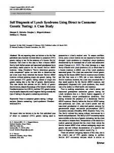
The N input elements xj are transformed into N output values x0j . A straightforward algorithm to compute the discrete Fourier transform would require O(N 2 ) steps. Cooley and Tukey [4] published the FFT algorithm, which completes the required calculation in O(N  2 log N ) steps. The algorithm is based on the property that an FFT of length N can be written as the sum of two FFTs of length N=2 [10]. The algorithm can be explained without going into mathematical detail. Figure 1 illustrates the data flow when an array of 8 elements is transformed.

x0

x1

x2

x3

x4

x5

x6

x7

HH  HH  HH  HH  4j    H H H w0H-H w0HH w0HHj- h? wH0HHj- h? level 0 using w j ?h j- h? h? h? h? h? XXXXX  XXXXX   X 9 w0 XXXX 9wX0 XXXXz- ?h z- ?h h? h? 2j XXXXX  XXXXX  level 1 using w 9wX2 XXXX 9wX2 XXXXz- ?h z- h? h? h? XXXXXX     XXX-Xz ?h 0 ?h 9 0 x4 w x00 XXXXXX     level 2 using w1j XXX-Xz h? 0 9 h? 1 x w 5 x01 XXXXXXX     XX-Xz ?h x0 9  h? 2 w 6 x02  X  XXXXXXX     ? X-Xz ?h x70 9  h w3 x03

Figure 1: The data flow in a fast Fourier transform The input hx0 : : : xN ?1 i is transformed to hx00 : : : x0N ?1 i in 2 log N (= 3) steps. Each step calculates an intermediate array from its input values, shown as levels 0, 1 and 2 in figure 1. On each level, the input array is fed in pairs into N=2 independent calculations, shown as cells in figure 1. The computation within each cell, called a butterfly because of its graphical appearance, is the following:

x0j x0k

= =

xj ? wj xk xj + wj xk

or as a function definition:

b y

n x y = (x + z; x ? z)

where

z = wn  y

In figure 1, a butterfly is shown as two circles connected by three arrows. What changes from level to level is the span of each butterfly (k = j + 2level ) and the positions where butterflies are applied. An extra complication for the FFT is the order of the input elements at level 0. Before entering the dataflow diagram the input elements must be permuted. In figure 1 this permutation is 0,4,2,6,1,5,3,7. This seemingly complex permutation is derived by reversing the bits in the binary representation of the index. For instance the third input element (index = 0112) in an 8-element FFT is x1102 = input 6 .

An important aspect of the calculations in figure 1 is the fact that reversing the direction of the dataflow does not influence the result. It is thus possible to perform the FFT from the bottom to the top. In that case the dataflow within a butterfly has to be upside down. Instead of permuting the input, the output then has to be reordered, according to the same bit reversal of indices. The two directions, top down and bottom up give rise to fundamentally different programs, a recursive one and an iterative one. In the literature only the iterative algorithm is generally shown [3], because loops are more efficient than recursive function calls in traditional imperative languages. In functional languages, however, we can consider both variants, because iteration and recursion are the same.

3 Two different implementations The invariance of the FFT to the direction of dataflow in figure 1 leads to two different versions of the algorithm. The recursive variant always traverses the input elements in strict sequential order, whereas the iterative version traverses the input elements in a more complicated order. The latter version seems wel suited for arrays, the former for lists.

3.1 An iterative implementation Considering the top down data flow in figure 1, we observe that the left inputs of all butterflies are connected in a regular way to the outputs on the next higher level. The regularity is the following: the left wing of a butterfly at level m is connected to xj at level m ? 1, when the binary representation of j has a zero in the m-th bit position. In figure 1 for example, the left inputs of the butterflies at level 1 are connected to x0 , x1 , x4 , x5 , because bit 1 is zero in 0,1,4 and 5. The implementation in figure 2 is based on the observed regularity. The first argument n of the iterative function ifft is used to compute the current level m and terminates the recursion when all levels have been handled. > > > > > > > > > > > > >

imain :: [complex] imain = ifft (inputsize div 2) (reorder inputsize input) ifft :: num -> [complex] -> [complex] ifft 0 xs = xs ifft n xs = ifft (n div 2) xs’ where m = log2 (inputsize div (n * 2)) xs’ = mkarray [mkpair j | j [num] bits = map (mod 2) . iterate (div 2)

Figure 2: An iterative implementation of the FFT in Miranda A list comprehension is used to express all butterfly applications on one level m. The function bits transforms an integer into its binary representation as a list of 0’s and 1’s. The mentioned regular connections of the left inputs xj of the butterflies are expressed in the program by the restriction (bits j) ! m = 0. The span of the butterflies at level m is 2m , so the index for the right inputs xk is k = j + 2ˆm .

The function mkarray takes a list of index pairs and corresponding value pairs to construct a new array. Array indexing is denoted in the same way as list subscription. The function imain of figure 2 can be tested on a Miranda system when a list version of mkarray is used. In the appendix a Miranda implementation of the bfly function and all auxiliary functions is given for reference. Our experiments were performed with an implementation of a lazy functional language that provides efficient arrays and O(1) array indexing, efficient bit manipulation functions etc. (see section Experiments). So in the experiments, we use the array and listarray functions as described in the introduction and bits is implemented with a few logical shift and mask operations.

3.2 A recursive divide and conquer implementation Next we consider the bottom up dataflow in figure 1. The data flows from level 2 up to level 0. In the first step the butterfly operation is performed on all input elements x0j at level 2. The resulting array can be split into two equal parts, a left part and a right part, each consisting of four elements (see figure 1, level 1). We observe that the rest of the calculations are two recursive repetitions of what has already been done on respectively the left part and the right part. Figure 3 shows an implementation following this line of thought. The first argument n of the recursive rfft is necessary to calculate the required root of unity. > > > > > > > > > > >

rmain :: [complex] rmain = reorder inputsize (rfft 0 input) rfft :: num -> [complex] -> [complex] rfft n [x] = [x] rfft n xs = rfft (n div 2) ls’ ++ rfft (n div 2 + inputsize div 4) rs’ where ls’ = map fst pairlist rs’ = map snd pairlist pairlist = map2 (bfly n) ls rs (ls,rs) = split (#xs div 2) xs

Figure 3: A recursive implementation of the FFT in Miranda The butterfly calculations can be arranged in such a way that the input is traversed in sequential order. On level 2 in figure 1, the span of the butterfly is exactly half of the input size. If the input is split in two equal parts, the left half ls always forms the left input of all butterflies at level 2 and the right half rs always the right input. In figure 3 the sequential traversal is performed by the function map2. This function applies the butterfly element wise to ls and rs. The resulting list is a list of pairs. The left elements of all these pairs are assembled into ls’ and the right elements into rs’. In contrast to the recursive implementation the iterative implementation selects input values in a non sequential order. The butterflies are applied at regular, but not always adjacent positions ((bits j) ! m = 0). There is no cheap way to split the input beforehand in two lists for the left and right inputs of the butterfly. Arrays have an advantage in this situation. However, it is not clear that this implementation with arrays, as a whole, will be faster than the recursive version with lists. Before discussing this issue we must first try to improve the efficiency of the basic variants.

4 The FFT variants In the previous section the principal aspects of two different FFT implementations were discussed. No attention has yet been paid to efficiency. This section describes the more efficient versions of the FFT, on which our measurements are based. In particular the possible advantage of using arrays is considered in each case. > rllfft :: num > rllfft n [x]= > rllfft n xs = > > > > >

-> [complex] -> [complex] [x] rllfft (n div 2) ls’ ++ rllfft (n div 2 + inputsize div 4) rs’ where ls’ = map2 add ls rs’’ rs’ = map2 sub ls rs’’ rs’’ = map (mul (unitroot n)) rs (ls,rs) = split (#xs div 2) xs

Figure 4: Unfolding the Butterfly gives the recursive, list in, list out version rllfft

4.1 Variants of the recursive implementation The efficiency of the basic recursive implementation in figure 3 can be improved substantially. The applications of map fst and map snd are only needed to unpack the pairs produced by the butterfly calculations. Unfolding the butterfly function allows direct computation of the intermediate arrays ls’ and rs’, which avoids the use of map fst and map snd altogether. This is illustrated in figure 4, where the functions add, sub and mul implement the operations +, ? and  on complex numbers and unitroot computes the power of the appropriate root of unity in the complex plane (see appendix). This version will be referred to as rllfft, for recursive, list in, list out FFT. Using arrays we can further improve the FFT version of figure 4. When the input values are stored in an array, the right hand part of the input can be accessed directly without having to split the input beforehand. The gain of avoiding the application of split should be compared against the extra work to construct arrays for ls’ and rs’. Our implementation uses the function tabulate to do this. As discussed in section 1 there is little overhead in this operation compared to list construction. Figure 5 shows the array version ralfft of figure 4, together with the required arithmetic functions over arrays. Another variant is obtained when the output values of the FFT are also stored in arrays. We expect no real advantage in doing this, because the output of the FFT is produced in sequential order. The results of recursive invocations are just appended. Appending arrays is not cheaper then appending lists, at least in terms of space consumption. Still we include the figures on this variant because it uses arrays for both input and output. This version will be referred to as raafft, for recursive, array in, array out.

4.2 Variants of the iterative implementation We did not use the iterative version as it is presented in figure 2. Unfolding the list comprehension yields a more efficient version. The restrictions on the indices j and k can be replaced by a simple calculation. What is obtained is similar to the version presented in [10]. This version is called iaafft for iterative, array in, array out. There is a possibility to improve the iterative version iaafft. It is rather expensive to construct the intermediate array on each level by the function mkarray, because first a list

> > > > > > > > > > > > > > > >

ralfft :: num -> [complex] -> [complex] ralfft n [x] = [x] ralfft n xs = ralfft (n div 2) ls’ ++ ralfft (n div 2 + inputsize div 4) rs’ where ls’ = tabulate (add ar xs rs’’) (1,n2) (1,n2) rs’ = tabulate (sub ar xs rs’’) rs’’ = tabulate (mul ar (unitroot n) xs n2) (1,n2) n2 = #xs div 2 add ar :: [complex] -> [complex] -> num -> complex sub ar :: [complex] -> [complex] -> num -> complex mul ar :: complex -> [complex] -> num -> num -> complex ) add ar xs rs’’ i = add (subscript xs i) (subscript rs’’ i sub ar xs rs’’ i = sub (subscript xs i) (subscript rs’’ i ) mul ar c xs n2 i = mul c (subscript xs (i+n2))

Figure 5: With arrays no split is needed for the recursive, array in, list out ralfft is constructed with indices and corresponding values. However, the use of mkarray can be avoided when the output values of each butterfly are not put directly into the right place, but merely assembled into a list. For the next iteration this means that the input values are in a different position. When the intermediate list is converted into an array, the fact that values are in a different place does not increase access time. However, the interconnection pattern of the FFT becomes more complicated and the savings by avoiding mkarray should be compared against more complex index calculations. The version thus obtained is called ialfft for iterative array in, list out. Considering the implementation of figure 2 one can expect that the calculation of the indices j, k and of the rotation unitroot (n*j) inside the butterfly will consume a lot of time, because they are repeated for each element (i.e. N  2log N times). This observation also holds for the more efficient unfolded version of figure 2 that we have used in the measurements. It is possible to compute the numbers j, k and unitroot (n*j) in advance for a given size of the input to the FFT. We have made two variants of the iterative FFT with different amounts of precomputation. The version with full precomputation requires O(N  2 log N ) storage. Only O(2 log N ) storage is required for the version with partial precomputation. Partial precomputation requires additional runtime to compute the remaining information during the FFT process. The version with a partial precalculation is called piaafft. That with full precalculation is called fiaafft. For the recursive variant precomputation is of no use because no indices are needed. The resulting precalculating iterative FFTs are both faster than the one without precalculation, but they can only be used with a fixed input size. In practice FFT computations are often repeated on input sets of the same size, so the precomputation can even be reused.

4.3 A synthetic variant The idea of precomputation can be extended further. The dataflow diagram of figure 1 can be turned into one large tree of function applications. The circles in the figure are the function applications and the arrows indicate how the applications are nested. The intermediate results do not need to be stored in data structures of any kind. All function applications are inputs to other function applications until the top level. This idea is illustrated in figure 6 for an FFT

on four input values. The function fft4 uses list pattern matching to name the four elements of the input list. Here the reordering could be implemented at no extra charge by changing [b00,b01,b02,b03] into [b00,b02,b01,b03], which is not the case for the non synthetic versions. The function fft4 can be improved in the same way as the other variants by unfolding the butterfly and subsidiary functions and allowing common subexpressions to be shared. > fft4 :: [complex] -> [complex] > fft4 [b00,b01,b02,b03] > = [b20,b21,b22,b23] > where > (b10,b11) = bfly 0 > (b12,b13) = bfly 0 > (b20,b22) = bfly 0 > (b21,b23) = bfly 1

b00 b02 b10 b11

b01 b03 b12 b13

Figure 6: Synthetic FFT in Miranda for an input with a fixed size (4) A precomputed tree of function applications is the fastest FFT that is possible in functional languages. All function applications are elementary computations.

5 Experiments The 8 different versions of the FFT have been presented as Miranda programs because of its widespread use. However, Miranda does not provide array primitives, so in this case it is not suitable for performance measurements. The programs were translated by hand into a functional language called intermediate [7], which is a simple, lazy, curried, higher order functional language that provides lists, arrays, complex numbers, double precision numbers and integer numbers as basic data structures. The language offers all the primitive functions required to efficiently operate on these data structures, including the bit manipulation functions needed by some of the FFT variants. The translation from Miranda to intermediate requires lambda lifting, the translation of pattern matching into conditionals and the translation of list comprehensions in function calls. Standard techniques for these translations are described in [9]. The intermediate version of the synthetic 4-point FFT thus obtained is shown in figure 7. The syntax is similar to that of Miranda, except that LET-expressions are used instead of where expressions. The pattern matching on the argument of fft4 is made explicit in the intermediate version by applications of head and tail. It has been assumed that the function will not be applied to lists with less than 4 elements. The calls to the bfly and subsidiary functions are unfolded, as in the transition from rfft to rllfft. This yields two common sub expressions, which are represented by the LET-expressions for w0 and w1. All variants of the FFT have been translated from Miranda to intermediate in the best possible way. This avoids an uneven bias in the performance comparison. The observed differences can thus be attributed entirely to the use of arrays. Intermediate forms the intermediate (hence the name) between the front end of a modern functional language, such as Haskell or Miranda, and our back end: the FAST compiler [7]. The back end compiles programs written in intermediate into equivalent C programs and also performs extensive analysis and code optimisation on the programs being compiled. The C programs are subsequently compiled by the C compiler and linked with the intermediate

fft4 i1 = LET LET LET LET LET

IN

b00=head i1 IN LET i2=tail i1 IN b02=head i2 IN LET i3=tail i2 IN b01=head i3 IN LET i4=tail i3 IN b03=head i4 IN b10=add b00 r00; b11=sub b00 r00; b12=add b02 r01; b13=sub b02 r01; b20=add b10 r10; b22=sub b10 r10; b21=add b11 r11; b23=sub b11 r11; w1 =complex 0.0 1.0; w0 =complex 1.0 0.0; b20:b21:b22:b23:NIL;

r00=mul r01=mul r10=mul r11=mul

b01 b03 b12 b13

w0; w0; w0; w1;

Figure 7: Synthetic 4-point FFT translated from Miranda to intermediate runtime library to form the executables. The effect of the optimisations on the performance of a benchmark of functional programs is studied in [6]. The fact that the FAST compiler ultimately produces a C program for each of the FFT variants opens up the possibility to compare the runtime of the variants with an original C version of the FFT. The FORTRAN version of the FFT as presented in [10, Pages 394-395] served as the basis for this C implementation. To improve the compatibility with the functional versions of the algorithm, instead of a double length array containing alternate real and imaginary parts of the complex numbers, a proper data type typedef struct { float re,im; } complex; is used. The input data may thus be declared as complex input[2048];. The runtime of the C version is about 0.5 sec for the 2048 point transform. This was measured on the same machine as that used for the functional versions to be discussed in the next section.

5.1 Metrics The FAST runtime system gathers simple run time statistics by counting cell claims and function calls. This does not significantly influence the execution time. The performance of an intermediate program can thus be measured in cpu seconds. This gives a useful, but rather crude performance measure. To identify program sections that are relatively often used and therefore perhaps a source of inefficiency, other measures are also needed. We use two sets of parameters for this purpose. The first set counts the number of calls to certain classes of functions. These are readily related to the program text and tell us something about the number of times sections of code are executed. The major classes are: user

a user defined function.

array

an array primitive.

complex

a complex operation, such as mul, add and sub.

other

any other function, such as head or cons.

total

all of the functions above as a total.

The second set of parameters counts the number of times space is claimed to store an object in the heap. These parameters are useful because in an implementation of a lazy functional language, a considerable fraction of the run time is spent on garbage collection [5]. Our FFT versions are too small to trigger the garbage collector, so it would appear that storage allocation is free. To quantify the cost of storage management we count the number of times we allocate:

CONS

a constructor cell.

ARRAY

a block of memory to hold pointers to all the array elements.

NUM

an integer, a double precision, or a complex number.

AP

a binary or vector application node.

TOTAL

all of the objects above as a total.

The measurements exclude any of the pre- or postprocessing that is necessary to fully implement the FFT transforms. The iterative variants require reordering before the actual transform, while the recursive variants need the reordering after the transform. Preprocessing further includes preparing the input data and computing the required roots of unity. Post processing also takes care of neatly printing the results. The sum of pre- and postprocessing involves the same amount of work for all variants of the FFT. Hence, it is not useful to account for pre- and postprocessing in the comparison of the variants. It would only offset the result by a constant factor, thereby obscuring the relative performance figures.

5.2 Statistics for the synthetic FFT The FAST compiler is a pilot version. It has some limitations, which make it impractical to compile a program with a single large function. The synthetic FFT that accepts 128 input points requires a where clause with 128  7=2 = 448 definitions, which is about the largest we can handle. However, because the number of function calls, cell claims etc. only depend on the size of the input, and not on the actual data values, we can scale up the results for smaller input data sets to arrive at exact statistics for a 2048 point transform. This is the size of the input data set that was used for the 7 non synthetic FFT implementations. Table 1 shows the formulae that express the dependence of the proposed metrics on the size of the input data set. These formulae were determined from the program text for synthetic FFT versions written to handle smaller input sets. For example, figure 7 shows that the functions mul, add and sub are each called n  2 log n=2 times, which for n = 4 amounts to 4 times. The total number of complex operations is thus 3  n  2 log n=2 = 1:5n  2 log n. A similar reasoning yields the parameters a, b and c in the general expression an  2 log n + bn + c for each of the parameters shown in table 1. parameter function user complex other total

=

an  2log a 1.5 1.5 0 3

+

bn b

2.5 0.5 3 6

+

c c

1 -1 -1 -1

parameter cell type CONS NUM AP TOTAL

=

an  2log a

0 9 1.5 10.5

+

bn b 2 1 2 5

+

c c

0 0 -1 -1

Table 1: Dependence of parameters on input data size n To estimate the execution time of the synthetic FFT for an input size of 2048 as used with the other versions is not so easy. Time measurements can not be extrapolated reliably because of systematic effects in a complex computer architecture. Instead, we use an estimate for the minimum amount of time that such a transform must take. The minimum is measured by using a small program constructed to claim as many cells as the 2048-point synthetic transform, which also calls the same number of functions. The execution time of this program is about 1 second, thus the synthetic 2048 point transform must take at least 1 second. This result appears as > 1 in table 2.

5.3 Results The top half of table 2 shows the function call statistics for each of the 8 FFT transforms. The bottom half of the table shows the cell claim statistics. As indicated before, these figures apply purely to the FFTs, without any pre- or postprocessing. The measurements exhibit a strong correlation (of 0.98 and more) between the metrics total, TOTAL and seconds. This means that either provides a good indication of the overall performance.

user array complex other total

Recursive versions rllfft raafft ralfft 216044 117756 101366 2049 96239 61435 33792 33792 33792 209901 53240 38908 461786 301027 235501

CONS ARRAY NUM AP TOTAL

Recursive versions rllfft raafft ralfft 130044 3072 23552 4 15351 8186 204799 259068 236542 148460 71668 61426 483307 349159 329706

Function calls Iterative versions iaafft ialfft piaafft 202779 319517 181277 56342 37912 47125 33792 33792 33792 191539 867379 120884 484452 1258600 383078

fiaafft 135203 45078 33792 67640 281713

Synthetic fft2048 38913 0 34816 6143 79872

fiaafft 45045 45078 214027 123915 428065

Synthetic fft2048 4096 0 204800 37887 246783

4.04

>1

Cell Claims

seconds

5.03

4.26

3.3

iaafft 45045 45078 281617 180224 551964 5.77

Iterative versions ialfft piaafft 45045 88054 24 45078 508945 223244 159746 143367 713760 499743 7.36

4.52

Table 2: Statistics for the 8 functional versions of the FFT

Discussion of the recursive variants The first data column of table 2 show performance statistics of the basic recursive version rllfft. Comparison with the third data column marked ralfft shows that using arrays for input in the recursive variant reduces execution time by about 34 %. This is caused by the application of split (see figure 3), which takes a considerable amount of time. As expected the use of arrays for the construction of output as in raafft is not advantageous. Constructing arrays and appending arrays is more expensive than the corresponding operations on lists. The recursive variant rllfft, which was described as a function operating purely on lists, still uses some array operations. This is due to the fact that the list output has to be converted into an array for the reorder during post processing. All versions use the same reorder algorithm based on array input. Discussion of the iterative variants The basic iterative version iaafft uses fewer CONS cells than the basic recursive version rllfft. Instead, iaafft uses more ARRAY cells than rllfft. This agrees with our expectations. The overall performance of iaafft, however, is worse than rllfft. This is due to the complicated index calculations (j and k in figure 2) and is reflected in the larger number of NUM cells (281617 versus 204799) and other function calls (551964 versus 483307).

Version ialfft avoids the construction of intermediate arrays, which is reflected in the reduction of the number of ARRAY cells from 45078 to 24. The overall performance of ialfft is worse than that of iaafft, because the index calculations become more complex and an extra reorder is needed. This extra reorder is not included in the precomputation but explicitly accounted for in the performance figures presented in table 2, because ialfft is the only version that requires two reorders. The decreasing numbers for NUM and other in columns piaafft and fiaafft show that precomputation of index values pays off as expected. The performance of the best iterative version fiaafft is, however, still worse than the best recursive version ralfft. The number of ARRAY cells used by piaafft and fiaafft is exactly the same as for the basic iterative variant ialfft. This is expected because the precomputed indices are stored in lists and the index computations themselves do not use arrays. The partially precalculating version piaafft uses more CONS cells than the other iterative versions because it needs lists to calculate part of the indices during the FFT process. Discussion of the synthetic variant The best performance is achieved with the synthetic fft2048, the scaled up version of that shown in figure 6. It uses no ARRAY cells and only 4096 CONS cells to build the output list. Because the output of the synthetic FFT is a list, all applications of bfly appear in a lazy context. Therefore suspensions must be built, which explains why the synthetic variant claims AP nodes. The same holds for all the other variants, so that the same number of AP nodes claimed by each variant is due to the output being a lazy list or a lazy array. This constitutes an even bias in the comparisons. General remarks about all variants The number of operations on complex numbers does not depend on the variant of the FFT that is used. In the table this is reflected by the number 37912 in the row complex, which is exactly 1:5N  2 log N , with N = 2048. Only the synthetic FFT uses slightly more (3%) computations because it does not use the precomputed roots of unity but calculates them during the FFT process. We found that the ranking of the results did not depend on the size of the input. So the best version remains the best for all inputs that we tried: 128, 256, 512, 1024 and 2048.

6 Conclusions We have implemented eight versions of the FFT in a lazy functional language. There are three main types of the FFT:

  

The synthetic version represents the basic idea, where the entire pattern of calculations has been spelled out explicitly. This version carries no overhead for the management of data and was indeed found to be the fastest. The divide and conquer version works by recursively dividing the input data set into halves, performing the necessary calculations and then merging the results. The nature of the FFT makes it necessary to reorder intermediate results, because these are not produced in the order in which they are required. The classic iterative butterfly version of the FFT steps through the data, by selecting the inputs for each butterfly using a non trivial index calculation.

A comparison between the iterative and the recursive version of the FFT is not common in the literature. Our derivation of both algorithms from the same diagram, by reversing the data flow, provides a better understanding of the origin of both variants. The purely iterative version of the FFT does not achieve the best possible performance, even when the complicated index calculations are performed beforehand, and thus not accounted for. The overhead of array construction is too large. The same effect is shown by the recursive version raafft, where arrays are constructed rather than just subscripted as is the case in the best non synthetic variant ralfft. The basic recursive implementation using lists performs only slightly better than the basic iterative version. This is because it is expensive to split the input when it is represented as a list. The best performance is achieved when arrays are used for subscripting input data in the recursive variant. No arrays need to be constructed and no split of the input is required. Our measurements show that algorithms as published in literature for imperative languages cannot always be translated directly into a functional language, because efficiency considerations are of a different nature. We also conclude that an efficient implementation of arrays contributes significantly to the performance of functional languages in certain areas. However, a clear distinction should be made between array construction and array subscription. In the FFT example we could not gain efficiency by using array construction, other than for storing precomputed data like the input. The best performance is achieved with the synthetic FFT. The performance of the best non synthetic version (ralfft) is still a factor of at most three worse than that of the synthetic FFT. The performance of the synthetic FFT is about a factor of two worse than that of a standard FFT implementation made directly in C. This shows that still many things can be improved by a further development of compiler technology for functional languages.

Acknowledgements We thank Marcel Beemster and Henk Muller for their comments on a draft version of the paper. The two referees provided useful suggestions for improving the paper. The FAST compiler represents joint work with Hugh Glaser and John Wild, which is supported by the Science and Engineering Research Council, UK, under grant No. GR/F 35081, FAST: Functional programming for ArrayS of Transputers.

References [1] H. P. Barendregt and M. van Leeuwen. Functional programming and the language Tale. In J. W. de Bakker, W.-P. de Roever, and G. Rozenberg, editors, Current trends in concurrency: overviews and tutorials, LNCS 224, pages 122–208, Noordwijkerhout, The Netherlands, Jun 1985. Springer-Verlag, Berlin. [2] A. Bloss. Update analysis and the efficient implementation of functional aggregates. In J. Stoy, editor, 4th Functional programming languages and computer architecture, pages 26–38, London, England, Sep 1989. ACM, New York. [3] K. M. Chandy and J. Misra. Parallel program design: A foundation. Addison Wesley, Reading, Massachusetts, 1988. [4] J. W. Cooley and J. W. Tukey. An algorithm for the machine calculation of complex Fourier series. Mathematics of computation, 19(90):297–301, Apr 1965.

[5] P. H. Hartel. Performance of lazy combinator graph reduction. Software—practice and experience, 21(3):299–329, Mar 1991. [6] P. H. Hartel, H. W. Glaser, and J. M. Wild. On the benefits of different analyses in the compilation of functional languages. In H. W. Glaser and P. H. Hartel, editors, 3rd Implementation of functional languages on parallel architectures, pages 123–145, Southampton, England, Jun 1991. CSTR 91-07, Dept. of Electr. and Comp. Sci, Univ. of Southampton, England. [7] P. H. Hartel, H. W. Glaser, and J. M. Wild. Compilation of functional languages using flow graph analysis. Software—practice and experience, 24(2):127–173, Feb 1994. [8] P. Hudak, S. L. Peyton Jones, and P. L. Wadler (editors). Report on the programming language Haskell – a non-strict purely functional language, version 1.2. ACM SIGPLAN notices, 27(5):R1–R162, May 1992. [9] S. L. Peyton Jones. The implementation of functional programming languages. Prentice Hall, Englewood Cliffs, New Jersey, 1987. [10] W. H. Press, B. P. Flannery, S. A. Tekolsky, and W. T. Vetterling. Numerical recipes – The art of scientific computing. Cambridge Univ. Press, Cambridge, England, 1986. [11] D. A. Turner. Miranda system manual. Research Software Ltd, 23 St Augustines Road, Canterbury, Kent CT1 1XP, England, Apr 1990.

Appendix – Butterfly and auxiliary functions in Miranda Together with the functions shown in the appendix, the FFT versions described in the paper form a complete program. Because of its widespread use, we present programs in Miranda instead of intermediate, the language we use to perform our experiments in. All array functions discussed in the introduction, which are shown here as list processing functions in Miranda, are available as efficient primitives in intermediate. > > > > > > > > > > > > > > >

listarray :: [*] -> [*] listarray a = a tabulate :: (num -> *) -> (num,num) -> [*] tabulate f (l,u) = [f i | i num -> * subscript ar i = ar!(i-1) update (x:xs) = update (x:xs) =

0 y y : xs (i+1) y x : update xs i y

The select function searches the list of tuple-tuples produced by the list comprehension in ifft of figure 2 to find the complex number vj or vk with index m. > select :: * -> [((*,*),(**,**))] -> ** > select m (((j,k),(vj,vk)):rest)

> = vj , if j = m > = vk , if k = m > = select m rest , otherwise > > mkarray :: [((num,num),(*,*))] -> [*] > mkarray xs = listarray [select j xs | j log2 :: num -> num > log2 x = entier (log x / log 2)

Butterfly function > > > > > > > > >

bfly :: num -> complex -> complex -> (complex,complex) bfly n x y = (add x z, sub x z) where z = mul (unitroot n) y unitroot :: num -> complex unitroot n = C (cos phi) (sin phi) where phi = 2 * pi * n / inputsize

Complex numbers and arithmetic > > > > > > > >

complex ::= C num add :: complex -> sub :: complex -> mul :: complex ->

num complex -> complex complex -> complex complex -> complex

add (C x y) (C u v) = C (x+u) (y+v) sub (C x y) (C u v) = C (x-u) (y-v) mul (C x y) (C u v) = C (x*u - y*v) (x*v + y*u)

Sample input data > > > > > > > > > > >

inputsize :: num inputsize = #input indices :: [num] indices = [0 .. (#input - 1)] input :: [complex] input = [C 1 C 1 C 1 C (-1)

0,C 1 0,C 1 0,C 1 0, 0,C 1 0,C 1 0,C 1 0, 0,C (-1) 0,C (-1) 0,C (-1) 0, 0,C (-1) 0,C (-1) 0,C (-1) 0]

Reordering > > > > > >

split :: num -> [*] -> ([*],[*]) split n xs = (take n xs, drop n xs) join :: num -> [*] -> [*] -> [*] join n [] []= [] join n x y = firstx ++ firsty ++ join n restx resty

> where > (firstx,restx) = split n x > (firsty,resty) = split n y > > reorder :: num -> [*] -> [*] > reorder 1 y = y > reorder n y = reorder (n div 2) (join m left right) > where > (left, right) = split (inputsize div 2) y > m = inputsize div n