Artificial Bee Colony for Constraint Satisfaction Problems

SCIS-ISIS 2012, Kobe, Japan, November 20-24, 2012

Artificial Bee Colony for Constraint Satisfaction Problems Yuko Aratsu, Kazunori Mizuno, Hitoshi Sasaki Department of Computer Science Takushoku University Hachioji, Tokyo 193-0985, Japan Email: [email protected], [email protected]

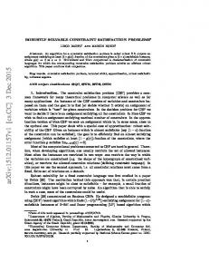
X = {x1 , x2 , x3 , x4 } D = {a, b, c} (= D1 = · · · = D4 ) C = {c12 , c23 , c14 } c12 = {(a b), (b c)} c23 = {(c b), (b a), (b b)} c14 = {(a c)} Solutions: (x1 x2 x3 x4 ) = {(a b a c), (a b b c)}

Abstract—In this paper, we propose the artificial bee colony algorithm for solving large-scale and hard constraint satisfaction problems (CSPs). Our algorithm is based on the DisABC algorithm which is proposed to solve binary optimization. We describe the detailed algorithm and brief experiments, demonstrating that our algorithm can be effective to solve CSPs.

Figure 1.

Keywords-constraint satisfaction; search; meta heuristics; artificial bee colony;

An example instance of binary CSPs.

Binary CSP instances for using the experiments can be generated randomly. A class of randomly generated instances is characterized by 4 components, ⟨n, m, p1 , p2 ⟩ where n is the number of variables, m is the domain size, or the number of values, p1 is the probability of adding a constraint between two different variables, and p2 is the probability of ruling out a pair of values between two constrained variables.

I. I NTRODUCTION To solve large-scale and hard constraint satisfaction problems (CSPs) that are NP-complete, metaheuristics for stochastic search approaches has been recently made remarkable progress[1]. Artificial bee colony (ABC) [2], based on the intelligent foraging behaviour of honeybee swarm, is one of typical meta-heuristics. Although it is expected that the ABC algorithm can be effective for many search problems, the ABC algorithm can not be directly applied to CSPs that are one of typical combinatorial search problems because the original ABC algorithm[2] is only able to optimize continuous optimization problems. In this paper, we propose an ABC algorithm for solving CSPs, extending DisABC, proposed by [3], which can be applied to binary optimization. II. P ROBLEM DEFINITION AND ABC

Seiichi Nishihara Department of Computer Science University of Tsukuba Tsukuba, Ibaraki 305-8573, Japan Email: [email protected]

B. ABC Algorithm The ABC algorithm is a population-based meta heuristics inspired by the intelligent foraging behavior of honeybee swarm[2]. The foraging bees are classfied into three categories of employed, onlookers, and scouts. Employed bees determine a food source within the neighbourhood of the food source in their memory. They share their information with onlookers within the hive and then the onlookers select one of the food sources. Onlookers select a food source within the neighbourhood of the food sources chosen by themselves. An employed bee of which the source has been abandoned becomes a scout and starts to search a new food source randomly. In the ABC algorithm, the position of a food source is a possible solution of the optimization problem and nectar amount of a food source corresponds to the fitness of an associated solution.

ALGORITHMS

A. Constraint Satisfaction Problem Let us briefly give some definition and terminology about CSPs. A CSP is defined as a triple (X, D, C) such that • X = {x1 , . . . , xn } is a finite set of variables, • D is a function which maps every variable xi ∈ X to its domain Di , i.e., the finite set of values that should be assigned to xi , and • C is a set of constraints, each of which is a relation between some variables which restricts the set of values that can be assigned simultaneouly to these variables. In this paper, let D1 = · · · = Dn = D and |D| = m. We also employ binary CSPs which have only binary constraints, i.e., every constraint involves exactly two variables. Fig. 1 gives an example of binary CSP instances.

C. DisABC Algorithm The ABC algorithm has been designed for optimization in continuous space and cannot work with vectors with discrete values. In contrast, the DisABC algorithm has been proposed to solve binary optimization[3]. In the DisABC algorithm, to measure distance between food sources, the ”−” operator used in the original ABC algorithm is

2283


begin Initialization; For t = 1 to M axCycle do EmployedBeesPhase(); OnlookeredBeesPhase(); If rand < Gp then GSAT(X t ); End if ScoutBeesPhase(); Memorize the best solution achieved so far; End for end

substituted with a dissimilarity measure of binary vectors by employing the Jaccard coefficient of similarity[3]. Letting Xi = (xi1 , xi2 , · · · , xid , · · · , xiD ) and Xj = (xj1 , xj2 , · · · , xjd , · · · , xjD ) where xid and xid can take only 0 or 1 values, Dissimilarity (Xi , Xj ) is defines as Dissimilarity (Xi , Xj ) = 1 − Simmilarity (Xi , Xj ) , where Simmilarity (Xi , Xj ) = M11 = M10 M01 M00

∑D

d=1 I(xid ∑D = d=1 I(xid ∑D = d=1 I(xid ∑D = d=1 I(xid

M11 , M11 + M10 + M01

procedure EmployedBeesPhase() For i = 1 to N s do Generate a new assignment Vit from Xit (and based on Xkt (k ̸= i)) via NBSG proposed by [3]; Evaluate the new solution; If Conf (Vit ) < Conf (Xit ) then Xit ← Vit ; triali ← 0; Else Remember Xit ; triali ← triali + 1; End if End for end procedure

= xjd = 1), = 1, xjd = 0), = 0, xjd = 1), = xjd = 0).

III. T HE P ROPOSED A RTIFICIAL B EE C OLONY A LGORITHM A. Basic Strategies

procedure OnlookerBeesPhase() For i = 1 to N s do Calculate the probability proportional to the quality of food sources pi ; Produce a new assignment Vit from Xit (and based on Xkt (k ̸= i)) selected depending on pi via NBSG proposed by [3]; Evaluate the new solution; If Conf (Vit ) < Conf (Xit ) then Xit ← Vit ; triali ← 0; Else Xit+1 ← Xit ; triali ← triali + 1; End if End for end procedure

In this paper, we propose an ABC algorithm for solving CSPs, summarized as follows: i) The proposed algorithm is based on the DisABC algorithm which can solve binary optimization problems. ii) CSP instances to be applied to the our algorithm are encoded or reexpressed to a binary optimization form. iii) To supplement local search abilities of the ABC, GSAT proposed by Selman[4] is combined with our algorithm. Thus, our method can efficiently solve CSPs, although each CSP instance is needed to be reexpressed. B. The Algorithm Fig. 2 gives the proposed algorithm, in which DisABC is extended to solve binary CSPs. To apply binary CSP to our algorithm, CSP instances need to be reexpressed. Fig. 3 gives the procedure to reexpress CSP instances. For example, when the CSP instance denoted in Fig. 1 is applied to this procedure, The binary version is output as shown in Fig. 4. In Fig. 2, the ith food source, Xit (i = 1, · · · , N s), at the cycle t, which corresponds to the assignment of values to variables is first generated at ”Initialization”. Then, the main three processes, EmployedBeesPhase, OnlookerBeesPhase, and ScoutBeesPhase, are repeated until a solution with no coustraint violations, i.e., Conf (X) = 0, is found or t reaches M axCycle. Conf (X) is the number of constraint violations of X. GSAT, which can perform a greedy local search, is hybridized with our algorithm and is employed after the onlooker phase. Gp controls the rate of recalling the GSAT module in our algorithm.

procedure ScoutBeesPhase() If max {triali } ≥ limit then Replace the abandoned assignment with a new random assignment; End if end procedure Figure 2.

The proposed algorithm for solving CSPs.

IV. E XPERIMENTS A. Experimental Settings To evaluate the efficiency of the proposed methods, we attempt to briefly conduct the experiments. We employ binary CSP instances for the case of ⟨30, 4, 0.14, p2 ⟩. For 14 cases of p2 = 0.40, 0.42, 0.44, 0.46, 0.48, 0.50,

2284


begin Generate n × m variables; For i = 1 to n do For j = (i + 1) to n do If cij ∈ C then For k = 0 to (m − 1) do If k == (ci −′ a′ ) then ci(′ a′ +k) ← 1; Else ci(′ a′ +k) ← 0; End if If k == (cj −′ a′ ) then cj(′ a′ +k) ← 1; Else cj(′ a′ +k) ← 0; End if End for End if End for End for end Figure 3.

㪦㫌㫉㩷㪸㫇㫇㫉㫆㪸㪺㪿

parcentage of solved

0.9

0.7 0.6 0.5 0.4 0.3

0.1

0.6 4 0.6 6

0.6 0 0.6 2

0.5 6 0.5 8

0.5 2 0.5 4

0.4 8 0.5 0

0.4 4 0.4 6

0.4 0 0.4 2

0

P2

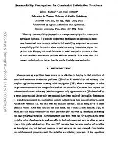
Figure 5.

Experimental result on the percentage of success.

The procedure to reexpress CSPs.

We evaluate the percentage of solved CSP instances, that is, the proportion of the number of instances for which the method can find a solution to all instances to be tried to search and average cycles required for solving. The method is implemented in language Java on a PC with 3.07GHz of Intel Core i7 880 and 4GBytes of RAMs. B. Experimental Results and Discussion Figs. 5, 6, and 7 give the results. Fig. 5 shows the percentage of solved CSP instances. Figs. 6 and 5 show the average of total cycles in our approach and the average of total flips in GSAT, respectively. When p2 = 0.50, around which very hard instances are concentrated, lowest percentage of success appears compared to other regions in our approach as shown in Fig. 5. A lot of cycles is also required in this region as well in Fig. 6. Although our algorithm can entirely solve generated instances with high probability, it should be important to conduct more experiments for much largerscale instances. On the otherhand, the performance of GSAT is not so good because GSAT can hardly solve instances in over-constrained regions whose instances seem not to be necessarily extremely hard, suggesting to us that it may be necessary to conduct experiments using other parameter sets.

An example instance of the reexpressed binary CSPs.

0.52, 0.54, 0.56, 0.58, 0.60, 0.62, 0.64 and 0.66, we randomly generate 100 instances per case, i.e., a total of 1400 generated instances, whose search space size is 430 (≃ 1018 ). However, the search space size of reexpressed ones is 2120 (≃ 1036 ). These instances are located around phase transition[5] regions derived by the following equation[6]: κ=

0.8

0.2

X = {(x1a , x1b , x1c ), (x2a , x2b , x2c ), (x3a , x3b , x3c ), (x4a , x4b , x4c )} D = {0, 1} (= D1a = · · · = D4d ) C = {c1∗2∗ , c2∗3∗ , c1∗4∗ } (*: a, b, or c) c1∗2∗ = {(1 0 0 0 1 0), (0 1 0 0 0 1)} c2∗3∗ = {(0 0 1 0 1 0), (0 1 0 1 0 0), (0 1 0 0 1 0)} c1∗4∗ = {(1 0 0 0 0 1)} Solutions: (x1∗ x2∗ x3∗ x4∗ ) = {(1 0 0 0 1 0 1 0 0 0 0 1), (1 0 0 0 1 0 0 1 0 0 0 1)} Figure 4.

GSAT

1

n−1 1 p1 logm ( ). 2 1 − p2

(1)

In particular, κ = 1.015(≃ 1) in the case of p2 = 0.50, correspoding to critically constrained regions. Let us clarify the parameter settings of the methods. The number, N s, of food sources is set to 50, ’M axCycle’ denoted in Fig. 2 is set to 10,000, and the number, limit, of trials for releasing a food source is set to n × m. As for parameters on GSAT in our algorithm, Gp and M AXF LIP S are set to 0.01 and 30, respectively. We also briefly conduct experiments on naive GSAT, in which parameters, M AX-T RIES and M AX-F LIP S in [4] are set to 5,000 and 100, respectively.

V. C ONCLUSION We have described a new approach to deal with CSPs using the ABC algorithm in this paper. In our method, CSP instances are converted to apply instances to the DisABC algorithm. We conduct brief experiments, demonstrating that our algorithm can be effective to solve CSP instances. Our most important future works should consist in immediately conducting more experiments and comparing with other meta-heuristics and swarm intelligence approaches such as particle swarm optimization[7].

2285


All

[5] Hogg, T., Huberman, B. A., Williams, C. P.: Phase transition and search problem, Artificial Intelligence, Vol. 81, pp. 1-16 (1996).

Solved only

4500

average of total cycles

4000

[6] Clark, D. A., Frank, J., Gent, I. P., MacIntyre, E., Tomov, N., Walsh, T.: Local Search and the Number of Solutions, Proc. CP’96, pp. 119-133 (1996).

3500 3000 2500

[7] L. Schoofs, B. Naudts: ”Swarm intelligence on the binary constraint satisfaction problem”, Proceedings of the IEEE Congress on Evolutionary Computation (CEC 2002), pp.1444-1449.

2000 1500 1000 500

0.4 0 0.4 2 0.4 4 0.4 6 0.4 8 0.5 0 0.5 2 0.5 4 0.5 6 0.5 8 0.6 0 0.6 2 0.6 4 0.6 6

0

P2

Figure 6. Experimental result on average of total cycles in our approach.

All

Solved only

500000 450000

average of total flips

400000 350000 300000 250000 200000 150000 100000 50000

0.4 0 0.4 2 0.4 4 0.4 6 0.4 8 0.5 0 0.5 2 0.5 4 0.5 6 0.5 8 0.6 0 0.6 2 0.6 4 0.6 6

0

P2

Figure 7.

Experimental result on average of total flipss in GSAT.

R EFERENCES [1] Mizuno,K.,Nishihara.S,et.al.: ”Population migration: a meta-heristics for stochastic approaches to constraint satisfaction problems”, Informatica, Vol.25, No.3, pp.421-429(2001). [2] D. Karaboga, B. Basturk: ”On the performance of artificial bee colony (ABC) algorithm”, Applied Soft Computing 8 (2008) pp.687-697. [3] Mina Husseinzadeh Kashan, Nasim Nahavandi, Ali Husseinzadeh Kashan: ”DisABC: A new artificial bee colony algorithm for binary optimization”, Applied Soft Computing 12 (2012), pp.342-352. [4] Selman, B., Levesque, H., and Mitchell, D.: A New Method for Solving Hard Satisfiability Problems, Proceedings of AAAI92, pp. 440-446 (1992).

2286