Artificial Network for Predicting Water Uptake under Shallow Saline ...

Journal of Scientific Research & Reports 7(5): 359-372, 2015; Article no.JSRR.2015.217 ISSN: 2320-0227

SCIENCEDOMAIN international www.sciencedomain.org

Artificial Network for Predicting Water Uptake under Shallow Saline Ground Water Conditions Houshang Ghamarnia1* and Zahra Jalili1 1

Department of Water Resources Engineering, Compass of Agriculture and Natural Resources, Razi University, P.O.Box: 1158, Post Code: 6715685438, Kermanshah, Iran. Authors’ contributions

This work was carried out in collaboration between both authors. Author HG designed the study, wrote the protocol, and wrote the first draft of the manuscript. Author ZJ managed the literature searches, analyses of the study performed the spectroscopy analysis and author HG managed the experimental process and author ZJ identified the species of plant. Both authors read and approved the final manuscript. Article Information DOI: 10.9734/JSRR/2015/17870 Editor(s): (1) Leszek Labedzki, Institute of Technology and Life Sciences, Kujawsko-Pomorski Research Centre, Poland. Reviewers: (1) Andy Anderson Bery, School of Physics, Universiti Sains Malaysia, Malaysia. (2) Abdel Razik Ahmed Zidan, Irrigation & Hydraulics Department, Mansoura University, Egypt. Complete Peer review History: http://www.sciencedomain.org/review-history.php?iid=1129&id=22&aid=9391

th

Original Research Article

Received 28 March 2015 Accepted 5th May 2015 th Published 25 May 2015

ABSTRACT Lysimetric experiments were conducted in order to determine the groundwater contributions by Black cumin. The plants were grown in 27 columns, each with a diameter of 0.40 m and packed with Silty clay soil. The factorial experiments were carried out using three replicates with randomized complete block designs and different treatment combinations. Nine treatments were applied during each experiment by maintaining groundwater with an EC of 1, 2 and 4 dS/m at three different water table depths (0.6, 0.8 and 1.1m). The groundwater contributions and plant root depths were measured by taking daily readings of water levels in Mariotte tubes and minirhizotron respectively. The four input neurons were total water use evapotranspiration (ETo), plant root depth (Zr), groundwater salinity (GS) and groundwater depth (Z). The output neuron gives maximum water uptake rate (Smax). The results showed that for different treatments, the best neural network was determined to be Multilayer Perceptron network (MLP) and the artificial neural network was very successful in terms of the prediction of a target dependent on a number of variables. This study indicates that the ANN-MLP model can be used successfully to determine groundwater observation by plant roots. Sensitivity analysis was undertaken which confirmed that variations in _____________________________________________________________________________________________________ *Corresponding author: Email: [email protected], [email protected];

Ghamarnia and Jalili; JSRR, 7(5): 359-372, 2015; Article no.JSRR.2015.217

tide elevation are the most important factors in simulation of groundwater estimation in a semi-arid region. The results of this study showed that the estimation of plants groundwater contribution by ANN-MLP model is very useful for a quick decision on irrigation management to save a high volume of good surface water quality. Keywords: Artificial neural networks; black cumin; salinity; groundwater observation; lysimeter; minirhizotron.

1. INTRODUCTION Iran is a country with an arid and semi-arid climate having an average rainfall of 252 mm. The scarcity of fresh water resources is the main obstacle on the agricultural and industrial development of the country. Almost 15.2% of the total area of the country (25 million hectares) are saline lands having been left untouched as a result of high salinity and alkalinity [1]. According to the United Nations Environment Program, by 2025, Iran will be one of 100 countries in the world with low renewable fresh water per capita while the value of available water resources per 3 capita will reach to approximately 816 m as the population grows to 120 million, which is almost 20% less than the amount of water needed per 3 capita (1000 m ). Iran will be one of the countries dealing with water scarcity problem in the near future. Therefore, in order to mitigate the adverse impacts of such severe shortage of the available water resources and also to meet the growing demands for food, the use of non-conventional water resources such as saline, brackish and treated sewerage and reused water should be given a greater attention [2]. The water quantities taken by different crops that use shallow groundwater of varying salinities during the past 50 years have been reviewed [3]. They reported that most of the studies in literature had been conducted with non-saline groundwater while only a small number of studies had been performed under varying saline shallow groundwater conditions. Also, the variations in different parameters including crops, soil, water table depths, water table quality, climate and different irrigation scheduling makes it difficult to generalize the results of groundwater contribution by different plants [3]. Few researches have been conducted on the adoption of groundwater use by plants, especially in semi-arid regions of different provinces including Kermanshah, Lorestan, Ilam and Kurdistan in the west and northwest Iran, where the available shallow groundwater with

different qualities can be used as a sub-irrigation scheme for different strategic crops or medicinal plants. Such schemes have been devised by the support of the state-run agricultural organizations for oil and medicine productions in recent years. The same schemes can be proposed in order to reduce the irrigation water requirements and maintain groundwater table at suitable depths during the growing season in semi-arid regions aforesaid where available surface water resources are scarce [2]. On the other hand, the ANNs are proven to be effective in modeling virtually any nonlinear function to an arbitrary degree of accuracy [4]. Artificial Neural Networks are now being increasingly used in the prediction and forecasting of variables involved in water resources [5-9]. A feed-forward neural network coupled developed with GA (Genetic Algorithm) to simulate the rainfall field. The technique implemented to forecast rainfall for a number of times using hyetograph of recording rain gauges. The results showed that when FFN (Feed Forward Neural network) coupled with GA (Genetic Algorithm), the model performed better compared to similar work of using ANN (Artificial Neural Network) alone [10]. A few applications of the ANN approach in groundwater related problems can be found in the literature [11,12]. Groundwater levels have been forecasted in an individual well by monitoring continuously over a period of time using ANN [13]. In another study a developed ANN model was used to forecast groundwater levels in an urban coastal aquifer [14]. The performance of the artificial neural network (ANN) model, i.e. standard feed-forward neural network trained with Levenberg–Marquardt algorithm, was examined for forecasting groundwater level at Maheshwaram watershed, Hyderabad, India. The model provided the best fit and the predicted trend followed the observed data closely (RMSE = 4.50 and R2 = 0.93). Thus, for precise and accurate groundwater level

360

Ghamarnia and Jalili; JSRR, 7(5): 359-372, 2015; Article no.JSRR.2015.217

forecasting, ANN appears to be a promising tool [15]. Additionally, a thorough review of literature by the authors have revealed that no researches have yet been done to determine the percentage of groundwater contributions under different salinity and groundwater depths by plants. The main objectives of the present study is to estimate the soil water fluxes and the contribution of groundwater to the overall water requirements of Black cumin (EC 1, 2 and 4 dS/m) at water table depths of 0.6, 0.80 and 1.10 m and a comparison to Shallow saline groundwater estimation by Artificial Neural Networks Model.

2. MATERIALS AND METHODS 2.1 Experimental Site The experiments were performed in the Irrigation and Water Resources Engineering Research Lysimetric Station No. 1 (47°9' E and 34°21' N at an elevation of 1,319 m), part of the Compass of Agriculture and Natural Resources, Razi University of Kermanshah, Western Iran. The experiments were conducted during 2 years from year 2011 to 2012 from the month of March to the month of July inclusive [16].

2.2 Climate, Irrigation Water and Soil Characteristics The region has a semi-arid climate with no rainfalls during summer. All daily meteorological and cumulative evaporation data from class A

pan were obtained from the regional meteorological station 100 m off the research station. Table (1) shows the average monthly meteorological data during both years of the study. The study was performed using 27 lysimeters installed at the lysimetric station. The factorial experiments were carried out with three replicates based on a randomized complete block design. Nine treatments were applied in each experiment using groundwater with EC 1, 2 and 4 dS/m to maintain groundwater depths of 0.60, 0.80 and 1.10 m. The lysimeters were initially saturated from bottom for each treatment with water quality of (1, 2 and 4 dS/m) up to depths of 0.60, 0.80 and 1.10 m for 2 weeks. Then, the profile storage contribution was measured for each treatment separately using gravimetric method. The saline water with EC of 1, 2 and 4 dS/m was produced by dissolving NaCl and CaCl2 (1:1 by mass). The 1.20 m high lysimeters were made of 0.40 m diameter polyethylene (PE) material pipes with a sealed bottom of polyethylene and fixed by special electrical equipment to prevent any possible water leaching. A 5-cm layer of gravel and a 5cm layer of sand were placed at the bottom of each lysimeter to promote unrestricted exchange with the groundwater supply. A Silty clay soil consisting of 54, 42.3 and 3.7% clay, silt and sand, respectively, was used in all the lysimeters [16]. The chemical components of the surface irrigation water, with the chemical and physical properties of the soil used in this study together are given in Tables (2) and (3).

Table 1. Climate data during growing period Year

Month

2011

March April May June July March April May June July

2012

Mean temperature (°c) 11 12.4 16.5 23.4 28 10 12.1 18.4 24 26.5

Mean relative humidity (%) 43 51 62 30 18 45 55 40 24 20

Mean wind speed (m/s) 10.7 12.2 10.2 14 21 11 14 24 20 15.4

Mean monthly sunshine (hr) 10.3 6.2 5.8 10.1 10.7 9.5 6.9 8.3 9.7 10.2

Total precipitation (mm) 0 46.9 119.7 0 0 0 45.7 17.9 0 0

Table 2. Chemical properties of surface irrigation water [17] Cations (Meq/l) 9.3

Ca2+ (Meq/l) 5.05

Na+ (Meq/l) 1.15

Mg++ (Meq/l) 3.1

Anions (Meq/l) 9.3

SO2(Meq/l) 1.25

361

CL HCO3- CO32(Meq/l) (Meq/l) (Meq/l) 1.9 6.15 0

PH 7.1

TDS (Meq/l) 390

EC (dS/m) 0.5

Ghamarnia and Jalili; JSRR, 7(5): 359-372, 2015; Article no.JSRR.2015.217

Table 3. Physical and chemical properties of soil [17] Soil texture Silt clay

Clay (%) 54

Silt (%) 42.3

Sand (%) 3.7

EC (dS/m) 0.6

θ(fc) (%) 17.2

The Silty clay soil used in the study was sieved using a conventional 2-mm mesh, and all the lysimeters were filled with air dried soil. The lysimeters were filled in 10-cm layers each soil layer was compacted manually to reach a bulk density of 1.30 g/cm3 (field soil bulk density) [18]. Soil field moisture characteristic curves (data not shown) were constructed [19]. In the experiments, Black cumin was used as crop material. Black cumin seeds were planted on March 27th, 2011 and March 27th, 2012 at depths 2 of 2 cm with a seeding density of 40 per m . The water table levels were controlled in all lysimeters at 0.60, 0.80 or 1.10 m below the soil surface. Before creating different groundwater depths, the seeds received 10 mm of surface water (EC 0.5 dS/m) in all treatments with supplementary irrigation during the experimental period. Further irrigation treatments were applied when 4 or 5 leaves were observed on each plant and at the 38th day after planting. The total water applied for each treatment consisted of surface irrigation water, groundwater contributions (GWC), rainfalls and profile storage contributions. The amount of groundwater moving into each lysimeter was measured by Mariotte tubes.

2.3 Fertilization The total concentration of fertilizers used in the present study including N, P2O5 and K2O was 120 kg/ha based on soil laboratory analysis for both experimental years.

2.4 Irrigation Water Application The experiment was carried out for 100% ET of the cumulative evaporation from the Class A pan. The pan was located near the lysimetric experimental research station field with a moderate grass cover and 100 m off the research station. Daily evaporation values from Class A pan were used to determine the required irrigation water. The crop evapotranspiration value for each treatment was determined using the equation below:

ET c  K c  E pan  K p

(1)

θ(pwp) (%) 27.6

PH 7.65

Bulk density 3 (g/cm ) 1.3

Soil depth (cm) 0-110

Where ETc is crop evapotranspiration, Kc, Epan, Kp are crop coefficients, evaporation from Class A pan and pan coefficients, respectively. Kc coefficients used for initial, development, mid and end season stages of Black cumin growth were 0.59,0.91, 1.29 and 0.78 and the pan coefficients for March, April, May, June and July of Black cumin planting period were 0.77, 0.77, 0.78, 0.77 and 0.76, respectively [20]. The groundwater amounts used by plants in each lysimeter were determined by daily recording of groundwater levels in the related Mariotte tubes. The irrigation water requirements for each treatment were calculated at two-day intervals by subtracting ETc from measured groundwater contributions (GWC) and rainfalls. The actual drainage water was also measured for all treatments. Extra plant water requirements were applied by surface water with (EC = 0.5 dS/m).

2.5 Electrical Conductivity Determination During the experiments, the electrical conductivity of the applied water was determined. For both years of the study, the electrical conductivity (EC) of 1:1 saturation extracts were determined by oven-dried samples at different lysimeters depths (0–20, 20–40 and 40–60 cm) at the end of growing season by a conductivity meter (Toldeo Mc226, Swiszerland).

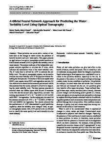
2.6 Plant Root Measurement In the experiments, the plant root depths during the growing season of the Black cumin (Nigella sativa L.) was measured by minirhizotron with 0.50, 0.70 and 1 m depth (Fig. 1).

2.7 Initial Data Processing To improve the training efficiency, the input data should be normal (standard). Entering crude data accuracy and processing speed of the network was reduced as below:

 X  Xmean  Xnormal  0.5  0.5   X max  X min 

(2)

Where Xnormal is the normal of data, Xmean is the groundwater observation means, Xmax and Xmin are the maximum and minimum

362

Ghamarnia and Jalili; JSRR, 7(5): 359-372, 2015; Article no.JSRR.2015.217

groundwater observations, respectively [21]. Daily groundwater uptakes by Black cumin roots were measured throughout 2011-2012 growing season and were compared to simulated values by Artificial Neural Networks data. The qualitative procedure consisted of visually comparing the predicted and measured groundwater uptakes over groundwater depths. The quantitative procedures involved the use of error statistics [22] calculated as below: m

RMSE 

 i  1 S i

M

i

2

(3)

m m

MAE 

 i 1 S i

MBE 

 i  1 S i

Mi

(4)

m m

M

i



3. RESULTS AND DISCUSSION Neural network design needs three sets of training, cross validation, and testing data. In the present study, 40 percent of data were used for education, 40 percent for cross validation and 20 percent to test the network. Multilayer perceptron networks (MLP) can be most applied of artificial neural networks. In this study the multilayer perceptron network with error back propagation learning algorithm was used to predict the rate of water uptake by plant roots groundwater. Levenberg Marquardt, Momentum and Quick Prop learning rule were also used in the study. The selection of the appropriate number of neurons in the hidden layer and the optimal number of replications based on the indicators MSE and R2 were compared.

3.1 Topology of ANN

(5)

m

Fig. 1. A view of lysimeter with minirhizotron [19] Where RMSE is root mean square error (RMSE) between the measured and simulated daily groundwater uptakes, MAE is mean absolute error and MBE is mean bias error between measurement and simulation. Si is the value simulated by Artificial Neural Networks, Mi is the corresponding measured value and m is the number of data on which measurements were taken (m = 540 for Black cumin) [17]. RMSE indicates the discrepancies between the observed and calculated values. The lower RMSE, the more accurate is the prediction.

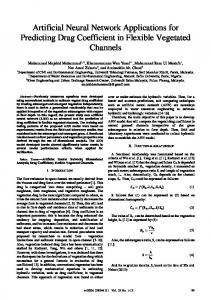
The procedural steps in building ANN model were applied in order to create new ANN model to enable it for prediction of groundwater contribution by input variables [23]. A number of trials were applied to get the best performance. The initial modeling trials were made using all input variables. From created ANN models, the importance and effect of each variable was studied and represented; also, the sensitivity analysis was applied [24]. The predicted values of final groundwater observation were compared to the observed values of groundwater absorption. Several ANN models were created and tested by varying the neural networks type. After a number of trials, the best neural network was determined to be Multilayer Perceptron network (MLP) with four layers: an input layer of 4 neurons, one hidden layer with 4 neurons and the output layer with 1 neuron as shown in Fig. (2). The four input neurons were: total water use evapotranspiration (ETo), root depth (Zr), groundwater salinity (GS) and groundwater depth (Z). The output neuron gives the final groundwater observation (Smax). Fig. (2) presents the topology of the ANN model.

3.2 Total Water Use and Groundwater Contributions A summarized results of the total water used for all nine treatments during the first and second year of the study and those of the related Duncan test classes are given in Table (4). In the first year of the study (2011), the total water use was 650 mm consisting of 167 mm of rainfall, profile storage and 10 mm surface water to help

363

Ghamarnia and Jalili; JSRR, 7(5): 359-372, 2015; Article no.JSRR.2015.217

seedling. The lowest and highest surface water quantities were used for treatments T1 with (0.6, 1 dS/m) and T9 with (1.10, 4 dS/m), respectively. The results of all treatments in the second year of the study (2012) were similar to those in the first year of the study (2011). Because of warmer climate conditions during the early months of the growing season during the second year of study, the total water use for all treatments including 64 mm (rain, profile storage and 10 mm surface water to help seedling) was 708.4 mm. The results in Table (4) show that the lowest and highest surface water amounts used were for treatments T1 (0.60, 1 dS/m) and T9 (1.10, 4 dS/m) [16].

trained for different number of iterations values and mse values were calculated for replication at each stage. Error values and the determination coefficient of the network, with different number of neurons are shown in the Table (6).

3.3 The Number of Initial Replication Selection The hypothetical characteristics in Table (5) were used to determine the number of initial replications. 1000 occurrences were appropriated for network architecture.

3.4 The Number of Hidden Layers and Number of Neurons The next challenge due to size constraints of the eventual model was to determine the total amount of neurons required per layer [25]. After selecting hypothetical network, the network was

Fig. 2. Topology of the ANN model It was expected that a steady increase in neurons per layer would result in the increase of resolution of the fitting pattern of neural network data to the actual observed values. At 8 neurons per layer the data had a sufficiently good fit with an increase of neurons above this level having no real effect on the prediction anymore (see Table 6). After determining the number of occurrences, the number of hidden layer neurons was determined. If the number of hidden layer neurons was to be eight, the minimum error verified and maximum correlation value were obtained [25].

Table 4. Summary of total water, surface, ground water use and groundwater contribution Year

Salinity (dS/m)

Groundwater depth (m)

2011

1

0.60 (T1) 80 (T2).0 1.10 (T3) 0.60 (T4) 80 (T5).0 1.10 (T6) 0.60 (T7) 80 (T8).0 1.10 (T9) 0.60 (T1) 80 (T2).0 1.10 (T3) 0.60 (T4) 80 (T5).0 1.10 (T6) 0.60 (T7) 80 (T8).0 1.10 (T9)

2

4

2012

1

2

4

Total surface water use (mm) 43.4 113 179 83 154 210 133 200 250 175 271 330 220 297 357 259 339 388

Total ground water use (mm) 440 a 370 ab 304 c 400 a 329 c 273.5 d 350 b 283.5 d 234 e 470 a 374 b 315.5 c 425 ab 347.5 c 288 e 386 b 305.5 d 257 e

Rain + profile storage + seedling (mm) 167

Total water use (mm) 650

64

708.4

Groundwater contribution (%) 68 a 57 b 47 c 61.5 ab 51 bc 42 d 54 c 44 d 36 e 66.5 a 53 ab 44.5 c 60 a 49 b 41 d 54.5 b 43 c 36 e

Different letters indicate significant differences at (P