Artificial neural network approach for modelling and ... - ScienceDirect

:~ •

•

? ~ ,"

r,

E(OILOGl(m monLun6 ELSEVIER

Ecological Modelling 96 (1997) 11-28

Artificial neural network approach for modelling and prediction of algal blooms Friedrich Recknagel a, *, Mark French b, Pia Harkonen c, Ken-Ichi Yabunaka d a Department of Environmental Science. University of Adelaide, Roseworthy, Adelaide, South Australia 5371, Australia b Department of Civil Engineering, University of Louisville, Louisville, KY 40292, USA c Laboratory of Hydrology and Water Resources Management, Helsinki University of Teehru~logy, 02150 E~poo, Finland d Department of Chemical Engineering, Tokyo University of Agriculture and Technology, Tokyo 184. Japan Received 22 November 1995; accepted 13 May 1996

Abstract

Following a comparison of current alternative approaches for modelling and prediction of algal blooms, artificial neural networks are introduced and applied as a new, promising model type. The neural network applications were developed and validated by limnological time-series from four different freshwater systems. The water-specific time-series comprised cell numbers or biomass of the ten dominating algae species as observed over up to twelve years and the measured environmental driving variables. The resulting predictions on succession, timing and magnitudes of algal species indicate that artificial neural networks can fit the complexity and nonlinearity of ecological phenomena apparently to a high degree. © 1997 Elsevier Science B.V. Keywords: Blue-green algae; Algal blooms; Modelling; Prediction; Artificial neural networks; Case studies

1. Introduction

Aquatic ecosystems are very complex due the diversity and connections of the components governing the system's dynamics. Nonlinear dynamics underlie the ecosystem behavior and pass it through successional stages aiming at a steady state. This process is more complicated when a single species or substance rapidly increases in number or concentration, whereby they become a pollutant for the ecosystem and can subsequently affect their surroundings drastically.

* Corresponding author. Tel.: +61-8-3037951; fax: +61-83037956.

Explosion-like formations of algal blooms increasingly pollute both: salt and fresh water ecosystems throughout the world. They lead to enormous costs by affecting seafood, drinking water supply, aquaculture systems and tourism. In addition to the characteristics described by Hallegraeff (1993), the following harmful algal blooms can be distinguished: (1) Species which cause water discolorations. Algae can grow in abundance to the extent that they change the color of water to red, brown or green. Resulting water discoloration can significantly impair recreational uses of aquatic systems. In shallow waters, blooms can grow occasionally so dense that they cause, not only water discoloration but also fish and invertebrate mortality due to oxygen depletion. (2) Species which affect human health by toxins.

0304-3800/97/$17.00 Copyright © 1997 Elsevier Science B.V. All rights reserved. PH S0304-3 8 0 0 ( 9 6 ) 0 0 0 4 9 - X

12

F. Recknagel et al./ Ecological Modelling 96 (1997) 11-28

Blue-green algal toxins are contained within the living cells and will be released by cell cracking or decay. The toxins can find their way to humans through either drinking water or the food chain. As reported by Falconer (1993) algal toxins in solution pass through the normal water treatment and are resistent to boiling. They can cause gastroenteritis, hepatoenteritis and toxic injury to the liver. Additionally, the occurrence of fish and shellfish poisonings as reported by Todd (1993) can considerably reduce consumption and export of seafood. (3) Species which cause high mortality offish and invertebrates. Barica (1978) reported massive seasonal mortalities of rainbow trout during summer in Canadian prairie lakes caused by blue-green filamentous algae Aphanizomenonflos-aqua and related degradation products. Some algae species can cause serious damage in aquaculture systems by damming or clogging fish gills. Okaichi (1989) reported on a bloom of Chattonella anfiqua in the Japanese Seto Island Sea which killed 500 million dollars worth of caged yellow-tail fish. (4) Species which impair water treatment by their biomass, taste and odor. A1I Sur face irrsdlenee ater transparency (Zeu) Ix|ng depth (Zm)

Nutrients

gogenic organic matter can seriously impede the supply of drinking water by clogging of filters, inhibition of flocculation processes and encrustation of pipes in water works. Some species such as Synura uvella can cause taste and odor problems in drinking water and give rise to customer complaints (Burlingame et al., 1992). Most of these deleterious effects might be prevented or minimized if algal blooms could be predicted in a early stage. This is a permanent challenge for modelers worldwide. In the context of this paper a comparison of current alternative approaches for modelling and prediction of algal blooms is made. Artificial neural networks are then introduced and applied as a new, promising model type. The neural network applications were developed and validated by limnological time series from freshwater lakes in Japan and Finland and an Australian river. The resulting predictions on succession, timing and magnitudes of algal species indicated that artificial neural networks fit the complexity and nonlinearity of ecological phenomena apparently to a high degree.

Temperature

,o.,o

......

.,..

~

CI~

•

,:,:::,

ql~eomposltlon

t

I

I

CONTROL BY

PHYSIOLOGICAL

LIMITING FACTOR

CONTROL

MULTIFACTORIAL CONTROL

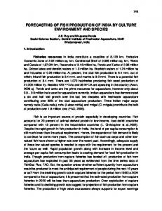
Fig. 1. Factors and processes controlling phytoplankton dynamics (from Capblancq and Catalan, 1994).

F. Recknagel et al. / Ecological Modelling 96 (1997) 11-28

2. Modelling and prediction of phytoplankton in freshwater systems

0

.a2 Z

E

0

~ ~

"=

..i e N N d~

-

:=-

a

,5

-d .-6"~0

:=-

a

~

m

t~

..--

-=

.~

~

.-

E ~ ~

.~ ~

"~ ~ ~-

-_

$ 0

~.

~ ~

- -

"r.

..

_,

-3

fi

i

•=

-- "d

13

.~

~

.~

To model the dynamics of phytoplankton populations, the limiting, physiological and multiple factors controlling their growth and composition have to be considered as represented in Fig. 1. The validity of the model depends upon the availability of either cross-sectional or time-series data and the choice of the modelling technique. Limnological cross-sectional data are obtained from measurements of different lakes (e.g. of equatorial lakes) where each data point represents a seasonally or annually averaged set of measurements for a different lake. Limnological time-series data is composed of a deterministic and a random component. The deterministic component changes over time in a regular and'predictable way caused by underlying processes. It can be characterized by a trend, periodicity and serial dependency. The trend is characterized by the long-term tendency of observations to increase or to decrease, e.g. the increased phosphorus concentrations in lakes due to cultural eutrophication. The periodicity occurs when observations follow a pattern that changes regularly with time, e.g. diurnal changes of oxygen concentration or the seasonal succession of phytoplankton in lakes. The periodicity can be caused by other periodic phenomena such as limit cycles of prey-predator relationships between phytoplankton and zooplankton. The serial dependency occurs when observations in the time series are dependent on past observations, e.g. the phosphorus concentration of lakes in spring depends on the phosphorus level in the previous winter. The random component is superimposed on the deterministic component and can be characterized by shortterm fluctuations due to transitory or unexplained factors. Their nature can be truly random or chaotic. Truly random components such as the level of water in a river can be characterized by a statistical distribution function or by the statistical moments of the data. Chaotic components of a time series are characterized by values that appear to be randomly distributed and non-periodic but are the result of a deterministic process due to underlying nonlinear dynamics. Table ! lists some characteristics of different types of phytoplankton models. Empirical models are

14

F. Recknagel et al./ Ecological Modelling 96 (1997) 11-28

based on cross-section data and predict mean seasonal or annual chlorophyll-a concentrations (e.g. Vollenweider, 1976). They utilize correlative relationships with limiting factors such as water transparency and nutrients. Deterministic models are based on cross-section and time-series data and simulate trends, seasonality and serial dependencies controlled by limiting, physiological and multiple factors. Deterministic ecosystem models calculate the daily biomass of functional algal groups within the pelagic food-web (e.g. Park et al., 1979) while deterministic process models calculate the hourly biomass of separate algae species (e.g. Okada and Aiba, 1983). Time-series analysis models predict time-dependent chlorophyll-a based on multivariate relationships with limiting and multiple factors (e.g. Whitehead and Hornberger, 1984). Heuristic word models predict qualitatively the seasonal dynamics of phytoplankton composition by combining species assemblages with causal knowledge on limiting, physiological and multiple factors (e.g. Sommer et al., 1986). Fuzzy models quantify periodically (e.g. monthly) the possible dominance of algal species (e.g. Recknagel et al., 1994). The possibility of the occurrence of algal species is calculated by membership functions depending on seasons, limiting, physiological and multiple factors. Artificial neural network models are driven by time-series data of algal species and control factors (French and Recknagel, 1994). They allow to predict timing and magnitudes of algal species based upon the strength of

associations with limiting and multiple control factors.

3. T i m e series modelling o f algal b l o o m s by artificial neural n e t w o r k s 3.1. General approach

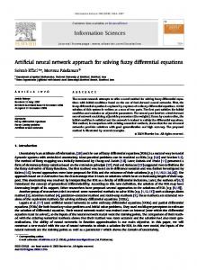
Artificial neural networks typically consist of an input layer, hidden layers and an output layer. In the input layer the external inputs such as surface irradiance and nutrient concentrations, and the density and composition of zooplankton are represented by nodes. In the output layer interesting outputs such as cell numbers of dominating algal species are represented by nodes. Neural networks determine the weighted connections between input and output nodes by interconnected computing elements, the neurons, where feed-forward or feedback algorithms are utilized. The neurons are located in the hidden layers and feed a nonlinear function, such as a sigmoid function, by the sum of its inputs either coming from input nodes by feed-forward or from output nodes by feedback. The resulting value of a neuron is multiplied by a weighting factor after passing the nonlinear function. Therefore each neuron has a separate weight parameter for each connection with the input and output nodes, the so-called firing rate. A learning process, the training, forms the interconnections between the neurons and the nodes. It is accomplished using measured inputs, represented in the

Table 2 Characteristicsof four freshwatersystemsand correspondingneural networkmodels Lake Kasumigaura Lake Biwa(Japan) Lake Tuusulanjaervi (Japan) (Finland) TrophicState hypertrophic meso-/eutrophic eu-/hypertropic Morphometry: - Maximumdepth (m) 7 103 10 - Meandepth(m) 4 41 3.2 - Surfacearea (km2) 220 670 5.95 - Volume(millionm3) 900 27800 19.15 Range of watertemperature(°C) 2.1-32.0 3.3-3 I. 1 0.0-22.4 Mean waterretentiontime(year) 0.55 5.5 0.68 Structureof neural network see Fig. 2 see Fig. 3 see Fig. 4 Time series for training(years) 8 ('84, '85, '87, 6 ('84, '85, '88, 10 ('72, '74, '75, '88, '89, '90, '91, '89, '90, '91) '76, '81, '82, ' 8 3 , '92) '84, '85, '86) Time series for validation(years) 2 ('86, '93) 2 ('86, '87) 2 ('73, '87)

River Darling (Australia) hypertrophic

7.5-29.5 0.002 see Fig. 5 10 ('80-'86, '87-'90, '91-'92) 2 ('86-'87, '90-'91)

F. Recknagel et al. / Ecological Modelling 96 (1997) 11-28

Input Layer

Hidden Layer

OrthoPhosphateImg/ll OV-.-...~W(input) I, I

Nitrate Im~l ~ soco

15

Output Layer

W(output)I. ] ~ ) Microcystisaeruginosa[cells/roll

~

fl:) Oscillatoria[cells/roll

Depth,°,

Phom di.m t.ll

WaterDep ,.I

"

,

Oompho phaena ,l n t

Oxy enl° l

nahaena osa oae oe, n ,

WaterTemperatureI'el C ) ( , , . . ~ ~ x ~

CladoceraDensitylind.al (,~,Y/

/ / / ~

Microcystiswesenbergii[cells/roll

~

,,.,, Cyclotellasp. 1 [cells/roll

CopepodaDensitylind./ll (.y'--~w(inpu0 k. h

W(output)h. °~'X..) Anabaenaaffinis[cells/ml]

Fig. 2. Neural network structure for Lake Kasumigaura (Japan). input layer, and measured outputs, represented in the output layer. The strength of the interconnections is adjusted using an error convergence technique such as the back-propagation algorithm. The aim of the training of a neural network is to minimize the output error with respect to the known desired output. The output error is defined to be the sum of the differences between the network outputs and the measured outputs they are supposed to predict. To meet the aim of minimizing the output error can be supported additionally by optimization techniques such as the method of steepest descent. Once formed by training, the interconnections may remain fixed in Input~yer

the hidden layer and the neural network can be used for predictions. The neural network shell E X P L O R E R from Neural Ware. Inc. (1993) was used for modelling of algal blooms in four different freshwater systems. EXPLORER is a feed-forward network with backpropagation for training. For each of the four applications the hyperbolic function was chosen to calculate the firing rates. The numbers of hidden layers, nodes and neurons as well as learning rates and momenta have been used as control parameters to find optimum training and prediction results. The training of any network involved 500,000 iterations.

Hidden Layer

Output Layer

Ortho Phosphate[mg/l]

~7~ Uroglenaamericana[cells/ml]

Nitrate[mg/l]

Coelastrumcambricum[cells/ml]

DissolvedSilica [mg/l]

•

Secchidepth [m] WaterTemperature[°C]

~