Artificial Neural Network Approach in Radar Target ... - Semantic Scholar

Journal of Computer Science 5 (1): 23-32, 2009 ISSN 1549-3636 © 2009 Science Publications

Artificial Neural Network Approach in Radar Target Classification N.K. Ibrahim, R.S.A. Raja Abdullah and M.I. Saripan Department of Computer and Communications Systems, Faculty of Engineering, University Putra Malaysia, 43400 Serdang Selangor, Malaysia Abstract: Problem statement: This study unveils the potential and utilization of Neural Network (NN) in radar applications for target classification. The radar system under test is a special of it kinds and known as Forward Scattering Radar (FSR). In this study the target is a ground vehicle which is represented by typical public road transport. The features from raw radar signal were extracted manually prior to classification process using Neural Network (NN). Features given to the proposed network model are identified through radar theoretical analysis. Multi-Layer Perceptron (MLP) backpropagation neural network trained with three back-propagation algorithm was implemented and analyzed. In NN classifier, the unknown target is sent to the network trained by the known targets to attain the accurate output. Approach: Two types of classifications were analyzed. The first one is to classify the exact type of vehicle, four vehicle types were selected. The second objective is to grouped vehicle into their categories. The proposed NN architecture is compared to the K Nearest Neighbor classifier and the performance is evaluated. Results: Based on the results, the proposed NN provides a higher percentage of successful classification than the KNN classifier. Conclusion/Recommendation: The result presented here show that NN can be effectively employed in radar classification applications. Key words: Forward scattering radar, neural network, target classification and target recognition INTRODUCTION

signal from the transmitter and the Doppler frequency shift scattered by the moving target. During that time, these forward scatter fences were found to be of very limited use for air defence. Since the coverage area is very narrow, only targets that penetrated a single given fence could be detected. If the target rapidly flew out of that fence it could not be located and tracked. Only when adjacent fences were deployed an approximate position and velocity could be estimated. This problem causes the complex nature of the system. Consequently, most of the early forward scatter fences were eventually replaced by monostatic radars which have better spatial coverage area and location accuracy. On the other hand, FSR offers a number of peculiarities that make it a viable interest. Its’ most attractive feature is the steep rise in the target Radar Cross Section (RCS) compared to traditional monostatic radar[3-6], which improves the sensitivity of the radar system. The forward scattering RCS mainly depends on the target’s physical cross section and the wavelength and is independent of the target’s surface shape as well as to any Radar Absorbing Material (RAM) coating which reduces the target’s RCS in traditional radar[7]. This feature makes FSR robust to stealth technology.

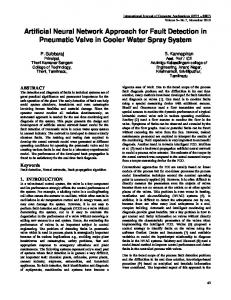
In the Radar System, if the transmitter and receiver are collocated, this configuration is known as a monostatic radar system[1]. In contrast, if the transmitter and receiver are separated, the system is known as a bistatic radar system. The monostatic and bistatic radar system configuration is shown in Fig. 1a and b respectively. Forward Scattering Radar (FSR) is a special type of bistatic radar, where the target is close to the transmitter-receiver baseline as shown in Fig. 1c. FSR presents a conservative class of systems that have a number of fundamental limitations, including the absence of range resolution and operation within narrow angles. Before and during World War II, a so called ‘forward scatter fence’ was used for aircraft detection and almost 200 of these fences were deployed by France, Japan and The Soviet Union[2]. These were bistatic radars, but their geometry was similar to the forward scatter configuration, where targets fly near the transmitter-receiver baseline. These radars used Continuous Wave (CW) transmitters, so the receiver detected a beat frequency produced between the direct

Corresponding Author: RSA Raja Abdullah, Department of Computer and Communications Systems, Faculty of Engineering, University Putra Malaysia, 43400 Serdang Selangor, Malaysia Tel: 603 8946 4347 Fax: 603 8656 7127

23

J. Computer Sci., 5 (1): 23-32, 2009 FSR. So, as far as the authors concern, this is the first research using neural network for automatic target classification in FSR. This research concentrates on developing an automatic classification system to classify target in FSR with the help of NN. Neural Network has found to be a reliable classification tool especially in the image and signal processing. These processing is adopted for the applications such as medical[17-19], machining, power, control and many more. But, only few radar application utilizing NN for classification as well as for other purposes[20-25]. For example, Soleti et al.[20] uses neural network for polarimetric radar target classification. This study shows two different type of feed-forward neural network has been adopted in order to classify the target echo. The networks used have been tested on two types of simulated targets: A small tonnage ship with a low level of detail and medium tonnage ship with higher details. In[21-23], they show the applications of the NN in classifying radar target which used the noisy spectral responses from different types of aircraft to train the network. Their performance are compared with the conventional minimum distance classifier for noisy systems and the NN is found to provide better performance in target classification as compared to a conventional scheme.

R

Transmitter/Receiver

(a)

RR

RT

Transmitter

Receiver

(b) RT

Transmitter

RR

Baseline

Receiver

(c)

MATERIALS AND METHODS

Fig. 1: (a): Monostatic radar (b): Bistatic radar and (c): Forward scattering radar

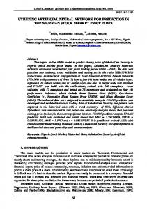
Figure 2 shows the simple FSR radar block diagram and the system topology used for vehicle classification. Detail on the experimental set up, experimentation and data collection can be referred in[8]. In total 850 vehicle signature were collected during the experimentation. The existing FSR system comprises two parts which are the hardware and the software. The hardware includes the two directional antennas (transmitter and receiver) transmitting Continuous Wave (CW) signal. A non-linear component at the receiver selects the Doppler frequency which after low-pass filtering and A/D conversion, are ready for signal processing. The software includes the FFT conversion, pre-processing, feature extraction and classification. The received signal at the receiver contains the direct signal from transmitter and the signal with the Doppler frequency. After it passed through the nonlinear device, Doppler frequency components are extracted which are then used in further signal processing. These signals are in the time domain, then FFT converts the time domain into frequency domain and referred to as the vehicle signature. Figure 3 shows the example of the time domain signal (raw data) and the frequency domain signature. The frequency domain

FSR also requires relatively simple hardware and has a long coherent interval of the received signal. Moreover, FSR receiver can utilise radiation from non-cooperative transmitter without revealing its location. In a hostile environment this is highly desirable as the receiver may be used covertly. All these advantage features create a ‘come back’ interest to FSR. As far as the authors concern only few researcher and research lab seriously working in this area[8-11]. In a number of recent researches, it was shown that FSR can be effectively used for ground target classification[8,12-15]. In these studies, Principal Component Analysis (PCA) is used as the automatic feature extraction and only K-Nearest Neighbor (KNN) is used for the classifier in the proposed FSR system. This method was proved reliable at this stage, but it is necessary to have an alternative classification method as a performance comparison. Thus, this study proposes Neural Network (NN) as the engine for an automatic classification method. The idea was first presented during the International Radar Conference in Edinburgh[16] and it is the first time NN is introduced to 24

J. Computer Sci., 5 (1): 23-32, 2009 signature as in Fig. 3b is the input into pre-processing stage prior to classification using NN. The vehicle signatures obtained from the real FSR outdoor experiment are stored and recorded in the database. Examples of stored vehicle types are showed in Table 1. In Table 1, vehicles are grouped into category based on their physical size. During experimentation, all vehicles passed through the FSR baseline were recorded using a video camera. This allowed us to associate a captured vehicle signature with the respective vehicle. General overview of the proposed automatic classification system is showed in Fig. 4. The system is divided into three parts, which are pre-processing, feature extraction and classification.

(a)

Pre-processing and feature extraction: In the preprocessing stage, the aim is to produce a standard signature before extracting the possible features from the signal. Two normalization processes are applied to all data. In the first process, the frequency domain spectra are normalized to maximum power level and the next one is to normalized to one reference speed.

(b)

Fig. 3: Received signal plot in (a): Time domain and (b): Its frequency domain

Fig. 2: FSR block diagram for vehicle classification

Fig. 4: Proposed automatic classification system Table 1: Vehicle categories with the corresponding car models Number of vehicles ------------------------------------Training Testing Small 15 25

Types of vehicles Peugeot 206

Types of vehicles Ford Focus

Medium

15

15

Mercedes E-class

Honda Accord

Large

15

20

Ford Galaxy

Vauxhall Vivaro

25

J. Computer Sci., 5 (1): 23-32, 2009 In the previous proposed classification system[8], features from the vehicle signature were extracted automatically using PCA prior to classification using KNN. In this study, the features are manually extracted based on the signal theoretical analysis and the common characteristics inherent in the signature. Three features were identified and the detail process is explained. But it is believed that the signatures have more then three attributes as possible features and this is the subject of future researches. As the initial stage, the study only analyses on the three clear significant features. First main lobe width: Each of the vehicle signatures in frequency domain will at least have one common mathematical formula to characterize it. The width of the first main lobe forms a major feature of frequency domain plot and it is given by[8]: ∆f1 =

v l

(a)

(1)

Where: f1 = Main lobe-width v = The velocity of the vehicle l = The maximum length of the vehicle By looking at Eq. 1, obviously f1 will vary and dependent on the speed of the vehicle. This effect causes the received signal cannot directly be used as a feature vector in the classification system. To resolve this, all signatures are scaled to one reference speed. Each new plot to be classified was scaled to the same known speed prior to classification. Figure 5 shows the spectrums of the same vehicle at two different speeds before and after speed normalization for vehicle traveled approximately 9 m sec−1 with a length of 3.6 m. Then first main lobe width, f1 value of these signatures were determined using Eq. 1 and shown in Fig. 6a used as the input to the NN.

(b)

Fig. 5: The frequency spectra of the same car at two different speeds (a): Before speed normalization and (b): After speed normalization Proposed neural network structure: Neural network: NNs are composed of many simple neurons working in parallel to solve the classification problems. Neurons work by processing information. They receive and provide information. The aim of the neural network is to transform the inputs into meaningful outputs. The NN is trained with the available data samples to investigate the relation between inputs and outputs. In this study, backpropagation based Multilayer Perceptron (MLP) network was used. Back propagation is the most common algorithm used to train neural network because of its ability to generalize well on variety of problems. Models built will classify patterns or make predictions according to the patterns of inputs and outputs that have been learned. The learning process consists of two phases, feed-forward and backpropagation. During training, an input is presented to the network and propagates to the output layer, then the output is compared with the desired output and the error is back-propagated so that the weights can be adjusted.

Second main lobe width: By analyzing the signatures, the second characteristics that can be exploited as a feature, is the second main lobe width and shown in Fig. 6b. It is difficult to be determined by an exact formula but at least can be estimated as was proved in[26]. Number of lobes: The next possible feature as the input to the NN is the total number of lobes. Before these numbers can be counted, the first step is to define the threshold frequency (where to set the maximum frequency). Base on experience and wave propagation analysis, the proposed maximum frequency to be processed is 10 Hz. Thus the number of lobe is counted within this limit as shown in Fig. 6c. In this example a program has been created with some rules of determining the number of lobes within 10 Hz. 26

J. Computer Sci., 5 (1): 23-32, 2009

(a)

(a)

(b)

(b)

Fig. 7: MLP network structure (a): Two inputs network and (b): Three inputs network (c)

The first network (NN1) is fed with two inputs and the next model (NN2) is fed with three inputs. Figure 7a and b shows the two proposed network structure. Network structure consists of 3 layers. The input layer consisted of 2 neurons corresponding to our two input features; 1st main lobe-width and 2nd main lobe-width for the first network structure. For the second network, 3 neurons in the input layer corresponding to three input features; 1st and 2nd main lobe-width and the number of lobes. The hidden layer consisted of 10 neurons. The number of neurons in the hidden layer defines by the analysis and it is found that neurons equal to 10 give best results. The number of neurons in the output layer is 4 due to the need to classify the signals into four classes of vehicle. The activation function used in this layer and in the hidden layer is log-sigmoid transfer function. The results will be classified in the range of zeros to ones. It will indicate the confidence of the results.

Fig. 6: Three features used as inputs to NN (a): 1st main lobe-width, (b): 2nd main lobe-width and (c): number of lobes Neural network architecture of the type feed-forward back-propagation (MLP) is used in our approach to classify the FSR signal. This network consists of three layers. The first layer is the input layer which accepts input signals from the outside and redistributes these signals to all neurons in the second layer. The input layer does not include computing neuron. The second layer is the hidden layer. Neurons in the hidden layer detect the features, associated the weights of the neurons in the input patterns. This features then used by the third layer, the output layer in determining the output pattern. This network has three inputs corresponding to the three characteristic extracted from our signal. From these inputs, two network model of NN were built. 27

J. Computer Sci., 5 (1): 23-32, 2009 category of vehicles. The database is created by input the features into NN and NN will set which data were used for training and testing the network model. Training stage: Before training a feed forward network, the weight and biases must be initialized. We used small random values between -0.5 to +0.5 to initialize weights and biases in the network before training. During training, the weights and biases of the network are iteratively adjusted to minimize the network performance function. The default performance function for feed forward networks is mean square errors, the average squared errors between the network outputs and the target output. In the training process, the training data is fed into the input layer. The input features then is propagated to the hidden layer and then to the output layer. This is called the forward pass of the back-propagation algorithm. The output values of the output layer are compared with the target outputs value. If the value is different, an error is calculated and then propagated back toward hidden layer. This is called the backward pass of the back-propagation algorithm. The error is used to update the connection strengths between neuron. The network was trained by using three back-propagation algorithms. Number of epochs is 1000 and the training goal is 0.01. These parameters are used for training both network models. The three algorithms used for training are:

Fig. 8: Vehicle types used in vehicle recognition Table 2: An example of a training data set for recognition 1st main 2nd main Vehicle-type lobe-width lobe-width Vauxhall astra 2.0 3.3 Renault traffic 1.8 3.3 Vauxhall combi 2.1 3.9 Honda civic 2.4 3.6

No. of lobes 7 7 7 6

Table 3: An example of a training data set for categorization 1st main 2nd main Vehicle-category lobe-width lobe-width Small 2.4 3.9 Medium 2.0 3.3 Large 1.8 3.4

No. of lobes 8 7 6

Levenberg-Marquadt (LM) backpropagation algorithm: The LM algorithm was designed to approach second-order training speed without having to compute the Hessian matrix. This algorithm appears to be the fastest method for training moderate-sized feed forward neural network.

Log-sigmoid transfer function: The multilayer networks frequently use the log-sigmoid transfer function. The log-sigmoid function generates outputs between 0 and 1 as the neural network input goes from negative to positive infinity:

Quasi-Newton (BFG) back propagation algorithm: There is a group of algorithms that is based on Newton’s method. The calculation of second derivatives does not require. These are called quasiNewton or secant methods.

Training and testing data: The data recorded during experimentation was used as inputs to the NN. Two types of database were created which is Database 1 for vehicle recognition and Database 2 for vehicle categorization. For vehicle recognition, the system will recognize the exact type of vehicle. Four vehicles from the main database were chosen and Fig. 8 shows the vehicles. Sixty data were used to train the network, 15 from each class of vehicles and the rest are used for testing. Table 2 shows the example of a ‘training data set’ of each type of vehicles. In the vehicle Categorization task, three categories of vehicle have been identified and shown in Table 1. In this task, 45 data were used to train the network, 15 from each category. Table 3 shows an example of a training data set of each

Scaled Conjugate Gradient (SCG) back propagation algorithm: In the Conjugate Gradient (CG), a search is performed along conjugate direction. It produces generally faster convergence than steepest descent directions. Nearly in the entire CG algorithm, the step size is adjusted at each of iteration. A search is made along the conjugate gradient direction to determine the step size, which minimizes the performance function along the line. SCG is fully automated; independent parameters and avoids a time consuming line search[27]. 28

J. Computer Sci., 5 (1): 23-32, 2009 Testing stage: After creating the library, the 160 new data was used to testing the network for vehicle recognition. In vehicle categorization, 60 new data was used. During testing phase, no learning takes place. Weights are not changed. The converged weights that are obtained during the training process are then loaded into the network. The outputs are obtained in a feed forward method. The actual outputs then are compared with the classified one. In order to predict success of classifier, the classification accuracy was calculated by analyzing the information coming from the applications.

Table 4: Test results for each type of vehicle Classification result -------------------------------------------No. of NN1 NN2 testing -------------------------------------Vehicle data True False True False Vauxhall Astra 25 21 4 18 7 Renault Traffic 20 20 0 20 0 Vauxhall Combi 25 19 6 21 4 Honda Civic 30 30 0 30 0

RESULTS AND DISCUSSION Prior to any recognition process, the training time within the NN model using three different algorithms in back-propagation was analyzed. The performance of these algorithms was evaluated by observing the time needed for completing the training session. Figure 9 shows the training time comparison for the different algorithms in vehicle recognition task. From Fig. 9, LM algorithm shows the fastest algorithm completing the training session compared with BFG and SCG, so we just use the LM algorithm in our training network model for vehicle categorization.

Fig. 9: The training time comparison for different algorithms in vehicle recognition

Vehicle recognition: After the training phase, testing with the three back propagation neural network algorithms was established. The new data which has not been used as an input to the trained network was applied to the network for testing the network performance. As mentioned earlier, two neural network models are used to classify the vehicle signals which are NN1 and NN2. For the first model (NN1), two inputs were used to our network structure (the 1st and the 2nd main lobe-width). After the trained network was tested by the data for testing process, the group of Astra was classified correctly with 84% and incorrectly with 16%. The group of Traffic was classified correctly with 100%. Then, the group of Combi was classified correctly with 76% and incorrectly with 24%. Finally, the group of Honda was classified with 100% correct. The results are shown as in Table 4. For the second neural network model (NN2), three inputs were used to our network structure (the 1st, 2nd main lobe-width and the number of lobes). After the trained network was test by the data for testing process, the group of Astra was classified correctly with 72% and incorrectly with 28%. The group of Traffic and Honda was classified correctly with 100. Then the group of Combi was classified correctly with 84% and incorrectly with 16%. Figure 10a show the classification accuracy for each type of vehicle for both network structures.

As we can see from Table 4, for NN1 there were four false classifications in the Astra group, while 21 data signals were correctly recognized as Astra. In the group of Combi, six data was misclassified and 19 data signals were accurately classified as Combi. While for group of Traffic and Honda, there was 100% correct classification was achieved. From the output of the testing network, it shows that there are two types of data misclassification. The groups of Astra and Combi have data misclassified as shown in Table 4. The first type of misclassification is the network was confused which group the signals are. This is because the two vehicles, example for Astra and Combi, their main lobe-width value is very similar to each other as shown in Table 2. So, the network failed to decide which class of the vehicle is. The second type is the network has strongly confident with the class of the vehicle they recognized but it was totally incorrect. As mentioned earlier, because of their similarity in size of vehicle, the network was wrong in classified the correct group of them is. In fact, the vehicle belongs to the other group. The correct classification was achieved when the network has accurately classified the vehicles into their group. As shown in Table 2, the main lobe-width for the group of Honda and Traffic quite different from the other group and the network will simply classify them into their group.

29

J. Computer Sci., 5 (1): 23-32, 2009 Table 5: Vehicle category classification results Classification result -----------------------------------------------No. of NN1 NN2 Vehicle testing --------------------------------------category data True False True False Small 25 25 0 25 0 Medium 15 15 0 15 0 Large 20 19 1 19 1

(a)

(a) (b)

Fig. 10: The classification accuracy for both network models in (a): Vehicle recognition, (b): Vehicle categorization For the NN2 model, Honda and Traffic still achieved 100% correct classification as shown in Table 4. For Astra, false classification was increase to seven and only 18 data has correct classification. But for the group of Combi, 21 data was correctly classified as Combi compare with 19 data when using NN1 model. Only four false classifications in NN2 model for Combi. Based on the performance achieved for the both model, there are small differentiation in terms of classification accuracy. So we can only used 2 features as an input to our NN and the vehicle categorization will only used NN1 model.

(b)

Fig. 11: Performance comparison (a): Vehicle recognition, (b): Vehicle categorization Comparison with previous work (KNN): In the existing research[12], FSR target classification was used PCA with KNN as their classification method. Based on presented result, we made the performance comparison with the proposed classification method. Figure 11a and b shows the comparison between these two classification methods. From this comparison, we can see that proposed classification method gives better performance than the conventional method. In the conventional method, it used KNN as their classifier. In KNN we have to consider some conflicting issues such as the optimal size of the feature. Discriminatory information may be lost in choosing too few features. The dimensionality of the feature space of the extracted feature must be lower. For the better performance in classification, only a small set of features are used. As we can see from Fig. 11b, the accuracy for NN improves more than the conventional method. In

Vehicle categorization: In this part, the goal is to categorize vehicles into one of three conditional vehicle categories which are small, medium and large cars. By using the same network model (NN1 and NN2), with 45 training data, the data was classified into the vehicle categories. The category classification results are shown in Table 5. From these results, we can see that classifier was correct by 100% for small and medium cars and 95% for large cars. Results for the both models are same. Figure 10b shows the graph of classification accuracy for the both network models. There are only one data was misclassified from the overall data. Since the category is depended on the shape of the car, so the network will easily classify them into their category. 30

J. Computer Sci., 5 (1): 23-32, 2009 conventional method, it is difficult to get clear categorization of vehicles and errors mostly occurred between neighboring categories.

7.

CONCLUSION 8.

The result presented shows that neural networks can be effectively employed in FSR as an automatic classifier. The three layer MLP neural network structure that we have built gave very promising results in vehicle recognition and vehicle categorization. 10% of overall data was misclassified in vehicle recognition and only 2% of overall data was misclassified in vehicle categorization. It becomes the limitation to our system. In this study we believe that we have developed an expert system that can be used in FSR signal classification by using artificial neural network. From the comparison with conventional method (PCA), the stated results show that the proposed classification method provides better performance rather than the PCA. So, it is proved that FSR system with NN classification method has a huge potential to be used as an alternative system for target classification. Future research will be focalized on using the ANN for feature extraction and to use the feature extraction from PCA to become an input to neural network.

9.

10. 11.

12. REFERENCES 1. 2. 3.

4.

5. 6.

Skolnik, M.I., 1980. Introduction to Radar Systems. 3rd Edn., McGraw-Hill Book Company, New York, USA., ISBN: 10: 0070579091, pp: 640. Willis, N.J., 2005. Bistatic Radar. 2nd Edn., SciTech Publishing, ISBN: 1891121456, pp: 329. Boyle, R.J., 1994. Comparison of monostatic and bistatic bearing estimation performance for low RCS targets. IEEE Trans. Aerospace Elect. Syst., 30: 962-968. DOI: 10.1109/7.303773 Siegel, K.M., 1958. Bistatic radars and forward scattering. Proceeding of the National Conference on Aeronautical Electronics, May 12-14, Ohio, pp: 286-290. http://siriscollections.si.edu/search/results.jsp?q=National+A eronautical+Electronics+Conference+(Dayton+Ohi o) Glaser, J.I., 1985. Bistatic RCS of complex objects near forward scatter. IEEE Trans. Aerospace Elect. Syst., 1: 70-78. DOI: 10.1109/TAES.1985.310540 Glaser, J.I., 1989. Some results in the bistatic Radar Cross Section (RCS) of complex objects. Proc. IEEE., 77: 639-648. DOI: 10.1109/5.32054

13.

Hiatt, R.E., K.M. Siegel and H. Weil, 1960. Forward scattering of coated objects illuminated by short wavelength radar. Proceeding IRE, Sept. 1960, IEEE Xplore Press, USA., pp: 1630-1636. DOI: 10.1109/JRPROC.1960.287679 Cherniakov, M., R.S.A.R. Abdullah, P. Jancovic, M. Salous and V. Chapursky, 2006. Automatic ground target classification using forward scattering radar. Proceedings of the Radar, Sonar and Navigation, Oct. 2006, pp: 427-437. DOI: 10.1049/ip-rsn:20050028 Blyakhman, A.B. and I.A. Runova, 1999. Forward scattering radiolocation bistatic RCS and target detection. Proceeding of the IEEE Radar Conference, Apr. 1999, pp: 203-208. DOI: 10.1109/NRC.1999.767314 Haykin, S., 1998. Neural Networks: A Comprehensive Foundation. 2nd Edn., Prentice Hall, New York, ISBN: 10: 0132733501, pp: 842. Myakinkov, A.V., 2005. Optimal detection of highvelocity targets in forward scattering radar. Proceeding of the 5th International Conference on Antenna Theory and Techniques, May 24-27, Kyiv, Ukraine, pp: 345-347. DOI: 10.1109/ICATT.2005.1496976 Abdullah, R.S.A.R., M. Cherniakov and P. Jan ovi , 2004. Automatic vehicle classification in forward scattering radar. Proceeding of the 1st International Workshop on Intelligent Transportation, Mar. 2324, Germany, pp: 7-12. http://wit.tuharburg.de/History/WIT2004/Final_Program.html Abdullah, R.S.A.R., M. Cherniakov, P. Jan ovi and M. Salous, 2005. Progress on using principle component analysis in FSR for vehicle classification. Proceeding of the 2nd International Workshop on Intelligent Transportation, Mar. 1516, Germany, pp: 7-12. http://wit.tuharburg.de/History/WIT2005/WIT2005_Program.htm

14. Cherniakov, M., V.V. Chapurskiy, R.S.A. Raja Abdullah, P. Jan ovi and M. Salous, 2004. Shortrange forward scattering radar. Proceeding of the International Radar Conference, Oct. 18-22, France, pp: 322-328. http://www.see.asso.fr/radar2004/programme.php# 3A-BISTA-1 15. Cherniakov, M., R.S.A. Raja Abdullah, P. Jancovic and M. Salous, 2005. Forward scattering micro sensor for vehicle classification. Proceeding of the IEEE International Radar Conference, May 9-12, pp: 184-189. DOI: 10.1109/RADAR.2005.1435816 31

J. Computer Sci., 5 (1): 23-32, 2009 23. Jiang, W., H. Zhang, Q. Lu and Y. Zhou, 2001. Efficient radar target classification using modular neural networks. Proceeding of the International Radar Conference, Oct. 15-18, Beijing China, pp: 1031-1034. DOI: 0-7803-7000-7/01 24. Heerman, P.D. and N. Khazenie, 1992. Classification of multispectral remote sensing data using a back-propagation neural network. IEEE Trans. Geosci. Remote Sens., 30: 81-88. http://ieeexplore.ieee.org/stamp/stamp.jsp?arnumbe r=00124218 25. Hossen, A., F. Al-Wadahi and A.J. Joseph, 2007. Classification of modulation signals using statistical signal characterization and artificial

16. Raja Abdullah, R.S.A., M.I. Saripan and M. Cherniakov, 2007. Neural network based for automatic vehicle classification in forward scattering radar. Proceeding of the IET International Conference on Radar System, Oct. 15-18, Edinburgh, UK., pp: 48. DOI: 10.1049/cp:20070524 17. Guven, A. and S. Kara, 2006. Classification of electro-oculogram signals using artificial neural network. Expert Syst. Appli., 31: 199-205. DOI: 10.1016/j.eswa.2005.09.017 18. Baxt, W.G., 1990. Use of an artificial neural network for data analysis in clinical decision making: The diagnosis of acute coronary occlusion. Neural Comput., 2: 480-489. DOI: 10.1162/neco.1990.2.4.480 19. Baxt, W.G., 1995. Application of artificial neural

neural networks. Eng. Appli. Artif. Intell., 20: 463-472.

DOI: 10.1016/j.engappai.2006.08.004 26. Raja Abdullah, R.S.A. and M. Cherniakov, 2003. Forward scattering radar for vehicles classification. Proceeding of the VehCom International Conference, June 26-27, University of Birmingham, UK., pp: 73-78. http://www.eee.bham.ac.uk/vehcom-2003/ 27. Engin, M., S. Demirag, E.Z. Engin, G. Celebi, F. Ersan, E. Asena and Z. Colakoglu, 2007. The classification of human tremor signals using artificial neural network. Expert Syst. Appli., 33: 754-761. DOI: 10.1016/j.eswa.2006.06.014

networks to clinical medicine. Lancet, 346: 1135-1138.

DOI: 10.1016/S0140-6736(95)91804-3 20. Soleti, R., L. Cantini, F. Berizzi, A. Capria and D. Calugi, 2006. Neural network for polarimetric radar target classification. Proceeding of the Conference on European Signal Processing, Sept. 2006, Florence, Italy. http://www.arehna.di.uoa.gr/Eusipco2006/papers/1 568982306.pdf 21. Chakrabarti, S., N. Bindal and K. Theagharajan, 1995. Robust radar target classifier using artificial neural networks. IEEE Trans. Neural Network, 6: 760-766. DOI: 10.1109/72.377982 22. Jouny, I., F.D. Garber and S.C. Ahalt, 1993. Classification of radar targets using synthetic neural networks. IEEE Trans. Aerospace Elect. Syst., 29: 336-344. http://ieeexplore.ieee.org/ielx5/7/5449/00210072.p df?arnumber=210072

32