artificial neural network-based settlement prediction ...

ARTIFICIAL NEURAL NETWORK−BASED SETTLEMENT PREDICTION FORMULA FOR SHALLOW FOUNDATIONS ON GRANULAR SOILS Mohamed A. Shahin, Mark B. Jaksa and Holger R. Maier School of Civil and Environmental Engineering, The University of Adelaide

ABSTRACT The problem of estimating the settlement of shallow foundations on granular soils is very complex and not yet entirely understood. The geotechnical literature has included many formulae that are based on several theoretical or experimental methods to obtain an accurate, or near-accurate, prediction of such settlement. However, these methods fail to achieve consistent success in relation to accurate settlement prediction. Recently, artificial neural networks (ANNs) have been used successfully for settlement prediction of shallow foundations on granular soils and have been found to outperform the most commonly-used traditional methods. This paper presents a new hand-calculation design formula for settlement prediction of shallow foundations on granular soils based on a more accurate settlement prediction from an artificial neural network model. The design formula presented is a quick tool from which settlement can be calculated easily without the need for computers.

1

INTRODUCTION

The design of shallow foundations on granular soils is generally controlled by settlement rather than bearing capacity. As a consequence, settlement prediction is a major concern and is an essential criterion in the design process of shallow foundations. Consistent and accurate prediction of settlement has yet to be achieved by the use of a variety of methods ranging from purely empirical to complex nonlinear finite elements (Poulos 1999). Comparative studies of the available methods (e.g. Jorden 1977; Jeyapalan and Boehm 1986; Gifford et al. 1987; Tan and Duncan 1991; Wahls 1997) indicate inconsistent prediction of the magnitude of the calculated settlements. This may be attributed to the fact that most of these methods are model driven, in which the form of the model has to be selected in advance, and the unknown model parameters are determined by minimising an error function between model predictions and known historical values. Consequently, prior knowledge regarding the relationship between model inputs and corresponding outputs is needed. In case of settlement of shallow foundations on granular soils, such knowledge is not yet entirely understood. Consequently, model performance may be potentially compromised, as the form of the model chosen may be sup-optimal. In recent times, artificial neural networks (ANNs) have been applied to many geotechnical engineering problems and have demonstrated some degree of success. Recent state-of-the-art ANN applications in geotechnical engineering have been summarised by Shahin et al. (2001). ANNs are a numerical modelling techniques that attempt to simulate the behaviour of the human brain and nervous system. The ANN modelling philosophy is similar to most available methods for settlement prediction in the sense that both are attempting to capture the relationship between a historical set of model inputs and corresponding outputs. However, unlike most available methods, ANNs do not need prior knowledge about the nature of the relationship between the model inputs and corresponding outputs and ANNs, on the other hand, use the data alone to determine the structure of the model as well as the unknown model parameters. This is an essential benefit that enables ANNs to overcome the limitations of the existing methods. A limitation of ANNs, however, is that often the relationships between the input parameters and the outputs are complex and can not be described in a tractable fashion. Recently, Shahin et al. (2002) have used ANNs for settlement prediction of shallow foundations on granular soils and have found that ANNs outperforms three of the most commonly used traditional methods (i.e. Meyerhof 1965; Schultze and Sherif 1973; Schmertmann et al. 1978). The objective of this paper is to derive a practical design formula for settlement prediction of shallow foundations on granular soils based on an ANN model from which settlement can be easily obtained using simple hand calculations.

2

OVERVIEW OF ARTIFICIAL NEURAL NETWORKS

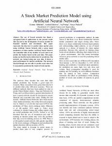
ANNs are a form of artificial intelligence, which by means of their architecture, try to simulate the behaviour of the human brain and nervous system. A comprehensive description of ANNs is beyond the scope of this paper and can be found in many publications (e.g. Hecht-Nielsen 1990; Zurada 1992; Fausett 1994). A typical structure of ANNs consists of a number of processing elements (PEs), or nodes, that are usually arranged in layers: an input layer, an output layer and one or more hidden layers (Figure 1).

Australian Geomechanics – September 2002

45

SETTLEMENT PREDICTION FOR SHALLOW FOUNDATIONS

SHAHIN et al

Figure 1: Structure and operation of an ANN Each PE in a specific layer is fully or partially joined to many other PEs via weighted connections. The input from each PE in the previous layer (xi) is multiplied by an adjustable connection weight (wji). At each PE, the weighted input signals are summed and a threshold value or bias (θj) is added. This combined input (Ij) is then passed through a nonlinear transfer function (f(.)) (e.g. sigmoidal transfer function and tanh transfer function) to produce the output of the PE (yj). The output of one PE provides the input to the PEs in the next layer. This process is summarised in Equations 1 and 2 and illustrated in Figure 1. I j = ∑ w ji xi + θ j

summation

(1)

y j = f (I j )

transfer

(2)

The propagation of information in ANNs starts at the input layer where the network is presented with a historical set of input data and the corresponding (desired) outputs. The actual output of the network is compared with the desired output and an error is calculated. Using this error and utilising a learning rule, the network adjusts its weights until it can find a set of weights that will produce the input/output mapping that has the smallest possible error. This process is called “learning” or “training”. It should be noted that a network with one hidden layer can approximate any continuous function provided that sufficient connection weights are used (Cybenko 1989; Hornik et al. 1989). Once the training phase of the model has been successfully accomplished, the performance of the trained model has to be validated using an independent validation set. Details of the ANN modelling process are beyond the scope of this paper and are given elsewhere (e.g.Moselhi et al. 1992; Flood and Kartam 1994; Maier and Dandy 2000).

3

ANN MODEL DEVELOPMENT FOR SETTLEMENT PREDICTION

The ANN model used to derive the design formula for the present work was developed by Shahin et al. (2002) and uses multilayer perceptrons (MLP) that is trained with the back-propagation training algorithm for feedforward ANNs (Rumelhart et al. 1986). The model has five inputs representing the footing width, B, net applied footing load, q, average blow count, N, obtained using a standard penetration test (SPT) over the depth of influence of the foundation as a measure of soil compressibility, footing geometry (length to width of footing), L/B, and footing embedment ratio (embedment depth to footing width), Df /B. The single model output is foundation settlement, Sm. It should be noted that N is not corrected for overburden pressure or submergence, as recommended by Burland and Burbidge (1985). However, for very fine and silty sand below the water table, the submergence correction proposed by Terzaghi and Peck (1948) when N > 15 is used, as follows: N corrected = 15 + 0.5( N − 15) For gravel or sandy gravel, the correction proposed by Burland and Burbidge (1985) is used, as follows:

(3)

N corrected = 1.25 N (4) It should also be noted that the depth of influence over which N is measured is that proposed by Burland and Burbidge (1985), as follows. When N is decreasing with depth, the depth of influence is taken to be equal to the lesser of 2B or the depth from the bottom of the footing to bedrock. On the other hand, when N is constant or increasing with depth,

46



SHAHIN et al

the depth of influence is taken to be equal to B0.75. Whilst N is far less reliable than other soil compressibility parameters such as those derived from the cone penetration test, unfortunately, the vast majority of published data includes only measurements of N. Despite this shortcoming, as will be demonstrated later, the ANN model is still able to outperform the more traditional methods and provide relatively accurate settlement predictions. The database used for model development comprises a total of 189 individual cases (Shahin et al. 2002). Ranges of the data used for the input and output variables are summarised in Table 1. The available data were divided into three sets (i.e. training, testing and validation) in such a way that they are statistically consistent and thus represent the same Table 1: Ranges of the data used for the ANN model inputs and output Model Variables Footing width, B (m) Net applied footing load, q (kPa) Average SPT blow count, N Footing geometry, L/B Footing embedment ratio, Df /B Measured settlement, Sm (mm)

Minimum value 0.8 18.3 4.0 1.0 0.0 0.6

Maximum value 60.0 697.0 60.0 10.5 3.4 121.0

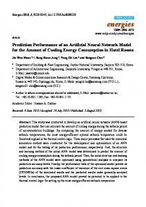
statistical population (Masters 1993). In total, 80% of the data were used for training and 20% were used for validation. The training data were further divided into 70% for the training set and 30% for the testing set. Before presenting the input and output variables for ANN model training, they were scaled between 0.0 and 1.0 to eliminate their dimension and to ensure that all variables receive equal attention during training. The simple linear mapping of the variables’ practical extremes to the neural network’s practical extremes is adopted for scaling as it is the most common method for data scaling (Masters 1993). As part of this method, for each variable x with minimum and maximum values of xmin and xmax, respectively, the scaled value xn is calculated as follows: x n = ( x − x min ) /( x max − x min ) (5) The optimal model geometry was determined utilising a trial-and-error approach in which the ANN models were trained using one hidden layer with 1, 2, 3, 5, 7, 9 and 11 hidden layer nodes, respectively. The optimal network parameters were obtained by training the ANN model with different combinations of learning rates and momentum terms. A model with 2 hidden layer nodes, a learning rate of 0.2, a momentum term of 0.8, tanh transfer function for the hidden layer nodes and sigmoidal transfer function for the output layer node was found to perform best (Shahin et al. 2002). The performance of the model is summarised in Table 2. It can be seen that the model performs well, as it has high correlation coefficients, r, and low root mean squared errors (RMSE) and mean absolute errors (MAE) between the measured and predicted settlements for all data sets (i.e. training, testing and validation). A comparison carried out by Shahin et al. (2002) on the validation set and utilising the ANN model and three traditional methods (i.e. (Meyerhof 1965), (Schultze and Sherif 1973) and (Schmertmann et al. 1978)), indicated that the ANN method provides more accurate settlement predictions than the traditional methods (Table 3). The structure of the optimal ANN model is shown in Figure 2 while its connection weights and threshold levels are summarised in Table 4. Table 2: Performance of the optimal ANN model Data set Training Testing Validation

Correlation coefficient, r 0.930 0.929 0.905

RMSE (mm) 10.01 10.12 11.04

MAE (mm) 6.87 6.43 8.78

Table 3: Performance of ANN and traditional methods for the validation set Performance measure Correlation coefficient, r RMSE MAE

ANN 0.905 11.04 8.78

Meyerhof (1965) 0.440 25.72 16.59

Schultze & Sherif (1973) 0.729 23.55 11.81


Schmertmann et al. (1978) 0.798 23.67 15.69

47


B

1

q

2

N

3

L/B

4

Df /B

5

SHAHIN et al

6 8 7

Sm

Output layer

Hidden layer

Input layer Figure 2: Structure of the optimal ANN model Table 4: Weights and threshold levels for the ANN model Hidden layer nodes j=6 j=7 Output layer nodes j=8

wji (weight from node i in the input layer to node j in the hidden layer ) i=1 i=2 i=3 i=4 i=5 0.227 0.481 0.229 −0.017 0.067 −2.442 −1.114 4.239 −0.498 2.500 wji (weight from node i in the hidden layer to node j in the output layer ) i=6 i=7 0.725 −2.984 -

4

Hidden layer threshold (θj) 0.124 0.188 Output layer threshold (θj) −0.312

THE DESIGN FORMULA

The small number of connection weights of the neural network enables the ANN model to be translated into a relatively simple formula in which the predicted settlement can be expressed as follows: Sp =

1 1+ e

(θ 8 + w86 tanh x1 + w87 tanh x2 )

(6)

where: x1 = θ 6 + w61 B + w62 q + w63 N + w64 ( L / B) + w65 ( D f / B )

(7)

x 2 = θ 7 + w71 B + w72 q + w73 N + w74 ( L / B ) + w75 ( D f / B )

(8)

It should be noted that, before using Equations 7 and 8, all input variables (i.e. B, q, N, L/B and Df /B) need to be scaled between 0.0 and 1.0 using Equation 5 and the data ranges in Table 1. It should also be noted that predicted settlement obtained from Equation 6 is scaled between 0.0 and 1.0 and in order to obtain the actual value, this settlement has to be re-scaled using Equation 5 and the data ranges in Table 1. Such a procedure for scaling and substituting the values of weights and threshold levels from Table 3, Equations 6, 7 and 8 can be rewritten as follows: 120.4   S p = 0.6 +  ( 0.312− 0.725 tanh x1 + 2.984 tanh x2 )  1 e +  

(9)

and

[

] x 2 = 10 −3 [0.7 − 41B − 1.6q + 75 N − 52( L / B) + 740( D f / B)] x1 = 0.1 + 10 −3 3.8B + 0.7q + 4.1N − 1.8( L / B) + 19( D f / B)

where: Sp B

48

= predicted settlement (mm); = footing width (m);


(10) (11)


q N L/B Df /B

SHAHIN et al

= net applied footing load (kPa); = average SPT blow count; = footing geometry; and = footing embedment ratio.

It should be noted that Equation 9 is valid only for the ranges of values of B, q, N, L/B and Df /B given in Table 1. This is due to the fact that ANNs should be used only in interpolation and not extrapolation (Flood and Kartam 1994; Minns and Hall 1996; Tokar and Johnson 1999).

5

SENSITIVITY AND ROBUSTNESS OF THE SETTLEMENT MODEL

120

Predicted settlement (mm)


In order to test the robustness of the predictive ability of the design formula over a range of data valid for Equation 9 (i.e. within the ranges of data shown in Table 1), a sensitivity analysis is carried out. The predicted settlements from Equation 9 are examined against changes to the input variables. All input variables except one are fixed to the mean values of the data shown in Table 1, and a set of synthetic data for the single varied input is generated by increasing the value of this input in increments equal to 5% of the total range between its minimum and maximum values. These inputs are presented to Equation 9 and the predicted settlements are calculated. This process is repeated for all input

100 80 60 40 20 0 0

10

20

30

40

50

60

40 30 20 10 0 0

100


60 50 40 30 20 10 0 0

10

20

30

40

200

300

400

500

600

700

Ne t a pplie d footing loa d (kPa ) (b)

70

50

20 16 12 8 4 0 1

60

2

3

4

5

6

7

8

9

10

Footing ge om e try (d)

Ave ra ge SPT blow count (c)



Footing w idth (m ) (a )

20 16 12 8 4 0 0

0.5

1

1.5

2

2.5

3

3.5

Footing e m be dm e nt ra tio (e )

Figure 3: Results of sensitivity analysis to test robustness of the settlement model


49


SHAHIN et al

N=10 Predicted settlement (mm)


N=5 120 110 100 90 80 70 60 50 40 30 20 10 0

q=20 kPa q=100 kPa q=200 kPa q=300 kPa q=500 kPa q=700 kPa 0

5

10

15

20

25

30

35

40

45

50

55

60

120 110 100 90 80 70 60 50 40 30 20 10 0

q=20 kPa q=100 kPa q=200 kPa q=300 kPa q=500 kPa q=700 kPa

0

5

10

15

20

Footing width (m)

25



q=20 kPa q=100 kPa q=200 kPa q=300 kPa q=500 kPa q=700 kPa 5

10

15

20

25

30

35

40

45

50

55



q=300 kPa q=500 kPa q=700 kPa

20

25

30

q=200 kPa q=300 kPa q=500 kPa q=700 kPa 5

10

15

20

35

40

45

50

55

60

120 110 100 90 80 70 60 50 40 30 20 10 0

25

30

q=300 kPa q=500 kPa q=700 kPa

20

25

30

55

60

40

45

50

55

60

40

45

50

55

60

q=200 kPa q=300 kPa q=500 kPa q=700 kPa

0



q=200 kPa

15

50

5

10

15

20

25

30

35

N=60

q=100 kPa

10

45

Footing width (m)

q=20 kPa

5

40

q=100 kPa

N=50

0

35

q=20 kPa

Footing width (m)

120 110 100 90 80 70 60 50 40 30 20 10 0

60

N=40

q=200 kPa

15

55

Footing width (m)

q=100 kPa

10

50

q=100 kPa

0

60

q=20 kPa

5

45

q=20 kPa

N=30

0

40

120 110 100 90 80 70 60 50 40 30 20 10 0

Footing width (m)

120 110 100 90 80 70 60 50 40 30 20 10 0

35

N=20

N=15 120 110 100 90 80 70 60 50 40 30 20 10 0 0

30

Footing width (m)

35

40

45

50

55

60

120 110 100 90 80 70 60 50 40 30 20 10 0

q=20 kPa q=100 kPa q=200 kPa q=300 kPa q=500 kPa q=700 kPa

0

5

Footing width (m)

10

15

20

25

30

35

Footing width (m)

Figure 4: Illustrative set of design charts based on the settlement formula (L/B = 1.0 and Df /B = 0.0) variables. The robustness of the design formula can be determined by examining how well the predicted settlements are in agreement with the underlying physical behaviour of settlement prediction based on known geotechnical knowledge. Equation 9 is deemed to be robust if the settlement predictions, over a wide range of data, make sense and are represented by smooth and continuous functions. The results of the sensitivity analysis are shown in Figure 3. It can be seen that the direction of the trends are in agreement with what one would expect based on the physical sense of settlement prediction. For example, in Figures

50



SHAHIN et al

3(a), 3(b) and 3(d), respectively, there is an increase in the predicted settlement as footing width, net applied footing load and footing geometry increase, as one would expect. On the other hand, in Figures 3(c) and 3(e), respectively, the predicted settlements decrease as the average SPT blow count and footing embedment ratio increase. This indicates that Equation 9 is robust and can be used for predictive purposes The credibility of predicted settlements using Equation 9 is further investigated graphically by translating the information obtained from the ANN model into a set of design charts. This is carried out by feeding Equation 9 with synthetic input values within the ranges of data shown in Table 1, and the associated settlements are calculated. It was found that the trends of the design charts are in good agreement with what one would expect. Figure 4 is an illustrative sample of the design charts obtained for L/B = 1.0 and Df /B = 0.0. It can be seen that, for each graph and at a certain net applied footing load, settlement increases as the footing width increases, as expected. It can also be seen that, for each graph and at a certain footing width, settlement increases as the net applied footing load increases, also as expected. On the other hand, moving from one graph to another and at the same footing width and net applied footing load, the settlement decreases as the SPT blow count increases, as expected. These results add more confirmation to the robustness and validity of Equation 9 for settlement prediction.

6

NUMERICAL EXAMPLE

A numerical example is provided to better explain the implementation of the settlement formula. A rectangular footing whose dimensions are 2.5 × 4.0 m is founded at a depth equal to 1.5 m below the ground surface. The soil beneath the footing is sand that extends to a depth in excess of two times its width. The net applied load exerted on the footing is 350 kPa and the average SPT blow count over a depth of two times its width is 16. Solution: Given the information provided, then B = 2.5 m; q = 350 kPa; N = 16; L = 4.0 m and Df = 1.5 m. From Equation 10:   1.5   4.0  x1 = 0.1 + 10 −3 3.8 × 2.5 + 0.7 × 350 + 4.1 × 16 − 1.8  = 0.4286  + 19  2.5   2.5   From Equation 11:   4.0   1.5  x 2 = 10 −3 0.7 − 41 × 2.5 − 1.6 × 350 + 75 × 16 − 52  + 740  = 0.8990 2 . 5    2.5   By substituting x1 and x2 in Equation 9, the predicted settlement can be obtained as follows: 120.4   S p = 0.6 +  = 13.2 mm ( 0.312− 0.725 tanh 0.4286+ 2.984 tanh 0.8990)  1 + e 

7

CONCLUSIONS

Current traditional methods have been unable to predict accurately settlements of shallow foundations on granular soils. A recently developed model based on artificial neural networks (ANNs) has been shown to outperform the most commonly-used traditional methods. Because of its parsimonious architecture, the ANN model is able to be translated into a tractable and relatively simple formula which is suitable for hand calculation. The main shortcoming of the ANN-based proposed formula is that since the ANN model is based on data and is suitable for use in an interpolative sense, it may not perform well in all design situations. In addition, like all empirical models, the range of applicability of the ANN-based design formula is constrained by the data used in model calibration phase and in order to update the model and make it more accurate in the future, it would be desirable to include additional data so that the model can be re-trained. If any practitioners have suitable data regarding shallow foundations on granular soils that include settlement measurements, the authors would be grateful to receive such data. Such practitioners may contact Dr. Mark Jaksa ([email protected]).


51


8

SHAHIN et al

REFERENCES

Burland, J. B., and Burbidge, M. C. (1985). “Settlement of foundations on sand and gravel.” Proc. Institution of Civil Engineers, London, 78-Part 1, 1325-1381. Cybenko, G. (1989). “Approximation by superpositions of a sigmoidal function.” Mathematics of Control, Signals, and Systems, 3, 303-314. Fausett, L. V. (1994). Fundamentals neural networks: Architecture, algorithms, and applications, Prentice-Hall, Englewood Cliffs, New Jersey. Flood, I., and Kartam, N. (1994). “Neural networks in civil engineering I: Principles and understanding.” J. Computing in Civil Eng., 8(2), 131-148. Gifford, D. G., Wheeler, J. R., Kraemer, S. R., and McKown, A. F. (1987). “Spread footings for highway bridges.” Final Report, FHWA/RD-86/185, Federal Highway Administration, Washington, DC. Hecht-Nielsen, R. (1990). Neurocomputing, Addison-Wesely Publishing Company, Reading, MA. Hornik, K., Stinchcombe, M., and White, H. (1989). “Multilayer feedforward networks are universal approximators.” Neural Networks, 2, 359-366. Jeyapalan, J. K., and Boehm, R. (1986). “Procedures for predicting settlements in sands.” Proc. Settlement of Shallow Foundations on Cohesionless Soils: Design and Performance, Geotechnical Special Publication No. 5, ASCE, Seattle, Washington, 1-22. Jorden, E. E. (1977). “Settlement in sand - methods of calculating and factors affecting.” Ground Engineering, 10(1), 30-37. Maier, H. R., and Dandy, G. C. (2000). “Applications of artificial neural networks to forecasting of surface water quality variables: Issues, applications and challenges.” Artificial Neural Networks in Hydrology, R. S. Govindaraju and A. R. Rao, eds., Kluwer, Dordrecht, The Netherlands, 287-309. Masters, T. (1993). Practical neural network recipes in C++, Academic Press, San Diego, California. Meyerhof, G. G. (1965). “Shallow foundations.” J. Soil Mech. & Found. Div., 91(SM2), 21-31. Minns, A. W., and Hall, M. J. (1996). “Artificial neural networks as rainfall-runoff models.” Hydrological Sciences Journal, 41(3), 399-417. Moselhi, O., Hegazy, T., and Fazio, P. (1992). “Potential applications of neural networks in construction.” Can. J. Civil Eng., 19, 521-529. Poulos, H. G. (1999). “Common procedures for foundation settlement analysis-Are they adequate?” Proc. 8th Australia New Zealand Conf. on Geomechanics, Hobart, 3-25. Rumelhart, D. E., Hinton, G. E., and Williams, R. J. (1986). “Learning internal representation by error propagation.” Parallel Distributed Processing, D. E. Rumelhart and J. L. McClelland, eds., MIT Press, Cambridge. Schmertmann, J. H., Hartman, J. P., and Brown, P. B. (1978). “Improved strain influence factor diagrams.” J. Geotech. Eng., 104(GT8), 1131-1135. Schultze, E., and Sherif, G. (1973). “Prediction of settlements from evaluated settlement observations for sand.” Proc. 8th Int. Conf. Soil Mechan. & Found. Eng., 1, 225-230. Shahin, M. A., Jaksa, M. B., and Maier, H. R. (2001). “Artificial neural network applications in geotechnical engineering.” Australian Geomechanics, 36(1), 49-62. Shahin, M. A., Maier, H. R., and Jaksa, M. B. (2002). “Predicting settlement of shallow foundations using neural networks.” J. Geotech. & Geoenv. Eng., 128(9), 785-793. Tan, C. K., and Duncan, J. M. (1991). “Settlement of footings on sands-Accuracy and reliability.” Proc. Geotechnical Eng. Congress, Boulde, Colorado, Geotechnical Special publication No. 27, 446-455. Terzaghi, K., and Peck, R. B. (1948). Soil mechanics in engineering practice, John Wiley, New York. Tokar, S. A., and Johnson, P. A. (1999). “Rainfall-runoff modeling using artificial neural networks.” J. Hydrologic Eng., 4(3), 232-239. Wahls, H. E. (1997). “Settlement analysis for shallow foundations on sand.” Proc. 3rd Int. Geotech. Eng. Conf., Cairo, Egypt, 7-28. Zurada, J. M. (1992). Introduction to artificial neural systems, West Publishing Company, St. Paul.

52
