Artificial Neural Network Modelling of Rice Yield ...

Artificial Neural Network Modelling of Rice Yield Prediction in Precision Farming 1

Puteh Saad, 1Shahrul Nizam Yaakob, 1Noraslina Abdul Rahaman,1Shuhaizar Daud, 2 Aryati Bakri, 3Siti Sakira Kamarudin and 1Nurulisma Ismail [email protected], [email protected], [email protected], [email protected], [email protected], [email protected], [email protected], [email protected]

1

Artificial Intelligence and Software Engineering Research Lab, School of Computer & Communication Engineering, Northern University College of Engineering (KUKUM), Blok A, Kompleks Pusat Pengajian, Jalan Kangar-Arau, 02600 Jejawi, Perlis. 2

Faculty of Computer Science and Information System, University Technology Malaysia, 81310 Skudai, Johor 3

Faculty of Information Technology, University Utara Malaysia, 06010 Sintok, Kedah.

Abstract The production of large quantities of rice without jeopardizing the quality has become an urgent economic concern in Malaysia. Many parameters degrade both quality and quantity of rice production. Among them are pests, weeds, diseases, low quality seedlings and maintenance of a suitable water level. Thus as suggestion to increase the rice production, we propose ANN model to be embedded in IDSS. The model may help farmers to predict rice yield given the aforementioned parameters. Two ANN models are evaluated, Back – Propagation Network and Radial Basis Network. The result shows that Radial Basis Network performs better than Back – Propagation Network in terms of training time, accuracy and number of nodes in the hidden layer. Keywords: artificial neural network, crop yield prediction, radial basis function, backpropagation

1.0 Introduction Precision farming is a new method of crop management by which areas of land or crop within a field may be managed by different levels of input depending upon the yield potential of the crop in that particular area of land. Precision farming is an integrated agricultural management system incorporating several technologies such as global positioning system, geographical information system, yield monitor and variable rate technology [1]. Precision farming has the potential to reduce costs through more efficient and effective applications of crop inputs and it can also reduce environmental impacts by allowing farmers to apply inputs only where they are needed at the appropriate rate [2].

Meanwhile, prediction can be considered as one of the oldest crop management activities [3]. Prediction of crops yield like wheat, corn and rice has always been an interesting research area to agro meteorologist and it has become an important economic concern [4]. Rice is the world’s most important food crop and is a primary source of food for more than half of the world’s population [5]. Almost 90% of rice is produced and consumed in Asia, and 96% in developing countries [6]. In Malaysia, Third Agriculture Policy (1998-2010) was established to meet at least 70% of Malaysia’s demand a 5% increase over the targeted 65%. The remaining 30% comes from imported rice mainly from Thailand, Vietnam and China [7]. Raising level of national rice self-sufficiency has become a strategic issue in the agricultural ministry of Malaysia. The numerous problem associated with rice farming include monitoring the status of nutrient soil, maintaining irrigation infrastructures, obtaining quality seedlings, controlling pests, weeds and diseases, and other problems that need to be addressed in order to increase productivity [8]. A yield prediction system has a potential to overcome some of these problems. The ability to predict the future enables the farm managers to take the most appropriate decision in anticipation of that future. Neural network offers exciting possibilities to perform machine learning and prediction. It’s abundantly utilized in performing agriculture prediction task [4][9][10][11]. Safa et. al, 2002 used Backpropagation Network to predict wheat yield using climatic observation data, with a prediction of maximum of 45-60kg/ha. Sudduth et. al, 1996 used neural network to predict soy bean yield based on soil parameters and achieve a testing error of 17.3%. Liu et.

al, 2001 used NN to predict maize yield based on rainfall, soil and other parameters and obtained a testing error of 14.8%, O’Neal et. al, 2002 used Backpropagation Network to predict rice yield based on whether data. This paper evaluates two artificial neural network model which are backpropagation (BP) network model and radial basis function (RBF) network model.

2.0 Artificial Neural Network Modelling of Rice Yield Prediction In this paper, the development of ANN model taken from Figure 2. The development of ANN model consists of 6 steps as refered in [12] of element. In Step 1 the data to be used for training are collected from Muda Agricultural Development Authority (MADA), Kedah, Malaysia ranging from 1995 to 2001that are cover from 4 areas with 27 locations. With two planting season for each year, total of 14 seasons is generated. There are 35 parameters that affect the rice yield. The parameters were classified to 5 groups. There are 3 types of weed; rumpai, rusiga and daun lebar, 3 types of pests; rats, type of worms and bena perang , 3 types of diseases; bacteria (blb & bls),jalur daun merah (jdm) and hawar seludang, one type of lodging and one type of wind paddy, making a total 11 input parameters. In Step 2 the training data need to be identified, and plan must be made for testing the performance of the network. The collected data are separated into training and test sets. 80% is for training and 20% are reserved for testing. From 378 set data that we get

Parameter

1.

2.

Weed

Pests

Numbers

3

3

Name i.Rumpai ii.Rusiga iii.Daun Lebar i.Rats ii.Type of worms iii.Bena Perang

from combining both of the season (season 1 and season 2), 302 set is been used for training and 76 been used for prediction. There are two types of season that influenced the crop yield in Malaysia. Drought season and raining season. But these are undetermined whether it is occurred in season 1 or season 2. So it is depend on the data given for neural network to detect the parameters affected. As an example if the lodging parameters is been detect affected the rice yield, so most probably it is occurred by raining season and if the wind paddy affected the rice yield, it is occurred by drought season. In Step 3 and 4 a network architecture and a learning method are selected. The backpropagation (BP) network architecture for this research shown in Figure 3 and radial basis function (RBF) architecture is in Figure 4. Step 5 is the initialization of the network weights and parameters, followed by modification of the parameters such as momentum, learning rate and number of neuron in the hidden layer as performance feedback is received. Since these are 11 factors that affect yield, hence the number of node in the input layer is 11. The number of node in the output layer is 1 represent rice yield. Several training is done to obtain the suitable number of nodes in the hidden layer,momentum values and learning rate The next procedure, Step 6, is to transform the application data input into the type and format required by neural network. Preprocessing transforms the data to make it suitable for neural network. Three methods are adapted, (i) by min and max, (ii) by mean and standard deviation and (iii) by principal component analysis. It is found that principal component analysis produce the best performance. Figure 5 shows the data that had been preprocessed using principal component analysis. In Step 7 and Step 8, training and prediction are done. Two artificial neural network models are utilized namely; BP network and RBF network. In Step 9, The network system is integrated into the decision support system as the intelligent component that will be used by farmers to predict the rice yield.

3.0 Radial Basis Function Network

3.

i.Bacteria (blb&bls – Hawar Daun Bakteria & Jalur Daun Bakteria) ii.Jalur Daun Merah(jdm) iii.Hawar Seludang

Diseases

3

4. Wind Paddy

1

-

5.

1

-

Lodging

Table 1: List of Input Parameters.

Radial Basis Function (RBF) neural networks is an alternative to the popular Multi Layer Perceptron (MLP) based neural networks that is used in conjunction with back propogation training method for the generation neural network model. RBF neural networks are function approximation models that can be trained by examples to implement a desired input-output mapping[14]. Under most circumstances, the performance of RBF neural networks can match those of back-propogated MLP.

RBF networks differs from MLP networks from a number of characteristics[15] MLP based networks depends on the number of units per layer, RBF based networks requires that the number of radial basis functions use centres and widths of those functions be calculated earlier. RBF networks employs only one hidden layer and MLP networks may have more than one hidden layer. Nodes in MLP networks typically share a common neural model whereas hidden and output nodes in RBF networks are functionally distinct. Another significant difference is that MLP networks construct “global” approximations to non-linear output approximations whereas RBF networks construct “local” inputoutput approximations (Gaussian functions)[15].RBF network is created by adding a neuron to the hidden layer one at a time until the (SSE) in formula reach below the value objective target.

3.1 Training Phase For an equal comparison between RBF and MLP networks, we trained both network using a total of 378 data samples preprocessed earlier using Principal Component Analysis. For the RBF network, the enhanced RBF training method using function was used and as for the MLP network, gradient descent with momentum and adaptive learning backpropogation technique was used.

Figure 2: The Artificial Neural Network Modelling

Figure 1: Collected data from MADA

Figure 3: Neural Network architecture for Rice Yield Prediction

Input Layer

Input Layer

Hidden Layer Hidden Layer

Output Layer Output Layer

3.1.1

A test training was done to a sample of 378 data pre-processed arlier using Principal Component Analysis and the result of the training process is shown in figure 6.

X1

x1

More Efficient Design RBF Networks

Ø1(r) Ø1(r)

X2

Ø2(r)

∑

y

x2 Ø2(r) X 11

∑ Bias

Øh(r)

bias

x 11

y1

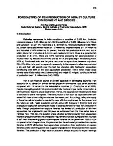
Base on the result, the network requires 365 hundred neurons to be used in the hidden layer before the sum squared error falls below 0.001. Sum squared error(SSE) represent performance of the RBF network. The smaller the SSE value the better network will produce. As shown in Table 2, while network iterated 365 times, the mean square error reached below than 0.001 with the value 0.000994

Øh(r)

Figure 4: Radial Basis Network Architecture

Figure 6: Network performance during training

Figure 5: Data preprocessing using Principal Component Analysis Figure 7: Sum squared error of the RBF network plotted against number of neurons.

The function generates a Resource Allocation Network (RAN) that creates the network by gradually allocating an RBF neuron to the network in the hidden layer until the sum squared error falls below the minimum targeted goal of 0.01 which can lead to a large number of hidden neurons and a very large hidden layer[17],[18]. RBF networks are known to use very large numbers of hidden neurons if used to generate networks that have a multi-dimensional input or output [17]. Because the input samples used for training have 11 input features and 1 output features in it, which can be considered a large multidimensional space, the RBF network tend to use more neurons and takes a considerable amount of training before the final network is generated [17],[18]. This can lead to a low performance and a taxing generation process which is undesirable. From the study, it is found that RBF is unsuitable for multidimensional problems.

3.1.2

Gradient Descent with Momentum and Adaptive Learning Backpropogation

Another test run with the same data, using traingdx (gradient descent) and the result of the training process is shown in figure 8. From the results acquired, it can be seen that the training process on the network using back propogation technique failed to reach 0.001 targets after 5000 epochs. Mean square errors represent network’s performance of the MLP network and have been set to 0.001. The smaller mean square error generate, the better network will produce. As shown in Table 3, after 5000 iterations, mean square error just reaches 0.041227.

References 4.0 Conclusion [1] From the results obtained through training process using both RBF and MLP, it can be clearly seen that MLP networks have a significant disadvantage when paired against RBF results. In training the MLP network, it is often too slow especially in the case of large size problems. Since RBF network can establishes its parameters for hidden neurons directly from the input data and train the network parameters, it is generally much faster compared to MLP network, to complete the training. From the results of the test, RBF based neural network looks more convincing because of the redundancy appeared when using the Multi Layer Perceptron based neural network with back propogation training algorithm on the test samples.

Rains, G.C., and Thomas, D.L., “Precision Farming: An Introduction”, The cooperative extension service, The University of Georgia College of Agricultural and Environmental Sciences, Bulletin 1186, 2002 from http://www.ces.uga.edu/pubcd/b1186.htm [2] Winder, J. and Goddard, T., “About Precision Farming”, Agriculture, Food and Rural Development, Government of Alberta, 2001, from http://www1.agric.gov.ab.ca/$department/deptdocs.nsf/all/sag1 950 [3] Metaxiotis, K. and Psarras, J.,”Expert Systems in Business Applications and Future Directions for the Operations Researcher”, Industrial Management & Data Systems 103/5 361-368 MLB UP Limited, 2003. [4] Safa, B., Khalili, A., Teshnehlab, M. and Liaghat, A., “Prediction of Wheat Yield Using Artificial Neural Networks”, in 25th Conf. on Agricultural and Forest Meteorology, 2002. [5] Khush, G.S., “Harnessing Science and Technology For Sustainable Rice Based Production Systems”, Conf. on Food and Agricultural Organization Rice Conference, 2004. [6] Hossain, M. and Narciso, J., “Global Rice Economy: Long Term Perspectives”, Conf. on Food and Agricultural Organization Rice Conference, 2004. [7] Loh, F. F., “Future of Padi in The Balance”, The Star May 21, 2001, retrieved March 21, 2004, from Koleksi Keratan Akhbar Perputakaan Sultanah Bahiyah UUM.

Figure 8: Network performance during training

[8] MARDI, “Manual Penanaman Padi Berhasil Tinggi Edisi 1/2001”, Malaysian Agriculture research and Development Institute. Malaysian Ministry of Agriculture, 2002. [9] Sudduth, K., Fraisse, C., Drummond, S. and Kitchen, N., “Analysis of Spatial Factors Influencing Crop Yield”, in Proc. Of Int. Conf. on Precision Agriculture, pp. 129-140, 1996. [10] Liu, J., Goering, C.E. and Tian, L., “A Neural Network for Setting Target Corn Yields”, transaction of the ASAE. Vol. 44(3): 705-713, 2001. [11] O’Neal, M.R., Engel, B.A., Ess, D.R. and Frankenberger, J.R., “Neural Network Prediction Of Maize Yield Using Alternative Data Coding Algorithms”, Biosystems Engineering 83(1), 31-45, 2002.

Figure 9: Mean squared error of the MLP network plotted against its epochs

[12] Turban, E.,”Decision Support System and Expert Systems “, Prentice Hall, pp: 694, 1998 [13] Mendelsohn. Lou., “Preprocessing data for neural network”, Stock Market Technologies.

[14] Karayiannis, Nicolaos B., Randolph-Gips, Mary M., “On The Construction and Training of Reformulated Radial Basis Function Neural Networks”, IEEE Transactions on Neural Networks, Vol. 14, July 2003. [15] Carse, B., et. al., “Evolving Radial Basis Function Neural Networks using a Genetic Algorithm”, IEEE International Conference on Evolutionary Computation 1995, Vol. 1, pg. 300, December 1995. [16] K. Na Nakornphanom, Lursinsap, C., Rugchatjaroen, A., “Fault Immunization Model for Elliptic Radial Basis Function Neuron”, Proceedings of the 9th International Conference on Neural Information Processing 2002 (ICONIP’02), Vol. 2, November 2002. [17] Sundararajan, N., Saratchandran, P. and Lu, Y.W.,”Radial Basis Function Neural Networks with Sequential Learning: MRAN and Its Applications”, 1st ed.Singapore: World Scientific, 1999. [18] Alldrin, N., Smith, A. and Trunbull, D.,”Classifying Facial Expression with Radial Basis Function Networks using Gradient Descent and K-Means’, Department of Computer Science, University of California, San Diego, 2003, from http://www.cs.ucsd.edu/~dturnbul/Papers/RBFproject.pdf. [19] Documentation for Math Works Products, Release 14, from http://www.mathworks.com/acces/helpdesk/help/toolbox/nnet/linfilt 6.html.