tions in data mining of neural networks have been multilayer feedforward ... has as many nodes as the number of classes and the output layer node with. 3 ...
Lecture 6
Artificial Neural Networks
1
1
Artificial Neural Networks
In this note we provide an overview of the key concepts that have led to the emergence of Artificial Neural Networks as a major paradigm for Data Mining applications. Neural nets have gone through two major development periods -the early 60’s and the mid 80’s. They were a key development in the field of machine learning. Artificial Neural Networks were inspired by biological findings relating to the behavior of the brain as a network of units called neurons. The human brain is estimated to have around 10 billion neurons each connected on average to 10,000 other neurons. Each neuron receives signals through synapses that control the effects of the signal on the neuron. These synaptic connections are believed to play a key role in the behavior of the brain. The fundamental building block in an Artificial Neural Network is the mathematical model of a neuron as shown in Figure 1. The three basic components of the (artificial) neuron are: 1. The synapses or connecting links that provide weights, wj , to the input values, xj f or j = 1, ...m; 2. An adder that sums the weighted input values to compute the input to the activation function v = w0 +
m �
j=1
wj xj ,where w0 is called the
bias (not to be confused with statistical bias in prediction or estimation) is a numerical value associated with the neuron. It is convenient to think of the bias as the weight for an input x0 whose value is always equal to one, so that v =
m �
j=0
wj xj ;
3. An activation function g (also called a squashing function) that maps v to g(v) the output value of the neuron. This function is a monotone function.
2
Figure 1
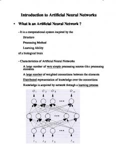
While there are numerous different (artificial) neural network architec tures that have been studied by researchers, the most successful applica tions in data mining of neural networks have been multilayer feedforward networks. These are networks in which there is an input layer consisting of nodes that simply accept the input values and successive layers of nodes that are neurons as depicted in Figure 1. The outputs of neurons in a layer are inputs to neurons in the next layer. The last layer is called the output layer. Layers between the input and output layers are known as hidden layers. Figure 2 is a diagram for this architecture. Figure 2
In a supervised setting where a neural net is used to predict a numerical quantity there is one neuron in the output layer and its output is the predic tion. When the network is used for classification, the output layer typically has as many nodes as the number of classes and the output layer node with 3
the largest output value gives the network’s estimate of the class for a given input. In the special case of two classes it is common to have just one node in the output layer, the classification between the two classes being made by applying a cut-off to the output value at the node.
1.1
Single layer networks
Let us begin by examining neural networks with just one layer of neurons (output layer only, no hidden layers). The simplest network consists of just one neuron with the function g chosen to be the identity function, g(v) = v for all v. In this case notice that the output of the network is
m �
j=0
wj xj , a
linear function of the input vector x with components xj . If we are modeling the dependent variable y using multiple linear regression, we can interpret the neural network as a structure that predicts a value y� for a given input vector x with the weights being the coefficients. If we choose these weights to minimize the mean square error using observations in a training set, these weights would simply be the least squares estimates of the coefficients. The weights in neural nets are also often designed to minimize mean square error in a training data set. There is, however, a different orientation in the case of neural nets: the weights are ”learned”. The network is presented with cases from the training data one at a time and the weights are revised after each case in an attempt to minimize the mean square error. This process of incremental adjustment of weights is based on the error made on training cases and is known as ’training’ the neural net. The almost universally used dynamic updating algorithm for the neural net version of linear regression is known as the Widrow-Hoff rule or the least-mean-square (LMS) algorithm. It is simply stated. Let x(i) denote the input vector x for the ith case used to train the network, and the weights before this case is presented to the net by the vector w(i). The updating rule is w(i+1) = w(i)+η(y(i)−y�(i))x(i) with w(0) = 0. It can be shown that if the network is trained in this manner by repeatedly presenting test data observations one-at-a-time then for suitably small (absolute) values of η the network will learn (converge to) the optimal values of w. Note that the training data may have to be presented several times for w(i) to be close to the optimal w. The advantage of dynamic updating is that the network tracks moderate time trends in the underlying linear model quite effectively. If we consider using the single layer neural net for classification into c classes, we would use c nodes in the output layer. If we think of classical 4
discriminant analysis in neural network terms, the coefficients in Fisher’s classification functions give us weights for the network that are optimal if the input vectors come from Multivariate Normal distributions with a common covariance matrix. For classification into two classes, the linear optimization approach that we examined in class, can be viewed as choosing optimal weights in a single layer neural network using the appropriate objective function. Maximum likelihood coefficients for logistic regression can also be con sidered as weights in a neural network to minimize a function of�the residuals � ev called the deviance. In this case the logistic function g(v) = 1+e is the v activation function for the output node.
1.2
Multilayer Neural networks
Multilayer neural networks are undoubtedly the most popular networks used in applications. While it is possible to consider many activation functions, in practice �it has�been found that the logistic (also called the sigmoid) function ev g(v) = 1+e as the activation function (or minor variants such as the v tanh function) works best. In fact the revival of interest in neural nets was sparked by successes in training neural networks using this function in place of the historically (biologically inspired) step function (the ”perceptron”}. Notice that using a linear function does not achieve anything in multilayer networks that is beyond what can be done with single layer networks with linear activation functions. The practical value of the logistic function arises from the fact that it is almost linear in the range where g is between 0.1 and 0.9 but has a squashing effect on very small or very large values of v. In theory it is sufficient to consider networks with two layers of neurons– one hidden and one output layer–and this is certainly the case for most applications. There are, however, a number of situations where three and sometimes four and five layers have been more effective. For prediction the output node is often given a linear activation function to provide forecasts that are not limited to the zero to one range. An alternative is to scale the output to the linear part (0.1 to 0.9) of the logistic function. Unfortunately there is no clear theory to guide us on choosing the number of nodes in each hidden layer or indeed the number of layers. The common practice is to use trial and error, although there are schemes for combining 5
optimization methods such as genetic algorithms with network training for these parameters. Since trial and error is a necessary part of neural net applications it is important to have an understanding of the standard method used to train a multilayered network: backpropagation. It is no exaggeration to say that the speed of the backprop algorithm made neural nets a practical tool in the manner that the simplex method made linear optimization a practical tool. The revival of strong interest in neural nets in the mid 80s was in large measure due to the efficiency of the backprop algorithm.
1.3
Example1: Fisher’s Iris data
Let us look at the Iris data that Fisher analyzed using Discriminant Analysis. Recall that the data consisted of four measurements on three types of iris flowers. There are 50 observations for each class of iris. A part of the data is reproduced below.
6
OBS# 1 2 3 4 5 6 7 8 9 10 ... 51 52 53 54 55 56 57 58 59 60 ... 101 102 103 104 105 106 107 108 109 110
SPECIES Iris-setosa Iris-setosa Iris-setosa Iris-setosa Iris-setosa Iris-setosa Iris-setosa Iris-setosa Iris-setosa Iris-setosa ... Iris-versicolor Iris-versicolor Iris-versicolor Iris-versicolor Iris-versicolor Iris-versicolor Iris-versicolor Iris-versicolor Iris-versicolor Iris-versicolor ... Iris-virginica Iris-virginica Iris-virginica Iris-virginica Iris-virginica Iris-virginica Iris-virginica Iris-virginica Iris-virginica Iris-virginica
CLASSCODE SEPLEN 1 5.1 1 4.9 1 4.7 1 4.6 1 5 1 5.4 1 4.6 1 5 1 4.4 1 4.9 ... ... 2 7 2 6.4 2 6.9 2 5.5 2 6.5 2 5.7 2 6.3 2 4.9 2 6.6 2 5.2 ... ... 3 6.3 3 5.8 3 7.1 3 6.3 3 6.5 3 7.6 3 4.9 3 7.3 3 6.7 3 7.2
SEPW 3.5 3 3.2 3.1 3.6 3.9 3.4 3.4 2.9 3.1 ... 3.2 3.2 3.1 2.3 2.8 2.8 3.3 2.4 2.9 2.7 ... 3.3 2.7 3 2.9 3 3 2.5 2.9 2.5 3.6
PETLEN 1.4 1.4 1.3 1.5 1.4 1.7 1.4 1.5 1.4 1.5 ... 4.7 4.5 4.9 4 4.6 4.5 4.7 3.3 4.6 3.9 ... 6 5.1 5.9 5.6 5.8 6.6 4.5 6.3 5.8 6.1
If we use a neural net architecture for this classification problem we will need 4 nodes (not counting the bias node) one for each of the 4 independent variables in the input layer and 3 neurons (one for each class) in the output layer. Let us select one hidden layer with 25 neurons. Notice that there will be a total of 25 connections from each node in the input layer to nodes in the hidden layer. This makes a total of 4 x 25 = 100 connections between 7
PETW 0.2 0.2 0.2 0.2 0.2 0.4 0.3 0.2 0.2 0.1 ... 1.4 1.5 1.5 1.3 1.5 1.3 1.6 1 1.3 1.4 ... 2.5 1.9 2.1 1.8 2.2 2.1 1.7 1.8 1.8 2.5
the input layer and the hidden layer. In addition there will be a total of 3 connections from each node in the hidden layer to nodes in the output layer. This makes a total of 25 x 3 = 75 connections between the hidden layer and the output layer. Using the standard logistic activation functions, the network was trained with a run consisting of 60,000 iterations. Each iteration consists of presentation to the input layer of the independent variables in a case, followed by successive computations of the outputs of the neurons of the hidden layer and the output layer using the appropriate weights. The output values of neurons in the output layer are used to compute the er ror. This error is used to adjust the weights of all the connections in the network using the backward propagation (“backprop”) to complete the it eration. Since the training data has 150 cases, each case was presented to the network 400 times. Another way of stating this is to say the network was trained for 400 epochs where an epoch consists of one sweep through the entire training data. The results for the last epoch of training the neural net on this data are shown below: Iris Output 1 Classification Confusion Matrix Desired Class 1 2 3 Total
Computed Class 1 50
2
3
50
49 1 50
1 49 50
Total 50
50
50
150
Patterns 50 50 50 150
# Errors 0 1 1 2
% Errors 0.00 2.00 2.00 1.3
StdDev ( 0.00)
( 1.98)
( 1.98)
( 0.92)
Error Report Class 1 2 3 Overall
The classification error of 1.3% is better than the error using discriminant analysis which was 2% (See lecture note on Discriminant Analysis). Notice that had we stopped after only one pass of the data (150 iterations) the 8
error is much worse (75%) as shown below: Iris Output 2 Classification Confusion Matrix Desired Class 1 2 3 Total
Computed Class 1 2 3 10 7 2 13 1 6 12 5 4 35 13 12
Total 19
20
21
60
The classification error rate of 1.3% was obtained by careful choice of key control parameters for the training run by trial and error. If we set the control parameters to poor values we can have terrible results. To un derstand the parameters involved we need to understand how the backward propagation algorithm works.
1.4
The Backward Propagation Algorithm
We will discuss the backprop algorithm for classification problems. There is a minor adjustment for prediction problems where we are trying to predict a continuous numerical value. In that situation we change the activation function for output layer neurons to the identity function that has output value=input value. (An alternative is to rescale and recenter the logistic function to permit the outputs to be approximately linear in the range of dependent variable values). The backprop algorithm cycles through two distinct passes, a forward pass followed by a backward pass through the layers of the network. The algorithm alternates between these passes several times as it scans the train ing data. Typically, the training data has to be scanned several times before the networks ”learns” to make good classifications. Forward Pass: Computation of outputs of all the neurons in the network The algorithm starts with the first hidden layer using as input values the independent variables of a case (often called an exemplar in the machine learning community) from the training data set. The neuron outputs are computed for all neurons in the first hidden layer by performing 9
the relevant sum and activation function evaluations. These outputs are the inputs for neurons in the second hidden layer. Again the relevant sum and activation function calculations are performed to compute the outputs of second layer neurons. This continues layer by layer until we reach the output layer and compute the outputs for this layer. These output values constitute the neural net’s guess at the value of the dependent variable. If we are using the neural net for classification, and we have c classes, we will have c neuron outputs from the activation functions and we use the largest value to determine the net’s classification. (If c = 2, we can use just one output node with a cut-off value to map an numerical output value to one of the two classes). Let us denote by wij the weight of the connection from node i to node j. The values of wij are initialized to small (generally random) numbers in the range 0.00 ± 0.05. These weights are adjusted to new values in the backward pass as described below. Backward pass: Propagation of error and adjustment of weights This phase begins with the computation of error at each neuron in the output layer. A popular error function is the squared difference between ok the output of node k and yk the target value for that node. The target value is just 1 for the output node corresponding to the class of the exemplar and zero for other output nodes.(In practice it has been found better to use values of 0.9 and 0.1 respectively.) For each output layer node compute its error term as δk = ok (1 − ok )(yk − ok ). These errors are used to adjust the weights of the connections between the last-but-one layer of the network and the output layer. The adjustment is similar to the simple Widrow-Huff rule that we saw earlier in this note. The new value of the weight wjk of the new = w old + ηo δ . Here η is connection from node j to node k is given by: wjk j k jk an important tuning parameter that is chosen by trial and error by repeated runs on the training data. Typical values for η are in the range 0.1 to 0.9. Low values give slow but steady learning, high values give erratic learning and may lead to an unstable network. The process is repeated for the connections between nodes in the last hidden layer and the last-but-one hidden layer. The weight for the connec new = w old + ηo δ where δ = tion between nodes i and j is given by: wij i j j ij � oj (1 − oj ) k wjk δk , for each node j in the last hidden layer. The backward propagation of weight adjustments along these lines con tinues until we reach the input layer. At this time we have a new set of weights on which we can make a new forward pass when presented with a training data observation. 10
1.4.1
Multiple Local Optima and Epochs
The backprop algorithm is a version of the steepest descent optimization method applied to the problem of finding the weights that minimize the error function of the network output. Due to the complexity of the function and the large numbers of weights that are being “trained” as the network “learns”, there is no assurance that the backprop algorithm (and indeed any practical algorithm) will find the optimum weights that minimize error. the procedure can get stuck at a local minimum. It has been found useful to randomize the order of presentation of the cases in a training set between different scans. It is possible to speed up the algorithm by batching, that is updating the weights for several exemplars in a pass. However, at least the extreme case of using the entire training data set on each update has been found to get stuck frequently at poor local minima. A single scan of all cases in the training data is called an epoch. Most applications of feedforward networks and backprop require several epochs before errors are reasonably small. A number of modifications have been proposed to reduce the epochs needed to train a neural net. One commonly employed idea is to incorporate a momentum term that injects some inertia in the weight adjustment on the backward pass. This is done by adding a term to the expression for weight adjustment for a connection that is a frac tion of the previous weight adjustment for that connection. This fraction is called the momentum control parameter. High values of the momentum pa rameter will force successive weight adjustments to be in similar directions. Another idea is to vary the adjustment parameter δ so that it decreases as the number of epochs increases. Intuitively this is useful because it avoids overfitting that is more likely to occur at later epochs than earlier ones. 1.4.2
Overfitting and the choice of training epochs
A weakness of the neural network is that it can be easily overfitted, causing the error rate on validation data to be much larger than the error rate on the training data. It is therefore important not to overtrain the data. A good method for choosing the number of training epochs is to use the validation data set periodically to compute the error rate for it while the network is being trained. The validation error decreases in the early epochs of backprop but after a while it begins to increase. The point of minimum validation error is a good indicator of the best number of epochs for training and the weights at that stage are likely to provide the best error rate in new data.
11
1.5
Adaptive Selection of Architecture
One of the time consuming and complex aspects of using backprop is that we need to decide on an architecture before we can use backprop. The usual procedure is to make intelligent guesses using past experience and to do several trial and error runs on different architectures. Algorithms exist that grow the number of nodes selectively during training or trim them in a manner analogous to what we have seen with CART. Research continues on such methods. However, as of now there seems to be no automatic method that is clearly superior to the trial and error approach.
1.6
Successful Applications
There have been a number of very successful applications of neural nets in engineering applications. One of the well known ones is ALVINN that is an autonomous vehicle driving application for normal speeds on highways. The neural net uses a 30x32 grid of pixel intensities from a fixed camera on the vehicle as input, the output is the direction of steering. It uses 30 output units representing classes such as “sharp left”, “straight ahead”, and “bear right”. It has 960 input units and a single layer of 4 hidden neurons. The backprop algorithm is used to train ALVINN. A number of successful applications have been reported in financial ap plications (see reference 2) such as bankruptcy predictions, currency market trading, picking stocks and commodity trading. Credit card and CRM ap plications have also been reported.
2
References 1. Bishop, Christopher: Neural Networks for Pattern Recognition, Oxford, 1995. 2. Trippi, Robert and Turban, Efraim (editors): Neural Networks in Fi nance and Investing, McGraw Hill 1996.
12