charges having no connection with the real life colour of light. 1 ..... Consider the diagram (e) of figure 1.3, which represents the fermionic loop contribution to the scalar two ...... D40 2987. [82] Ibanez L E and Ross G G 1992 Nucl. Phys. B368 3â37 ...... D22 2227. [98] Chau L L and Keung W Y 1984 Phys. Rev. Lett. 53 1802.
arXiv:1803.06478v1 [hep-ph] 17 Mar 2018
i
Exploring physics beyond the Standard Electroweak Model in the light of supersymmetry
Thesis Submitted to The University of Calcutta for The Degree of Doctor of Philosophy (Science) By
Pradipta Ghosh Advisers: Sourov Roy & Utpal Chattopadhyay
Department of Theoretical Physics Indian Association for the Cultivation of Science Kolkata, India 2011
ii
Abstract Weak scale supersymmetry has perhaps become the most popular choice for explaining new physics beyond the standard model. An extension beyond the standard model was essential to explain issues like gauge-hierarchy problem or non-vanishing neutrino mass. With the initiation of the large hadron collider era at CERN, discovery of weak-scale supersymmetric particles and, of course, Higgs boson are envisaged. In this thesis we try to discuss certain phenomenological aspects of an Rp -violating non-minimal supersymmetric model, called µνSSM. We show that µνSSM can provide a solution to the µ-problem of supersymmetry and can simultaneously accommodate the existing three flavour global data from neutrino experiments even at the tree level with the simple choice of flavour diagonal neutrino Yukawa couplings. We show that it is also possible to achieve different mass hierarchies for light neutrinos at the tree level itself. In µνSSM, the effect of R-parity violation together with a seesaw mechanism with TeV scale right-handed neutrinos are instrumental for light neutrino mass generation. We also analyze the stability of tree level neutrino masses and mixing with the inclusion of one-loop radiative corrections. In addition, we investigate the sensitivity of the one-loop corrections to different light neutrino mass orderings. Decays of the lightest supersymmetric particle were also computed and ratio of certain decay branching ratios was observed to correlate with certain neutrino mixing angle. We extend our analysis for different natures of the lightest supersymmetric particle as well as with various light neutrino mass hierarchies. We present estimation for the length of associated displaced vertices for various natures of the lightest supersymmetric particle which can act as a discriminating feature at a collider experiment. We also present an unconventional signal of Higgs boson in supersymmetry which can lead to a discovery, even at the initial stage of the large hadron collider running. Besides, we show that a signal of this kind can also act as a probe to the seesaw scale. Certain other phenomenological issues have also been addressed.
iii
iv
To a teacher who is like the pole star to me and many others
Dr. Ranjan Ray 1949 - 2001
vi
Acknowledgment I am grateful to the Council of Scientific and Industrial Research, Government of India for providing me the financial assistance for the completion of my thesis work (Award No. 09/080(0539)/2007-EMR-I (Date 12.03.2007)). I am also thankful to my home institute for a junior research fellowship that I had enjoyed from August, 2006 to January, 2007. I have no words to express my gratitude to the members of theoretical high energy physics group of the Department of Theoretical Physics of my home institute, particularly Dr. Utpal Chattopadhyay and Dr. Sourov Roy. Their gratuitous infinite patience for my academic and personal problems, unconditional affection to me, heart-rending analysis of my performance, cordial pray for my success, spontaneous and constant motivations for facing new challenges were beyond the conventional teacherstudent relation. I am also grateful to Dr. Dilip Kumar Ghosh, Dr. Pushan Majumdar, Dr. Koushik Ray, Prof. Siddhartha Sen and Prof. Soumitra SenGupta of the same group for their encouragement, spontaneous affection, crucial guidance and of course criticism, in academics and life beyond it. It is also my pleasure to thank Dr. Shudhanshu Sekhar Mandal and Dr. Krishnendu Sengupta of the condensed matter group. It is an honour for me to express my respect to Prof. Jayanta Kumar Bhattacharjee not only for his marvelous teaching, but also for explaining me a different meaning of academics. I sincerely acknowledge the hard efforts and sincere commitments of my collaborators Dr. Priyotosh Bandopadhyay and Dr. Paramita Dey to the research projects. I am thankful to them for their level of tolerance to my infinite curiosity in spite of their extreme busy schedules. I learned several new techniques and some rare insights of the subjects from them. In the course of scientific collaboration I have been privileged to work with Prof. Biswarup Mukhopadhyaya, who never allowed me to realize the two decades of age difference between us. Apart from his precious scientific guidance (I was also fortunate enough to attend his teaching), his affection and inspiration for me has earned an eternal mark in my memory just like his signature smile. It is my duty to express my sincere gratitude to all of my teachers, starting from the very basic level till date. It was their kind and hard efforts which help me to reach here. I am especially grateful to Ms. Anuradha SenSarma and Mr. Malay Ghosh for their enthusiastic efforts and selfless sacrifices during my school days. I have no words to express my respect to Prof. Anirban Kundu and Prof. Amitava Raychaudhuri for their precious guidance and unconventional teaching during my post-graduate studies. I am really fortunate enough to receive their affection and guidance till date. In this connection I express my modest gratitude to some of the renowned experts of the community for their valuable advise and encouragement. They were always very generous to answer even some of my stupid questions, in spite of their extremely busy professional schedules. I am particularly grateful to Dr. Satyaki Bhattacharya, Prof. Debajyoti Choudhury, Dr. Anindya Datta, Dr. Aseshkrishna Datta, Dr. Manas Maity, Prof. Bruce Mellado, Dr. Sujoy Poddar, Dr. Subhendu Rakshit and Prof. Sreerup Raychaudhuri for many useful suggestions and very helpful discussions. I also express my humble thanks to my home institute, Indian Association for the Cultivation of Science, for providing all the facilities like high-performance personal desktop, constant and affluent access to high-speed internet, a homely atmosphere and definitely a world class library. I am also thankful to all the non-teaching staff members of my department (Mr. Subrata Balti, Mr. Bikash Darji, Mr. Bhudeb Ghosh, Mr. Tapan Moulik and Mr. Suresh Mondal) who were always there to assist us. It is my honour to thank the Director of my home institute, Prof. Kankan Bhattacharyya for the encouragement I received from him. vii
viii It is a pleasure to express my thanks to my colleagues and friends who were always there to cheer me up when things were not so smooth either in academics or in personal life. My cordial and special thanks to Dr. Naba Kumar Bera, Dr. Debottam Das, Sudipto Paul Chowdhury, Dwipesh Majumder and Joydip Mitra who were not just my colleagues but were, are and always will be my brothers. I am really thankful to them and also to Dr. Shyamal Biswas, Amit Chakraborty, Dr. Dipanjan Chakrabarti, Manimala Chakraborty, Sabyasachi Chakraborty, Anirban Datta, Ashmita Das, Sanjib Ghosh, Dr. R. S. Hundi, Dr. Ratna Koley, Dr. Debaprasad Maity, Sourav Mondal, Subhadeep Mondal, Sanhita Modak, Shreyoshi Mondal, Dr. Soumya Prasad Mukherjee, Sutirtha Mukherjee, Tapan Naskar, Dr. Himadri Sekhar Samanta, Kush Saha, Ipsita Saha and Ankur Sensharma for making my office my second home. It is definitely the worst injustice to acknowledge the support of my family as without them I believe it is just like getting lost in crowd. I cannot resist myself to show my humble tribute to three personalities, who by the philosophy of their lives and works have influenced diverse aspects of my life. The scientist who was born long before his time, Richard P. Feynman, the writer who showed that field of expertise is not really a constraint, Narayan Sanyal and my old friend, Mark.
Pradipta Ghosh
List of Publications In refereed journals. • Radiative contribution to neutrino masses and mixing in µνSSM. Pradipta Ghosh, Paramita Dey, Biswarup Mukhopadhyaya, Sourov Roy. Journal of High Energy Physics 05 (2010) 087, arXiv:1002.2705 [hep-ph].
• Neutrino masses and mixing, lightest neutralino decays and a solution to the µ problem in supersymmetry. Pradipta Ghosh, Sourov Roy. Journal of High Energy Physics 04 (2009) 069, arXiv:0812.0084 [hep-ph]. Preprints. • An unusual signal of Higgs boson in supersymmetry at the LHC. Priyotosh Bandyopadhyay, Pradipta Ghosh, Sourov Roy. Phys. Rev. D 84 (2011) 115022, arXiv:1012.5762 [hep-ph]1 . In proceedings. • Neutrino masses and mixing in µνSSM. 2010 J. Phys.: Conf. Ser. 259 012063, arXiv:1010.2578 [hep-ph], PASCOS 2010 • Neutrino masses and mixing in a supersymmetric model and characteristic signatures at the LHC. Proceedings of the XVIII DAE-BRNS symposium, Vol. 18, 2008, 140-143.
1 Now published as “Unusual Higgs boson signal in R-parity violating nonminimal supersymmetric models at the LHC” in Phys. Rev. D 84 (2011) 115022.
ix
x
Motivation and plan of the thesis The standard model of the particle physics is extremely successful in explaining the elementary particle interactions, as has been firmly established by a host of experiments. However, unfortunately there exist certain issues where the standard model is an apparent failure, like unnatural fine tuning associated with the mass of the hitherto unseen Higgs boson or explaining massive neutrinos, as confirmed by neutrino oscillation experiments. A collective approach to address these shortcomings requires extension beyond the standard model framework. The weak scale supersymmetry has been a very favourite choice to explain physics beyond the standard model where by virtue of the construction, the mass of Higgs boson is apparently free from fine-tuning problem. On the other hand, violation of a discrete symmetry called R-parity is an intrinsically supersymmetric way of accommodating massive neutrinos. But, in spite of all these successes supersymmetric theories are also not free from drawbacks and that results in a wide variety of models. Besides, not a single supersymmetric particle has been experimentally discovered yet. Nevertheless, possibility of discovering weak scale supersymmetric particles as well as Higgs boson are highly envisaged with the initiation of the large hadron collider experiment at CERN. In this thesis we plan to study a few phenomenological aspects of a particular variant of R-parity violating supersymmetric model, popularly known as the µνSSM. This model offers a solution for the µ-problem of the minimal supersymmetric standard model and simultaneously accommodate massive neutrinos with the use of a common set of right-handed neutrino superfields. Initially, we aimed to accommodate massive neutrinos in this model consistent with the three flavour global neutrino data with tree level analysis for different schemes of light neutrino masses. Besides, as the lightest supersymmetric particle is unstable due to R-parity violation, we also tried to explore the possible correlations between light neutrino mixing angles with the branching ratios of the decay modes of the lightest supersymmetric particle (which is usually the lightest neutralino for an appreciable region of the parameter space) as a possible check of this model in a collider experiment. Later on we looked forward to re-investigate the tree level analysis with the inclusion of one-loop radiative corrections. We were also keen to study the sensitivity of our one-loop corrected results to the light neutrino mass hierarchy. Finally, we proposed an unconventional background free signal for Higgs boson in µνSSM which can concurrently act as a probe to the seesaw scale. A signal of this kind not only can lead to an early discovery, but also act as an unique collider signature of µνSSM. This thesis is organized as follows, we start with a brief introduction of the standard model in chapter 1, discuss the very basics of mathematical formulations and address the apparent successes and shortcomings. We start our discussion in chapter 2 by studying how the quadratic divergences in the standard model Higgs boson mass can be handled in a supersymmetric theory. We also discuss the relevant mathematical formulations, address the successes and drawbacks of the minimal supersymmetric standard model with special attentions on the µ-problem and the R-parity. A small discussion on the next-to-minimal supersymmetric standard model has also been addressed. We devote chapter 3 for neutrinos. The issues of neutrino mass generation both in supersymmetric and non-supersymmetric models have been addressed for tree level as well as for one-loop level analysis. Besides, implications of neutrino physics in a collider analysis has been discussed. Light neutrino masses and mixing in µνSSM both for tree level and one-loop level analysis are given in chapter 4. The µνSSM model has been discussed more extensively in this chapter. We present the results of correlation study between the neutrino mixing angles and the branching ratios of the decay modes of the lightest neutralino in µνSSM in chapter 5. Our results are given for different natures of the lightest neutralino with different hierarchies in light neutrino masses. Finally, in chapter 6 we present an unusual background xi
xii free signal for Higgs boson in µνSSM, which can lead to early discovery. We list our conclusions in chapter 7. Various technical details, like different mass matrices, couplings, matrix element squares of the three-body decays of the lightest supersymmetric particle, Feynman diagrams etc. are relegated to the appendices.
Contents 1
The Standard Model and beyond... 1.1 The Standard Model . . . . . . . . . . . . . . . . . . . . . . . . . . . . . . . . . . . . . . 1.2 Apparent successes and the dark sides . . . . . . . . . . . . . . . . . . . . . . . . . . . .
2
Supersymmetry 2.1 Waking up to the idea . . . . . . . . . . . . . . . . 2.2 Basics of supersymmetry algebra . . . . . . . . . . 2.3 Constructing a supersymmetric Lagrangian . . . . 2.4 SUSY breaking . . . . . . . . . . . . . . . . . . . . 2.5 Minimal Supersymmetric Standard Model . . . . . 2.6 The R-parity . . . . . . . . . . . . . . . . . . . . . 2.7 Successes of supersymmetry . . . . . . . . . . . . . 2.8 The µ-problem . . . . . . . . . . . . . . . . . . . . 2.9 Next-to-Minimal Supersymmetric Standard Model
. . . . . . . . .
. . . . . . . . .
. . . . . . . . .
. . . . . . . . .
. . . . . . . . .
. . . . . . . . .
. . . . . . . . .
. . . . . . . . .
. . . . . . . . .
. . . . . . . . .
. . . . . . . . .
. . . . . . . . .
. . . . . . . . .
. . . . . . . . .
. . . . . . . . .
. . . . . . . . .
. . . . . . . . .
. . . . . . . . .
. . . . . . . . .
. . . . . . . . .
. . . . . . . . .
13 13 14 16 18 20 25 27 28 29
Neutrinos 3.1 Neutrinos in the Standard Model . . . 3.2 Neutrino oscillation . . . . . . . . . . 3.3 Models of neutrino mass . . . . . . . . 3.3.1 Mass models I . . . . . . . . . 3.3.2 Mass models II . . . . . . . . . 3.4 Testing neutrino oscillation at Collider
. . . . . .
. . . . . .
. . . . . .
. . . . . .
. . . . . .
. . . . . .
. . . . . .
. . . . . .
. . . . . .
. . . . . .
. . . . . .
. . . . . .
. . . . . .
. . . . . .
. . . . . .
. . . . . .
. . . . . .
. . . . . .
. . . . . .
. . . . . .
. . . . . .
41 41 42 47 48 50 58
µνSSM: neutrino masses and mixing 4.1 Introducing µνSSM . . . . . . . . . . . . . . . . . . 4.2 The model . . . . . . . . . . . . . . . . . . . . . . . 4.3 Scalar sector of µνSSM . . . . . . . . . . . . . . . . 4.4 Fermions in µνSSM . . . . . . . . . . . . . . . . . . 4.5 Neutrinos at the tree level . . . . . . . . . . . . . . . 4.5.1 Neutrino masses at the tree level . . . . . . . 4.5.2 Neutrino mixing at the tree level . . . . . . . 4.6 Neutrinos at the loop level . . . . . . . . . . . . . . 4.7 Analysis of neutrino masses and mixing at one-loop 4.8 One-loop corrections and mass hierarchies . . . . . . 4.8.1 Normal hierarchy . . . . . . . . . . . . . . . . 4.8.2 Inverted hierarchy . . . . . . . . . . . . . . . 4.8.3 Quasi-degenerate spectra . . . . . . . . . . . 4.9 Summary . . . . . . . . . . . . . . . . . . . . . . . .
. . . . . . . . . . . . . .
. . . . . . . . . . . . . .
. . . . . . . . . . . . . .
. . . . . . . . . . . . . .
. . . . . . . . . . . . . .
. . . . . . . . . . . . . .
. . . . . . . . . . . . . .
. . . . . . . . . . . . . .
. . . . . . . . . . . . . .
. . . . . . . . . . . . . .
. . . . . . . . . . . . . .
. . . . . . . . . . . . . .
. . . . . . . . . . . . . .
. . . . . . . . . . . . . .
. . . . . . . . . . . . . .
. . . . . . . . . . . . . .
. . . . . . . . . . . . . .
. . . . . . . . . . . . . .
. . . . . . . . . . . . . .
. . . . . . . . . . . . . .
73 73 73 76 78 81 82 83 86 88 91 92 98 100 102
µνSSM: decay of the LSP 5.1 A decaying LSP . . . . . . . . . . . . . . . . . 5.2 Different LSP scenarios in µνSSM . . . . . . . 5.3 Decays of the lightest neutralino in µνSSM . . 5.4 Light neutrino mixing and the neutralino decay
. . . .
. . . .
. . . .
. . . .
. . . .
. . . .
. . . .
. . . .
. . . .
. . . .
. . . .
. . . .
. . . .
. . . .
. . . .
. . . .
. . . .
. . . .
. . . .
. . . .
109 109 109 110 112
3
4
5
. . . . . .
. . . . . .
. . . . . .
xiii
. . . . . .
. . . . . .
. . . . . .
. . . .
. . . . . .
. . . .
. . . .
1 1 6
xiv
CONTENTS 5.4.1 5.4.2 5.4.3
6
7
Bino dominated lightest neutralino . . . . . . . . . . . . . . . . . . . . . . . . . . 113 Higgsino dominated lightest neutralino . . . . . . . . . . . . . . . . . . . . . . . 115 Right-handed neutrino dominated lightest neutralino . . . . . . . . . . . . . . . . 116
µνSSM: Unusual signal of Higgs boson at LHC 6.1 Higgs boson in µνSSM . . . . . . . . . . . . . 6.2 The Signal . . . . . . . . . . . . . . . . . . . 6.3 Collider analysis and detection . . . . . . . . 6.4 Correlations with neutrino mixing angles . . 6.5 Invariant mass . . . . . . . . . . . . . . . . .
. . . . .
. . . . .
. . . . .
. . . . .
. . . . .
. . . . .
. . . . .
. . . . .
. . . . .
. . . . .
. . . . .
. . . . .
. . . . .
. . . . .
. . . . .
. . . . .
. . . . .
. . . . .
. . . . .
. . . . .
. . . . .
. . . . .
. . . . .
. . . . .
Summary and Conclusion
125 125 125 127 130 131 135
A
139 A.1 Scalar mass squared matrices in MSSM . . . . . . . . . . . . . . . . . . . . . . . . . . . 139 A.2 Fermionic mass matrices in MSSM . . . . . . . . . . . . . . . . . . . . . . . . . . . . . . 139
B
141 B.1 Scalar mass squared matrices in µνSSM . . . . . . . . . . . . . . . . . . . . . . . . . . . 141 B.2 Quark mass matrices in µνSSM . . . . . . . . . . . . . . . . . . . . . . . . . . . . . . . . 146
C
147 C.1 Details of expansion matrix ξ . . . . . . . . . . . . . . . . . . . . . . . . . . . . . . . . . 147 C.2 Tree level analysis with perturbative calculation . . . . . . . . . . . . . . . . . . . . . . . 147 C.3 See-saw masses with n generations . . . . . . . . . . . . . . . . . . . . . . . . . . . . . . 149
D
151 D.1 Feynman rules . . . . . . . . . . . . . . . . . . . . . . . . . . . . . . . . . . . . . . . . . 151
E
155 e V function . . . . . . . . . . . . . . . . . . . . . . . . . . . . . . . . . . . . . . . . 155 E.1 The Σ ij e V function . . . . . . . . . . . . . . . . . . . . . . . . . . . . . . . . . . . . . . . . 156 E.2 The Π ij
F G H
I
157 F.1 The B0 , B1 functions . . . . . . . . . . . . . . . . . . . . . . . . . . . . . . . . . . . . . 157 159 G.1 Feynman diagrams for the tree level χ e01 decay . . . . . . . . . . . . . . . . . . . . . . . . 159 161 H.1 Feynman rules . . . . . . . . . . . . . . . . . . . . . . . . . . . . . . . . . . . . . . . . . 161 H.2 Squared matrix elements for h0 → χ e0i χ e0j , b¯b . . . . . . . . . . . . . . . . . . . . . . . . . 163
I.1 I.2 I.3 I.4 I.5 I.6
Three body decays of the χ e01 0 Process χ e1 → q q¯ν . . . . . . − Process χ e01 → `+ i `j νk . . . . 0 Process χ e1 → νi ν j νk . . . . Process χ e01 → u ¯i dj `+ k . . . . 0 Process χ e1 → ui d¯j `− k . . . .
LSP . . . . . . . . . . . . . . .
. . . . . .
. . . . . .
. . . . . .
. . . . . .
. . . . . .
. . . . . .
. . . . . .
. . . . . .
. . . . . .
. . . . . .
. . . . . .
. . . . . .
. . . . . .
. . . . . .
. . . . . .
. . . . . .
. . . . . .
. . . . . .
. . . . . .
. . . . . .
. . . . . .
. . . . . .
. . . . . .
. . . . . .
. . . . . .
. . . . . .
. . . . . .
. . . . . .
. . . . . .
. . . . . .
. . . . . .
165 165 165 170 179 180 184
Chapter 1
The Standard Model and beyond... 1.1 The Standard Model The quest for explaining diverse physical phenomena with a single “supreme” theory is perhaps deeply embedded in the human mind. The journey was started long ago with Michael Faraday and later with James Clerk Maxwell with the unification of the electric and the magnetic forces as the electromagnetic force. The inspiring successful past has finally led us to the Standard Model (SM) (see reviews [1, 2] and [3–6]) of elementary Particle Physics. In the SM three of the four fundamental interactions, namely electromagnetic, weak and strong interactions are framed together. The first stride towards the SM was taken by Sheldon Glashow [7] by unifying the theories of electromagnetic and weak interactions as the electroweak theory. Finally, with pioneering contributions from Steven Weinberg [8] and Abdus Salam [9] and including the third fundamental interaction of nature, namely the strong interaction the Standard Model of particle physics emerged in its modern form. Ever since, the SM has successfully explained host of experimental results and precisely predicted a wide variety of phenomena. Over time and through many experiments by many physicists, the Standard Model has become established as a well-tested physics theory. z The quarks and leptons The SM contains elementary particles which are the basic ingredients of all the matter surrounding us. These particles are divided into two broad classes, namely, quarks and leptons. These particles are called fermions since they are spin 21 particles. Each group of quarks and leptons consists of six members, which are “paired up” or appear in generations. The lightest and most stable particles make up the first generation, whereas the heavier and less stable particles belong to the second and third generations. The six quarks are paired in the three generations, namely the ‘up quark (u)’ and the ‘down quark (d)’ form the first generation, followed by the second generation containing the ‘charm quark (c)’ and ‘strange quark (s)’, and finally the ‘top quark (t)’ and ‘bottom quark (b)’ of the third generation. The leptons are similarly arranged in three generations, namely the ‘electron (e)’ and the ‘electron-neutrino (νe )’, the ‘muon (µ)’ and the ‘muon-neutrino (νµ )’, and the ‘tau (τ )’ and the ‘tau-neutrino (ντ )’. z There are gauge bosons too Apart from the quarks and leptons the SM also contains different types of spin-1 bosons, responsible for mediation of the electromagnetic, weak and the strong interaction. These force mediators essentially emerge as a natural consequence of the theoretical fabrication of the SM, which relies on the principle of local gauge invariance with the gauge group SU(3)C × SU(2)L × U(1)Y . The force mediator gauge bosons are n2 − 1 in number for an SU(n) group and belong to the adjoint representation of the group. The group SU(3)C is associated with the colour symmetry in the quark sector and under this group one obtains the so-called colour triplets. Each quark (q) can carry a colour charge under the SU(3)C group1 (very similar to electric charges under U(1)em symmetry). Each quark carries one of the three 1 The colour quantum number was introduced for quarks [10] to save the Fermi statistics. These are some hypothetical charges having no connection with the real life colour of light.
1
2
CHAPTER 1.
THE STANDARD MODEL AND BEYOND...
fundamental colours (3 representation), namely, red (R), green (G) and blue (B). In a similar fashion an anti-quark (¯ q ) has the complementary colours (¯ 3 representation), cyan (R), magenta (G) and yellow (B). The accompanying eight force mediators are known as gluons (Gaµ ). The gluons belong to the adjoint representation of SU(3)C . However, all of the hadrons (bound states of quarks) are colour singlet. Three weak bosons (Wµa ) are the force mediators for SU(2)L group, under which left-chiral quark and lepton fields transform as doublets. The remaining gauge group U(1)Y provides hypercharge quantum number (Y ) to all the SM particles and the corresponding gauge boson is denoted by Bµ . In describing different gauge bosons the index ‘µ’ (= 1, .., 4) has been used to denote Lorentz index. The index ‘a’ appears for the non-Abelian gauge groups2 and they take values 1, .., 8 for SU(3)C and 1, 2, 3 for SU(2)L . Different transformations for the SM fermions and gauge bosons under the gauge group SU(3)C × SU(2)L × U(1)Y are shown below3 LiL =
�
�
ν`i `i
�
�
L
∼ (1, 2, −1), `iR ∼ (1, 1, −2),
4 2 1 ∼ (3, 2, ), uiR ∼ (3, 1, ), diR ∼ (3, 1, − ), 3 3 3 L Gaµ ∼ (8, 0, 0), Wµa ∼ (1, 3, 0), Bµ ∼ (1, 1, 0), QiL =
ui di
(1.1)
where `i = e, µ, τ , ui = u, c, t and di = d, s, b. The singlet representation is given by 1. z Massive particles in the SM ? Principle of gauge invariance demands for massless gauge bosons which act as the force mediators. In addition, all of the SM fermions (quarks and leptons) are supposed to be exactly massless, as a consequence of the gauge invariance. But these are in clear contradiction to observational facts. In reality one encounters with massive fermions. Also, the short range nature of the weak interaction indicates towards some massive mediators. This apparent contradiction between gauge invariance and massive gauge boson was resolved by the celebrated method of spontaneous breaking of gauge symmetry [12–16]. The initial SM gauge group after spontaneous symmetry breaking (SSB) reduces to SU(3)C ×U(1)em , leaving the colour and electric charges to be conserved in nature. Consequently, the corresponding gauge bosons, gluons and photon, respectively remain massless ensuing gauge invariance, whereas the weak force mediators (W ± and Z bosons) become massive. Symbolically, SU(3)C × SU(2)L × U(1)Y
SSB −−−→ SU(3)C × U(1)em .
(1.2)
Since SU(3)C is unbroken in nature, all the particles existing freely in nature are forced to be colour neutral. In a similar fashion unbroken U(1)em implies that any charged particles having free existence in nature must have their charges as integral multiple of that of a electron or its antiparticle. It is interesting to note that quarks have fractional charges but they are not free in nature since SU(3)C is unbroken. � Spontaneous symmetry breaking Let us consider a Hamiltonian H0 which is invariant under some symmetry transformation. If this symmetry of H0 is not realized by the particle spectrum, the symmetry is spontaneously broken. A more illustrative example is shown in figure 1.1. Here the minima of the potential lie on a circle (white dashed) rather than being a specific point. Each of these points are equally eligible for being the minimum and whenever the red ball chooses a specific minimum, the symmetry of the ground state (the state of minimum energy) is spontaneously broken. In other words, when the symmetry of H0 is not respected by the ground state, the symmetry is spontaneously broken. It turns out that the degeneracy in the ground state is essential for spontaneous symmetry breaking. 2 Yang
and Mills [11]. choose Q = T3 + Y2 , where Q is the electric charge, T3 is the third component of the weak isospin (± 21 for an SU(2) doublet) and Y is the weak hypercharge. 3 We
1.1. THE STANDARD MODEL
3
Figure 1.1: Spontaneous breaking of symmetry through the choice of a specific degenerate ground state. Everything seems to work fine with the massive gauge bosons. But the demon lies within the method of spontaneous symmetry breaking itself. The spontaneous breakdown of a continuous symmetry implies the existence of massless, spinless particles as suggested by Goldstone theorem.4 They are known as Nambu-Goldstone or simply Goldstone bosons. So the SSB apart from generating gauge boson masses also produces massless scalars which are not yet experimentally detected. This is the crisis point when the celebrated “Higgs-mechanism”5 resolves the crisis situation. The unwanted massless scalars are now eaten up by the gauge boson fields and they turn out to be the badly needed longitudinal polarization mode for the “massive” gauge bosons. So this is essentially the reappearance of three degrees of freedom associated with three massless scalars in the form of three longitudinal polarization modes for the massive gauge bosons. This entire mechanism happens without breaking the gauge invariance of the theory explicitly. This mechanism for generating gauge boson masses is also consistent with the renormalizability of a theory with massive gauge bosons.6 The fermion masses also emerge as a consequence of Higgs mechanism. z Higgs sector of the SM and mass generation So the only scalar (spin-0) in the SM is the Higgs boson. Higgs mechanism is incorporated in the SM through a complex scalar doublet Φ with the following transformation properties under the SM gauge group.
Φ=
�
φ+ φ0
�
∼ (1, 2, 1).
(1.3)
The potential for Φ is written as V (Φ) = µ2 Φ† Φ + λ(Φ† Φ)2 ,
(1.4)
with µ2 < 0 and λ > 0 (so that the potential is bounded from below). Only a colour and charge (electric) neutral component can acquire a vacuum expectation value (VEV), since even after SSB the theory remains invariant under SU(3)C × U(1)em (see eqn.(1.2)). Now with a suitable choice of gauge (“unitary gauge”), so that the Goldstone bosons disappear one ends up with � � 1 0 , (1.5) Φ= √ v + h0 2 where h0 is the physical Higgs field and ‘v’ is the VEV for Re(φ0 ) (all other fields acquire zero VEVs) 2 with v 2 = − µλ . At this moment it is apparent that eqn.(1.2) can be recasted as SU(2)L × U(1)Y 4 Initially
SSB −−−→ U(1)em ,
(1.6)
by Nambu [17], Nambu and Jona-Lasino. [18, 19]. General proof by Goldstone [20, 21]. actual name should read as Brout-Englert-Higgs-Guralnik-Hagen-Kibble mechanism after all the contributors. Brout and Englert [13], Higgs [14, 15], Guralnik, Hagen and Kibble [16]. 6 Veltman and ’t Hooft, [22, 23]. 5 The
4
CHAPTER 1.
THE STANDARD MODEL AND BEYOND...
which is essentially the breaking of the electroweak symmetry since the SU(3)C sector remains unaffected. Thus the phenomena of SSB in the context of the SM is identical with the electroweak symmetry breaking (EWSB). The weak bosons, Wµa and U(1)Y gauge boson Bµ now mix together and finally yield three massive vector bosons (Wµ± , Zµ0 ) and one massless photon (A0µ ): Wµ1 ∓ iWµ2 √ , 2 Zµ0 = cosθW Wµ3 − sinθW Bµ , Wµ± =
A0µ = sinθW Wµ3 + cosθW Bµ ,
(1.7)
where θW is the Weinberg angle or weak mixing angle.7 In terms of the SU(2)L and U(1)Y gauge couplings (g2 , g1 ) one can write g2 sinθW = g1 cosθW .
(1.8)
The Wµ± , Zµ0 boson masses are given by MW =
g2 v , 2
MZ =
v 2
2
q g12 + g22 ,
(1.9)
with v 2 = − µλ . The mass of physical Higgs boson (h0 ) is given by m2h0 = 2v 2 λ. Note that mh0 > 0 2 and MZ2 cos2 θW is equal to one at the tree level since µ2 < 0. Interestingly, ratio of the quantities MW (see eqns. (1.8) and (1.9)). This ratio is defined as the ρ-parameter, which is an important parameter for electroweak precision test: ρ=
2 MW 2 MZ cos2 θW
= 1.
(1.10)
There exists an alternative realization of the ρ-parameter. The ρ-parameter specifies the relative strength of the neutral current (mediated through Z-bosons) to the charged current (mediated through W ± -boson) weak interactions. For the purpose of fermion mass generation consider the Lagrangian containing interactions between Higgs field and matter fermions. ˜ i + Hermitian conjugate, −LYukawa = y`i Li Φei + ydi Qi Φdi + yui Qi Φu
(1.11)
where y`i ,ui ,di are the Yukawa couplings for the charged leptons, up-type quarks and down-type quarks, respectively. The SU(2)L doublet and singlet quark and lepton fields are shown in eqn.(1.1). The field ˜ is used to generate masses for the up-type quarks and it is given by Φ � �� − � � ∗ � φ 0 −i −φ0 ∗ ˜ . (1.12) Φ = −iσ2 Φ = i = ∗ i 0 φ0 φ− The fermion masses and their interactions with Higgs field emerge after the EWSB using eqn.(1.11). For example considering the electron these terms are as follows Lelectron Yukawa = − where eL = PL Le (see eqn.(1.1)). So with four component spinor e as
�
ye (v + h0 ) √ (eL eR + eR eL ), 2 eL eR
�
(1.13)
, eqn.(1.13) can be rewritten as
Lelectron Yukawa = −me ee −
me eeh0 , v
(1.14)
with me = Y√e2v as mass of the electron. The particle spectrum of the SM can be written in a tabular form as shown in table 1.1. 7
At present sin2 θW = 0.231 (evaluated at MZ with renormalization scheme M S) [24].
1.1. THE STANDARD MODEL
5
Particle
mass in GeV
Spin
Electric Charge
Colour charge
electron (e) muon (µ)
5.109×10⁻⁴ 0.105
-1 -1
0 0
top-quark (t)
172.0
bottom-quark (b)
4.19
1 2 1 2 1 2 1 2 1 2 1 2 1 2 1 2 1 2 1 2
W-boson (W ± )
80.399
1
Z-boson (Z 0 )
91.187
1
tau (τ )
1.776
neutrinos (νe,µ,τ )
0
up-quark (u)
2.49×10⁻³
down-quark (d)
5.05×10⁻³
charm-quark (c)
1.27
strange-quark (s)
0.101
-1
0
0
0
2 3 − 13 2 3 − 13 2 3 − 13
yes
0
0
±1
yes yes yes yes yes 0
photon (γ)
0
1
0
0
gluon (g)
0
1
0
yes
Higgs (h0 )
?
0
0
0
Table 1.1: The particle spectrum of the SM [24]. Each of the charged particles are accompanied by charge conjugate states of equal mass. The charge neutral particles act as their own antiparticles with all charge like quantum numbers as opposite to that of the corresponding particles. Evidence for Higgs boson is yet experimentally missing and thus Higgs mass is denoted as ‘?’. The neutrinos are presented with zero masses since we are considering the SM only (see section 1.2). z SM interactions Based on the discussion above, the complete Lagrangian for the SM can be written as LSM = L1 + L2 + L3 + L4 ,
(1.15)
where 1. L1 is the part of the Lagrangian which contains kinetic energy terms and self-interaction terms for the gauge bosons. After the EWSB these gauge bosons are known as W ± , Z 0 , gluons and photon. So we have " # 4 8 3 X 1 X a µν 1 X i 1 µν µν L1 = − G G − W W − Bµν B , (1.16) 4 a=1 µν a 4 i=1 µν i 4 µ,ν=1 where Gaµν = ∂µ Gaν − ∂ν Gaµ − g3 fabc Gbµ Gcν ,
i Wµν = ∂µ Wνi − ∂ν Wµi − g2 �ijk Wµj Wνk ,
Bµν = ∂µ Bν − ∂ν Bµ ,
(1.17)
with fabc and �ijk as the structure constants of the respective non-Abelian groups. g3 is the coupling constant for SU(3)C group. 2. Kinetic energy terms for quarks and leptons belong to L2 . This part of the Lagrangian also contains the interaction terms between the elementary fermions and gauge bosons. Symbolically, L2 = iχL D 6 χL + iχR D 6 χR ,
(1.18)
where D 6 = γ µ Dµ with Dµ as the covariant derivative.8 The quantity χL stands for lepton and quark SU(2)L doublets whereas χR denotes SU(2)L singlet fields (see eqn.(1.1)). The covariant 8 Replacement of ordinary derivative (∂ ) by D is essential for a gauge transformation, so that D ψ transforms µ µ µ covariantly under gauge transformation, similar to the matter field, ψ.
6
CHAPTER 1.
THE STANDARD MODEL AND BEYOND...
derivative Dµ for different fermion fields are written as (using eqn.(1.1)) " # 3 X 1 1 i Dµ Qi = ∂µ + ig1 Bµ + i g2 σi .Wµ Qi , 6 2 i=1 � � 2 Dµ ui = ∂µ + ig1 Bµ ui , 3 � � 1 Dµ di = ∂µ − ig1 Bµ di , 3 # " 3 X 1 1 Dµ Li = g2 σi .Wµi Li , ∂µ − ig1 Bµ + i 2 2 i=1 Dµ ei
=
[∂µ − ig1 Bµ ] ei .
(1.19)
But these are the information for SU(2)L × U(1)Y only. What happens to the SU(3)C part? Obviously, for the leptons there will be no problem since they are SU(3)C singlet after all (see eqn.(1.1)). For the quarks the SU(3)C part can be taken care of in the following fashion, " # q 8 qi R iR X 1 (1.20) ∂µ + i g3 λa .Gaµ qi G , Dµ qi G = 2 a=1 qi B qi B where R, G and B are the three types of colour charge and λa ’s are eight Gell-Mann matrices. qi is triplet under SU(3)C , where ‘i’ stands for different types of left handed or right handed (under SU(2)L ) quark flavours, namely u, d, c, s, t and b.
3. The terms representing physical Higgs mass and Higgs self-interactions along with interaction terms between Higgs and the gauge bosons are inhoused in L3 L3 = (Dµ Φ)† (Dµ Φ) − V (Φ).
(1.21)
The expressions for Φ and V (Φ) are given in eqns.(1.3) and (1.4), respectively. For Φ the covariant derivative Dµ is given by " # 3 X 1 1 i Dµ Φ = ∂µ + ig1 Bµ + i g2 σi .Wµ Φ. (1.22) 2 2 i=1 4. The remaining Lagrangian L4 contains lepton and quark mass terms and their interaction terms with Higgs field (h0 ) (after EWSB). The expression for L4 is shown in eqn.(1.11). The elementary fermions get their masses through respective Yukawa couplings, which are free parameters of the theory. It turns out that in the SM the flavour states are not necessarily the mass eigenstates, and it is possible to relate them through an unitary transformation. In case of the quarks this matrix is known as the CKM (Cabibbo-Kobayashi-Maskawa) [25, 26] matrix. This 3 × 3 unitary matrix contains three mixing angles and one phase. The massless neutrinos in the SM make the corresponding leptonic mixing matrix a trivial one (Identity matrix). All possible interactions of the SM are shown in figure 1.2. The loops represent self-interactions like h0 h0 h0 , h0 h0 h0 h0 (from the choice of potential, see eqn. (1.4)) W ± W ± W ∓ W ∓ , ggg or gggg (due to non-Abelian interactions) and also interactions like W ± W ∓ ZZ, W ± W ∓ γγ, W ± W ∓ Z, W ± W ∓ γ etc.
1.2 Apparent successes and the dark sides The SM is an extremely successful theory to explain a host of elementary particle interactions. Masses of the W ± and Z bosons as predicted by the SM theory are very close to their experimentally measured values. The SM also predicted the existence of the charm quark from the requirement to suppress
1.2. APPARENT SUCCESSES AND THE DARK SIDES
7
Figure 1.2: Interactions of the Standard Model. See text for more details. flavour changing neutral current (FCNC)9 before it was actually discovered in 1974. In a similar fashion the SM also predicted the mass of the heavy top quark in the right region before its discovery. Besides, all of the SM particles except Higgs boson have been discovered already and their masses are also measured very precisely [24]. Indeed, apart from Higgs sector, rest of the SM has been already analysed for higher order processes and their spectacular accuracy as revealed by a host of experiments has firmly established the success of the SM. Unfortunately, the so-called glorious success of the SM suffers serious threat from various theoretical and experimental perspective. One of the main stumbling blocks is definitely the Higgs boson, yet to be observed in an experiment and its mass. Some of these shortcomings are listed below. 1. The SM has a large number of free parameters (19). The parameters are 9 Yukawa couplings (or elementary fermion masses) + 3 angles and one phase of CKM matrix + 3 gauge couplings g1 , g2 , g3 10 + 2 parameters (µ, λ) from scalar potential (see eqn.(1.4)) + one vacuum angle for quantum chromodynamics (QCD). The number of free parameters is rather large for a fundamental theory. 2. There are no theoretical explanation why there exist only three generations of quarks and leptons. Also the huge mass hierarchy between different generations (from first to third), that is to say why mass of the top quark (mt ) � mass of the up-quark (mu ) (see table 1.1), is unexplained. 3. The single phase of CKM matrix accounts for many Charge-Parity (CP) violating processes. However, one needs additional source of CP-violation to account for the large matter-anti matter asymmetry of the universe. 4. The most familiar force in our everyday lives, gravity, is not a part of the SM. Since the effect of gravity dominates near the “Planck Scale (MP )”, (∼ 1019 GeV) the SM still works fine despite its reluctant exclusion of the gravitational interaction. In conclusion, the Standard Model cannot be a theory which is valid for all energy scales. 5. There is no room for a cold Dark Matter candidate inside the SM framework, which has been firmly established by now from the observed astrophysical and cosmological evidences. 6. Neutrinos are exactly massless in the Standard Model as a consequence of the particle content, gauge invariance, renormalizability and Lorentz invariance. However, the experimental results from atmospheric, solar and reactor neutrino experiments suggest that the neutrinos do have non-zero masses with non-trivial mixing among different neutrino flavours [28, 29]. In order to 9 Glashow, 10 An
Iliopoulos and Maiani [27]. alternate set could be g3 , e (the unit of electric charge) and the Weinberg angle θW .
8
CHAPTER 1.
THE STANDARD MODEL AND BEYOND...
generate masses and mixing for the neutrinos, one must extend the SM framework by introducing additional symmetries or particles or both. But in reality the consequence of a massive neutrino is far serious than asking for an extension of the SM. As written earlier, the massive neutrinos trigger a non-trivial mixing in the charged lepton sector just like the CKM matrix11 , but with large off-diagonal entries. It remains to explain why the structure of the mixing matrix for the leptons are so different from the quarks? 7. Perhaps the severe most of all the drawbacks is associated with Higgs boson mass. In the Standard Model, Higgs boson mass is totally unprotected by any symmetry argument. In other words putting mh0 = 0, does not enhance any symmetry of the theory.12 Higgs mass can be as large as the “Grand Unified Theory (GUT)” scale (1016 GeV) or the “Planck Scale” (1019 GeV) when radiative corrections are included. This is the so called gauge hierarchy problem. However, from several theoretical arguments [30–47] and various experimental searches [24, 48, 49] Higgs boson mass is expected to be in the range of a few hundreds of GeV, which requires unnatural fine tuning of parameters (∼ one part in 1038 ) for all orders in perturbation theory. Different one-loop diagrams contributing to the radiative correction to Higgs boson mass are shown in figure 1.3. h0 h0
(a) h0
h0
λ W ±, Z 0
h0
g2
h0
h0
W ±, Z 0
h0 f
h0
h0
W ±, Z 0
(c) g2
λ
λ
h0 (d)
g22
h0
(e) −iy √f 2
−iy √f 2
(b)
h0
f
Figure 1.3: One-loop radiative corrections to the Higgs boson mass from (a) and (b) self-interactions (c) and (d) interactions with gauge bosons and (e) interactions with fermions (f). It is clear from figure 1.3, the contribution from the fermion loop is proportional to the squared Yukawa couplings (yf2 ). As a corollary these contributions are negligible except when heavy quarks are running in the loop. Contributions from the diagrams (b) and (c) are logarithmically divergent which is well under control due to the behaviour of log function. The contributions from diagrams (a), (d) and (e) are quadratically divergent, which are the sources of the hierarchy problem. � Loop correction and divergences Consider the diagram (e) of figure 1.3, which represents the fermionic loop contribution to the scalar two point function. Assuming the loop momentum to be ‘k’ and the momentum for the external leg to be ‘p’ this contribution can be written as 11 Known
as the PMNS matrix, will be addressed in chapter 3 in more details. that putting zero for fermion or gauge boson mass however enhances the symmetry of the Lagrangian. In this case the chiral and gauge symmetry, respectively. 12 Note
1.2. APPARENT SUCCESSES AND THE DARK SIDES
Πfh0 h0 (p2
9
� � i i d4 k −iyf 2 √ ( ) Tr = 0) = (−1) , (2π)4 k6 − mf k6 − mf 2 " # Z yf2 (6k + mf )(6k + mf ) d4 k Tr = (− ) , 2 (2π)4 (k 2 − m2f )2 " # Z 2 2 4 (k + m ) d k f , = (−2yf2 ) (2π)4 (k 2 − m2f )2 " # Z 2m2f d4 k 1 2 = −2yf , + (2π)4 (k 2 − m2f ) (k 2 − m2f )2 Z
(1.23) where the (−1) factor appears for closed fermion loop and ‘i’ comes from the Feynman rules (see eqn.(1.11)). Fermion propagator is written as i/(6k − mf ). Here some of the properties of Dirac Gamma matrices have been used. Now in eqn.(1.23) Higgs mass appears nowhere which justifies the fact that setting mh0 = 0 does not increase any symmetry of the Lagrangian. From naive power counting argument the second term of eqn.(1.23) is logarithmically divergent whereas the first term is quadratically divergent. Suppose the theory of the SM is valid upto Planck scale and the cut off scale Λ (scale upto which a certain theory is valid) lies there, then the correction to the Higgs boson mass goes as (using eqn.(1.23)), δm2h0 ≈ −
yf2 2 Λ + logarithmic terms. 8π 2
(1.24)
The renormalized Higgs mass squared is then given by m ˜ 2h0 = m2h0 ,bare + δm2h0 ,
(1.25)
and looking at eqn.(1.24) the requirement of fine tuning for a TeV scale Higgs mass is apparent. Note that mass generation for all of the SM particles solely depend on Higgs. So in a sense the entire mass spectrum of the SM will be driven towards a high scale with the radiative correction in Higgs boson mass. The list of drawbacks keep on increasing with issues like unification of gauge couplings at a high scale and a few more. To summarize, all of these unanswered questions have opened up an entire new area of physics, popularly known as “Beyond the Standard Model (BSM)” physics. Some of the well-known candidates are supersymmetry13 [50–54], theories with extra spatial dimensions [55–57] and many others. In this proposed thesis we plan to study some of the problems mentioned earlier in the context of a supersymmetric theory and look for signatures of such a theory at the ongoing Large Hadron Collider (LHC) experiment.
13 First
proposed in the context of hadronic physics, by Hironari Miyazawa (1966).
10
CHAPTER 1.
THE STANDARD MODEL AND BEYOND...
Bibliography [1] Abers E S and Lee B W 1973 Phys. Rept. 9 1–141 [2] Beg M A B and Sirlin A 1982 Phys. Rept. 88 1 [3] Halzen F and Martin A D ISBN-9780471887416 [4] Cheng T P and Li L F Oxford, Uk: Clarendon ( 1984) 536 P. ( Oxford Science Publications) [5] Griffiths D J New York, USA: Wiley (1987) 392p [6] Burgess C P and Moore G D Cambridge, UK: Cambridge Univ. Pr. (2007) 542 p [7] Glashow S L 1961 Nucl. Phys. 22 579–588 [8] Weinberg S 1967 Phys. Rev. Lett. 19 1264–1266 [9] Salam A Originally printed in *Svartholm: Elementary Particle Theory, Proceedings Of The Nobel Symposium Held 1968 At Lerum, Sweden*, Stockholm 1968, 367-377 [10] Greenberg O W 1964 Phys. Rev. Lett. 13 598–602 [11] Yang C N and Mills R L 1954 Phys. Rev. 96 191–195 [12] Anderson P W 1958 Phys. Rev. 112 1900–1916 [13] Englert F and Brout R 1964 Phys. Rev. Lett. 13 321–322 [14] Higgs P W 1964 Phys. Lett. 12 132–133 [15] Higgs P W 1964 Phys. Rev. Lett. 13 508–509 [16] Guralnik G S, Hagen C R and Kibble T W B 1964 Phys. Rev. Lett. 13 585–587 [17] Nambu Y 1960 Phys. Rev. 117 648–663 [18] Nambu Y and Jona-Lasinio G 1961 Phys. Rev. 122 345–358 [19] Nambu Y and Jona-Lasinio G 1961 Phys. Rev. 124 246–254 [20] Goldstone J 1961 Nuovo Cim. 19 154–164 [21] Goldstone J, Salam A and Weinberg S 1962 Phys. Rev. 127 965–970 [22] ’t Hooft G 1971 Nucl. Phys. B35 167–188 [23] ’t Hooft G and Veltman M J G 1972 Nucl. Phys. B44 189–213 [24] Nakamura K et al. (Particle Data Group) 2010 J. Phys. G37 075021 [25] Cabibbo N 1963 Phys. Rev. Lett. 10 531–533 [26] Kobayashi M and Maskawa T 1973 Prog. Theor. Phys. 49 652–657 11
12
BIBLIOGRAPHY
[27] Glashow S L, Iliopoulos J and Maiani L 1970 Phys. Rev. D2 1285–1292 [28] Schwetz T, Tortola M A and Valle J W F 2008 New J. Phys. 10 113011 [29] Gonzalez-Garcia M C, Maltoni M and Salvado J 2010 JHEP 04 056 [30] Cornwall J M, Levin D N and Tiktopoulos G 1973 Phys. Rev. Lett. 30 1268–1270 [31] Cornwall J M, Levin D N and Tiktopoulos G 1974 Phys. Rev. D10 1145 [32] Llewellyn Smith C H 1973 Phys. Lett. B46 233–236 [33] Lee B W, Quigg C and Thacker H B 1977 Phys. Rev. D16 1519 [34] Dashen R F and Neuberger H 1983 Phys. Rev. Lett. 50 1897 [35] Lindner M 1986 Zeit. Phys. C31 295 [36] Stevenson P M 1985 Phys. Rev. D32 1389–1408 [37] Hasenfratz P and Nager J 1988 Z. Phys. C37 477 [38] Luscher M and Weisz P 1987 Nucl. Phys. B290 25 [39] Hasenfratz A, Jansen K, Lang C B, Neuhaus T and Yoneyama H 1987 Phys. Lett. B199 531 [40] Luscher M and Weisz P 1988 Nucl. Phys. B295 65 [41] Kuti J, Lin L and Shen Y 1988 Phys. Rev. Lett. 61 678 [42] Sher M 1989 Phys. Rept. 179 273–418 [43] Lindner M, Sher M and Zaglauer H W 1989 Phys. Lett. B228 139 [44] Callaway D J E 1988 Phys. Rept. 167 241 [45] Ford C, Jones D R T, Stephenson P W and Einhorn M B 1993 Nucl. Phys. B395 17–34 [46] Sher M 1993 Phys. Lett. B317 159–163 [47] Choudhury S R and Mamta 1997 Int. J. Mod. Phys. A12 1847–1859 [48] Abbiendi G et al. (OPAL) 1999 Eur. Phys. J. C7 407–435 [49] Barate R et al. (LEP Working Group for Higgs boson searches) 2003 Phys. Lett. B565 61–75 [50] Gervais J L and Sakita B 1971 Nucl. Phys. B34 632–639 [51] Golfand Y A and Likhtman E P 1971 JETP Lett. 13 323–326 [52] Volkov D V and Akulov V P 1973 Phys. Lett. B46 109–110 [53] Wess J and Zumino B 1974 Nucl. Phys. B70 39–50 [54] Wess J and Zumino B 1974 Phys. Lett. B49 52 [55] Arkani-Hamed N, Dimopoulos S and Dvali G R 1998 Phys. Lett. B429 263–272 [56] Arkani-Hamed N, Dimopoulos S and Dvali G R 1999 Phys. Rev. D59 086004 [57] Randall L and Sundrum R 1999 Phys. Rev. Lett. 83 3370–3373
Chapter 2
Supersymmetry 2.1 Waking up to the idea The effect of radiative correction drives the “natural” Higgs mass, and therefore the entire SM particle spectra to some ultimate cutoff of the theory, namely, the Planck scale. A solution to this hierarchy problem could be that, either the Higgs boson is some sort of composite particle rather than being a fundamental particle or the SM is an effective theory valid upto a certain energy scale so that the cutoff scale to the theory lies far below the Planck scale. It is also a viable alternative that there exists no Higgs boson at all and we need some alternative mechanism to generate masses for the SM particles1 . However, it is also possible that even in the presence of quadratic divergences the Higgs boson mass can be in the range of a few hundreds of GeV to a TeV provided different sources of radiative corrections cancel the quadratic divergent pieces. It is indeed possible to cancel the total one-loop quadratic divergences (shown in chapter 1, section 1.2) by explicitly canceling contributions between bosonic and fermionic loop with some postulated relation between their masses. However, this cancellation is not motivated by any symmetry argument and thus a rather accidental cancellation of this kind fails for higher order loops. Driven by this simple argument let us assume that there are two additional complex scalar fields feL and feR corresponding to a fermion f which couples to field Φ (see eqn.(1.3)) in the following manner Lfefeh0
=
EW −−−−SB −→
ff |Φ|2 (|feL |2 + |feR |2 ), λ
1 f 02 e 2 ff h0 (|feL |2 + |feR |2 ) + .., λf h (|fL | + |feR |2 ) + v λ 2
(2.1)
where h0 is the physical Higgs field (see eqn.(1.5)). A Lagrangian of the form of eqn.(2.1) will yield additional one-loop contributions to Higgs mass. Note that in order to get a potential bounded from ff < 0. The additional contributions to the two point function for Higgs mass via the loops below, λ feL(R)
h0
λe f
feL(R)
(a) h0
h0
v λe f
feL(R)
(b) v λe f
h0
Figure 2.1: New diagrams contributing to Higgs mass correction from Lagrangian Lfefeh0 (eqn.(2.1)). (figure 2.1) can be written as 1 These
issues are well studied in the literature and beyond the theme of this thesis.
13
14
SUPERSYMMETRY
CHAPTER 2.
e Πfh0 h0 (p2
= 0)
! 1 1 d4 k + 2 (2π)4 k 2 − m2e k − m2e fL fR ! Z 4 d k 1 1 2 f (v λf ) + 2 . (2π)4 (k 2 − m2e )2 (k − m2e )2
ff = −λ +
Z
fL
(2.2)
fR
Eqn.(2.2) contains two types of divergences, (a) the first line which is quadratically divergent and (b) second line, which is logarithmically divergent. Following similar procedure to that of deriving eqn.(1.24), one can see that the total two point function Πfh0 h0 (p2 = 0) + Πfh0 h0 (p2 = 0) (see eqn.(1.23)) is completely free from quadratic divergences, provided e
ef = −y 2 . λ f
(2.3)
It is extremely important to note that eqn.(2.3) is independent of mass of f, feL and feR , namely mf , mfeL
and mfeR respectively. The remaining part of Πfh0 h0 (p2 = 0) + Πfh0 h0 (p2 = 0), containing logarithmic divergences can be explicitly written as (using eqn.(2.3) and dropping p2 ) " # iyf2 m2f m2f fe f 2 2 Πh0 h0 (0) + Πh0 h0 (0) = −2mf (1 − ln 2 ) + 4mf ln 2 16π 2 µR µR " # m2fe m2fe iyf2 2 2 + +2mfe(1 − ln 2 ) − 4mfeln 2 , (2.4) 16π 2 µR µR e
with mfeL = mfeR = mfe. µR is the scale of renormalization. If further one considers mfe = mf then from eqn.(2.4), Πfh0 h0 (0) + Πfh0 h0 (0) = 0, i.e. sum of the two point functions via the loop vanishes! This theory is absolutely free from hierarchy problem. However, in order to achieve a theory free from quadratic divergences, such cancellation between fermionic and bosonic contributions must persists for all higher orders also. This is indeed a unavoidable feature of a theory, if there exists a symmetry relating fermion and boson masses and couplings2 . e
2.2 Basics of supersymmetry algebra A symmetry which transforms a fermionic state into a bosonic one is known as supersymmetry (SUSY) [1–23] (also see references of [17]). The generator (Q) of SUSY thus satisfies Q|Bosoni = |F ermioni, Q|F ermioni = |Bosoni.
(2.5)
In eqn.(2.5) spin of the left and right hand side differs by half-integral number and thus Q must be a spinorial object in nature and hence follows anti-commutation relation. Corresponding Hermitian conjugate (Q) is also another viable generator since spinors are complex objects. It is absolutely important to study the space-time property of Q, because they change the spin (and hence statistics also) of a particle and spin is related to the behaviour under spatial rotations. Let us think about an unitary operator U, representing a rotation by 360◦ about some axis in configuration space, then UQ|Bosoni = UQU −1 U|Bosoni = U|F ermioni,
UQ|F ermioni = UQU −1 U|F ermioni = U|Bosoni.
(2.6)
However, under a rotation by 360◦ (see ref. [24]) U|Bosoni = |Bosoni, U|F ermioni = −|F ermioni. 2 The
hint of such a symmetry is evident from mfe = mf .
(2.7)
2.2. BASICS OF SUPERSYMMETRY ALGEBRA
15
Combining eqns.(2.6), (2.7) one ends up with UQU −1 = −Q,
V {Q, U} = 0.
(2.8)
Extending this analysis for any Lorentz transformations it is possible to show that Q does not commute with the generators of Lorentz transformation. On the contrary, under space-time translation, Pµ |Bosoni = |Bosoni, Pµ |F ermioni = |F ermioni.
(2.9)
¯ is invariant under space-time translations. that Eqns.(2.9) and (2.5) together imply that Q (also Q) is ¯ P µ ] = 0. [Q, P µ ] = [Q, (2.10) It is obvious from eqns.(2.8) and (2.10), that supersymmetry is indeed a space-time symmetry. In fact now the largest possible space-time symmetry is no longer Poincar´e symmetry but the supersymmetry itself with larger number of generators,3 M µν (Lorentz transformation V spatial rotations and boosts), ¯ (SUSY transformations). It has been argued P µ (Poincar´e transformation V translations) and Q, Q ¯ are anti-commuting rather than being commutative. So what earlier that the SUSY generators Q, Q ¯ ¯ are spinorial in nature, then expression for {Q, Q} ¯ must be bosonic in nature is {Q, Q}? Since Q, Q and definitely has to be another symmetry generator of the larger group. In general, one can expect ¯ should be a combination of P µ and M µν (with appropriate index contraction), However, that {Q, Q} after a brief calculation one gets ¯ ∝ P µ. {Q, Q} (2.11)
Eqn.(2.11) is the basic of the SUSY algebra which contains generators of the SUSY transformations ¯ on the left hand side and generator for space-time translations, P µ on the other side. This (Q, Q) suggests that successive operation of two finite SUSY transformations will induce a space-time transla¯ is a Hermitian operator with positive definite tion on the states under operation. The quantity {Q, Q} eigenvalue, that is 2 ¯ ¯ h...|{Q, Q}|...i = |Q|...i|2 + |Q|...i| ≥ 0. (2.12) Summing over all the SUSY generators and using eqns.(2.11) and (2.12) one gets X ¯ ∝ P 0, {Q, Q}
(2.13)
Q
where P 0 is the total energy of the system or the eigenvalue of the Hamiltonian, thus Hamiltonian of supersymmetric theory contains no negative eigenvalues. If |0i denotes the vacuum or the lowest energy state of any supersymmetric theory then following ¯ eqns.(2.12) and (2.13) one obtains P 0 |0i = 0. This is again true if Q|0i = 0 and Q|0i = 0 for all ¯ This implies that any one-particle state with non-zero energy cannot be invariant under SUSY Q, Q. ¯ transformations. So there must be one or more supersymmetric partners (superpartners) Q|1i or Q|1i for every one-particle state |1i. Spin of superpartner state differs by 12 unit from that of |1i. The state |1i together with its superpartner state said to form a supermultiplet. In a supermultiplet different states are connected in between through one or more SUSY transformations. Inside a supermultiplet the number of fermionic degrees of freedom (nF ) must be equal to that for bosonic one (nB ). A supermultiplet must contain at least one boson and one fermion state. This simple most supermultiplet is known as the chiral supermultiplet which contains a Weyl spinor (two degrees of freedom) and one complex scalar (two degrees of freedom). It is important to note that the translational invariance of SUSY generators (see eqn.(2.10)) imply All states in a supermultiplet must have same mass4 . It must ¯ have been suppressed. In be emphasized here that throughout the calculation indices for Q and Q reality Q ≡ Qia where ‘i = 1, 2, ...N ’ is the number of supercharges and ‘a’ is the spinor index. To be ¯ α˙ , where α, α˙ are spinorial indices belonging to specific one should explicitly write (for i = 1), Qα , Q two different representations of the Lorentz group. We stick to i = 1 for this thesis. Details of SUSY algebra is given in refs. [27, 28]. 3 This statement is consistent with the statement of Coleman-Mandula theorem [25] and Haag-Lopuszanski-Sohnius theorem [26]. 4 It is interesting to note that supercharge Q satisfies [Q, P 2 ] = 0 but [Q, W 2 ] 6= 0, where W µ (= 1 �µνρσ M P ) is νρ σ 2 the Pauli-Lubanski vector. Note that eigenvalue of W 2 ∝ s(s + 1) where s is spin of a particle. Thus in general members of a supermultiplet should have same mass but different spins, which is the virtue of supersymmetry.
16
CHAPTER 2.
SUPERSYMMETRY
2.3 Constructing a supersymmetric Lagrangian Consider a supersymmetric Lagrangian with a single Weyl fermion, ψ (contains two helicity states, V nF = 2) and a complex scalar, φ (V nB = 2) without any interaction terms. This two component Weyl spinor and the associated complex scalar are said to form a chiral supermultiplet. The free Lagrangian, which contains only kinetic terms is written as Lsusy = −∂µ φ∗ ∂ µ φ + iψ † σ µ ∂µ ψ,
(2.14)
non-interacting supersymmetric model known as where σ µ = 1, −σi . Eqn.(2.14) represents a massless, R Wess-Zumino model [5]. The action S susy (= d4 xLsusy ) is invariant under the set of transformations, given as δφ = �α ψ α ≡ �ψ,
V δφ∗ = �† ψ † ,
µ †
δψα = −i(σ � )α ∂φ,
V δψα†˙ = i(�σ µ )α˙ ∂φ∗ ,
(2.15)
where �α parametrizes infinitesimal SUSY transformation. It is clear from eqn.(2.15), on the basis of dimensional argument that �α must be spinorial object and hence anti-commuting in nature. They 1 have mass dimension [M ]− 2 . It is important to note that ∂µ �α = 0 for global SUSY transformation. z Is supersymmetry algebra closed? It has already been stated that S susy is invariant under SUSY transformations (eqn.(2.15)). But does it also indicate that the SUSY algebra is closed? In other words, is it true that two successive SUSY transformations (parametrized by �1 , �2 ) is indeed another symmetry of the theory? In reality one finds [δ�2 , δ�1 ]X
=
−i(�1 σµ �†2 − �2 σµ �†1 )∂ µ X,
(2.16)
where X = φ, ψα , which means that commutator of two successive supersymmetry transformations is equivalent to the space-time translation of the respective fields. This is absolutely consistent with our realization of eqn.(2.11). But there is a flaw in the above statement. In order to obtain eqn.(2.16) one has to use the equation of motion for the massless fermions and therefore the SUSY algebra closes only in on-shell limit. So how to close SUSY algebra even in off-shell. A more elucidate statement for this problem should read as how to match the bosonic degrees of freedom to that of a fermionic one in off-shell? The remedy of this problem can come from adding some auxiliary field, F (with mass dimension 2) in the theory which can provide the required extra bosonic degrees of freedom. Being auxiliary, F cannot posses a kinetic term (Lauxiliary = F ∗ F , Euler-Lagrange equation is F = F ∗ = 0). So the modified set of transformations read as δφ = �ψ,
V δφ∗ = �† ψ † ,
δψα = −i(σ µ �† )α ∂φ + �α F,
V δψα†˙ = i(�σ µ )α˙ ∂φ∗ + �†α˙ F ∗
δF = −i�† σ ¯ µ ∂µ ψ V δF ∗ = i∂µ ψ † σ ¯ µ �.
(2.17)
Eqn.(2.14) also receives modification and for ‘i’ number of chiral supermultiplets is given by ∗
Lscalar
z Gauge bosons
†
∗
Lchiral = − ∂µ φi ∂ µ φi + iψ i σ µ ∂µ ψi + F i Fi . | {z } | {z } | {z } Lf ermion
(2.18)
Lauxiliary
Theory of the SM also contains different types of gauge bosons. So in order to supersymmetrize the SM one must consider some “fermionic counterparts” also to complete the set. The massless spin one gauge boson (Aaµ ) and the accompanying spin 21 supersymmetric partner (two component Weyl spinor, called gauginos (λa )) also belong to the same multiplet, known as the gauge supermultiplet. The index ‘a’ runs over adjoint representation of the associated SU(N) group. It is interesting to note that since gauge bosons belong to the adjoint representation, hence a gauge supermultiplet is a real
2.3. CONSTRUCTING A SUPERSYMMETRIC LAGRANGIAN
17
representation. Just like the case of chiral supermultiplet one has to rely on some auxiliary fields Da to close off-shell SUSY algebra. The corresponding Lagrangian is written as a a abc b Fµν =∂µ Aa Aµ Acν ν −∂ν Aµ +gf
gauge
L
=−
z }| { 1 a µν F F 4 µν a
+
iλa† σ ¯ µ Dµ λa {z } |
+
1 a a D D , 2
(2.19)
Dµ λa =∂µ λa +gf abc Abµ λc
a where Fµν is the Yang-Mills field strength and Dµ λa is the covariant for gaugino field, λa . R derivative gauge 4 gauge The set of SUSY transformations which leave the action S (= d xL ) invariant are written as † 1 ¯µ λa + λa σ ¯µ �), δAaµ = − √ (�† σ 2 1 i a ¯ ν �)α Fµν + √ �α D a , δλaα = √ (σ µ σ 2 2 2 † i † a a δD = − √ (� σ ¯µ Dµ λ − Dµ λa σ ¯µ �). 2
(2.20)
z Interactions in a supersymmetric theory A supersymmetrize version of the SM should include an interaction Lagrangian invariant under SUSY transformations. From the argument of renormalizability and naive power counting the most general interaction Lagrangian (without gauge interaction) appears to be [W ij ]=[mass]1
Lint
1 = − W ij ψi ψj + | 2 {z }
[W i ]=[mass]2
z }| { W i Fi
[xij ]=[mass]0
z }| { + xij Fi Fj + c.c −
U |{z}
,
(2.21)
[U ]=[mass]4
where xij , W ij , W i , U all are polynomials of φ, φ∗ (scalar fields) with degrees 0, 1, 2, 4. However, invariance under SUSY transformations restricts the form of eqn. (2.21) as 1 Lint = (− W ij ψi ψj + W i Fi ) + c.c. 2
(2.22)
It turns out that in order to maintain the interaction Lagrangian invariant under supersymmetry transformations, the quantity W ij must to be analytic function of φi and thus cannot contain a φ∗i . It and W i = ∂W is convenient to define a quantity W such that W ij = ∂φ∂W ∂φi . The entity W in most i ∂φj general form looks like 1 1 W = hi φi + M ij φi φj + f ijk φi φj φk . (2.23) 2 3! First term of eqn.(2.23) vanishes for the supersymmetric version of the SM as hi = 0 in the absence of a gauge singlet scalar field. It is important to note that in an equivalent language, the quantity W is said to be a function of the chiral superfields [7, 29]. A superfield is a single object that contains as components all of the bosonic, fermionic, and auxiliary fields within the corresponding supermultiplet. That is Φ ⊃ (φ, ψ, F ), or,
Φ(y µ , θ) = φ(y µ ) + θψ(y µ ) + θθF (y µ ) and, ¯ = φ∗ (¯ ¯ y µ ) + θ¯θF ¯ (¯ Φ† (¯ y µ , θ) y µ ) + θ¯ψ(¯ y µ ),
(2.24)
¯ and y¯µ (= x ¯ represent left and right chiral superspace coordinates, where y µ (= xµ − iθσ µ θ) ¯µ + iθσ µ θ) respectively. It is important to note that in case of the (3 + 1) dimensional field theory xµ represents the set of coordinates. However, for implementation of SUSY with (3 + 1) dimensional field theory one needs to consider superspace with supercoordinate (xµ , θα , θ¯α˙ ). θα , θ¯α˙ are spinorial coordinates spanning the fermionic subspace of the superspace. Any superfield, which is a function of y and θ
18
CHAPTER 2.
SUPERSYMMETRY
¯ only, would be known as a left(right) chiral superfield. Alternatively, if one defines chiral (¯ y and θ) ¯ ¯ as covariant derivatives DA and D A ¯ ¯ y µ = 0, DA y¯µ = 0, D A
(2.25)
then a left and a right chiral superfield is defined as ¯ ¯ Φ† = 0, DA Φ = 0 and D A
(2.26)
The gauge quantum numbers and the mass dimension of a chiral superfield are the same as that of its scalar component, thus in the superfield formulation, eqn.(2.23) can be recasted as 1 1 W = hi Φi + M ij Φi Φj + f ijk Φi Φj Φk . 2 3!
(2.27)
The quantity W is now called a superpotential. The superpotential W now not only determines the scalar interactions of the theory, but also determines fermion masses as well as different Yukawa couplings. Note that W (W † ) is an analytical function of the left(right) chiral superfield. Coming back to interaction Lagrangian, using the equation of motion for F and F ∗ finally one ends up with i j 1 (2.28) Lint = − (W ij ψi ψj + Wij∗ ψ † ψ † ) − 2W i Wi∗ . 2 The last and remaining interactions are coming from the interaction between gauge and chiral supermultiplets. In presence of the gauge interactions SUSY transformations of eqn.(2.17) suffer the following modification, V ∂µ → Dµ . It is also interesting to know that in presence of interactions, ∗ Euler-Lagrange equations for Da modify as Da = −g(φi T a φi ) with T a as the generator of the group. So finally with the help of eqns.(2.18), (2.19), (2.28) and including the effect of gauge interactions the complete supersymmetric Lagrangian looks like ∗ † 1 a µν = −∂µ φi ∂ µ φi + iψ i σ µ ∂µ ψi − Fµν Fa + iλa† σ ¯ µ Dµ λa 4 � � √ 1 − { (W ij ψi ψj + 2g(φ∗i Tija ψj )λa } + h.c 2 P1 a a 2D D z }| { X ∗ 1 ∗ i ∗ 2 i a 2 . − V (φ, φ ) V Wi W + ga (φ T φi ) | {z } 2 a F ∗F i
Ltotal
(2.29)
i
In eqn.(2.29) index ‘a’ runs over three of the SM gauge group, SU(3)C × SU(2)L × U(1)Y . Potential V (φ, φ∗ ), by definition (see eqn.(2.29)) is bounded from below with minima at the origin.
2.4 SUSY breaking In a supersymmetric theory fermion and boson belonging to the same supermultiplet must have equal mass. This statement can be re-framed in a different way. Consider the supersymmetric partner of electron (called selectron, ee), then SUSY invariance demands, me = mee = 5.109 × 10⁻⁴ GeV (see table 1.1), where mee is mass of the selectron. But till date there exists no experimental evidence (see ref. [30]) for a selectron. That simply indicates that supersymmetry is a broken symmetry in nature. The immediate question arises then what is the pattern of SUSY breaking? Is it a spontaneous or an explicit breaking? With the successful implementation of massive gauge bosons in the SM, it is naturally tempting to consider a spontaneous SUSY breaking first. � Spontaneous breaking of SUSY
2.4. SUSY BREAKING
19
In the case of spontaneous SUSY breaking the supersymmetric Lagrangian remains unchanged, however, vacuum of the theory is no longer symmetric under SUSY transformations. This will in turn cause splitting in masses between fermionic and bosonic states within the same multiplet connected by supersymmetry transformation. From the argument given in section 2.2 it is evident that the spon¯ (the SUSY generators) fail to taneous breaking of supersymmetry occurs when the supercharges Q, Q annihilate the vacuum of the theory. In other words if supersymmetry is broken spontaneously (see figure 2.2), the vacuum must have positive energy, i.e. h0|Hsusy |0i ≡ hHsusy i > 0 (see eqn.(2.12)). Hsusy is the SUSY Hamiltonian. Neglecting the space-time effects one gets h0|Hsusy |0i = h0|V susy |0i,
(2.30)
where V susy is given by V (φ, φ∗ ) (see eqn.(2.29)). Therefore spontaneous breaking of SUSY implies D−type breaking
hF i = 6 0 | {z }
F−type breaking
or
z }| { hDi = 6 0
.
(2.31)
It is interesting to note that eqn.(2.31) does not contain Da because if the theory is gauge invariant then hDi = 0 holds for Abelian vector superfield only. It is informative to note that the spontaneous breaking of a supersymmetric theory through F -term is known as O’raifeartaigh mechanism [31] and the one from D-term as Fayet-Iliopoulos mechanism [32, 33]. In the case of global 5 SUSY breaking, the broken generator is Q, and hence the Nambu-Goldstone particle must be a massless neutral spin 1 2 Weyl fermion (known as goldstino). The goldstino in not the supersymmetric partner of Goldstone boson, but a Goldstone fermion itself.
Figure 2.2: Vacua of a supersymmetric theory. (i) exactly supersymmetric and (ii) SUSY is spontaneously broken. But there are drawbacks with this simple approach. The supersymmetric particle spectrum is known to follow certain sum rules, known as the supertrace sum rules which must vanish. The supertrace of the tree-level squared-mass eigenvalues is defined with a weighted sum over all particles with spin j P as STr(m2 ) ≡ (−1)j (2j + 1)T r(m2j ) = 0 [34, 35]. This theorem holds for sets of states having same quantum numbers. But, a vanishing supertrace indicates that some of the supersymmetric particles must be lighter compared to that of the SM, which is of course not observed experimentally so far. However, this relation holds true at the tree level and for renormalizable theories. So supersymmetry can be spontaneously broken in some “hidden sector” which only couples to the “visible” or “observable” SM sector through loop mediated or through non-renormalizable interactions. These intermediate states which appear in loops or are integrated out to produce non-renormalizable interactions are known as the “messengers” or “mediators”. Some of the well-motivated communication schemes are supergravity, anomaly mediation, gauge mediation, gaugino mediation and many others (see review [36, 37]). In all of these scenario SUSY is spontaneously broken at some hidden or secluded sector, containing fields singlet under the SM gauge group at some distinct energy scale and the information of breaking is 5 The
infinitesimal SUSY transformation parameter �α is a space-time independent quantity.
20
CHAPTER 2.
SUPERSYMMETRY
communicated to the observable minimal sector via some messenger interaction. A discussion on these issues is beyond the scope of this thesis. � Explicit SUSY breaking and soft-terms It is now well understood that with the minimal field content SUSY has to be broken explicitly. But what happens to Higgs mass hierarchy if SUSY is broken in nature? It turns out that in order to have a theory free from quadratic divergence as well as to have the desired convergent behaviour of supersymmetric theories at high energies along with the nonrenormalization of its superpotential couplings, the explicit SUSY breaking terms must be soft [38–41]. The word soft essentially implies that all field operators occurring in explicit SUSY breaking Lagrangian must have a mass dimension less than four. The possible most general [9, 40] soft supersymmetry breaking terms inhoused in Lsof t are6 � � 1 1 ijk 1 ij a a i Ma λ λ + a φi φj φk + b φi φj + t φi + c.c Lsof t =− 2 3! 2 ∗
−(m2 )ij φj φi .
(2.32)
In eqn.(2.32) terms like ti φi are possible only if there exist gauge singlet superfields and thus these terms are absent from the minimal supersymmetric version of the SM. Ma ’s are the gaugino soft mass terms, (m2 )ji are the coefficients for scalar squared mass terms and bij , aijk are the couplings for quadratic and cubic scalar interactions. � Higgs mass hierarchy and Lsof t The form of eqn.(2.32) indicates modification of Lagrangian shown in eqn.(2.1). Adding a possible λf A e f∗ 0 interaction term of the form √2f ff L fR h + h.c (scalar cubic interaction) in eqn.(2.1) in turn modifies the two-point function via the loop (see eqn.(2.4)) as " # m2f iyf2 fe f 2 2 2 4δ + (2δ + |Afe| )ln 2 Πh0 h0 (0) + Πh0 h0 (0) = − 16π 2 µR +
higher orders,
(2.33)
where δ 2 = m2fe − m2f and we assume |δ|, |Afe| � mf . The most important observation about eqn.(2.33) is that, in the exact supersymmetric limit m2fe = m2f , Afe = 0,
(2.34)
that is, entire one loop renormalization of the Higgs self energy vanishes 7 . It is also clear from eqn.(2.33) that Higgs self energy is linearly proportional to the SUSY breaking parameters (δ 2 , |Afe|2 ). Thus supersymmetric theories are free from quadratic divergences, unless m2fe � m2f . This is an extremely important relation, which indicates that in order to have a TeV scale Higgs boson mass (theoretical limit) the soft terms (Afe) and the sparticle masses (mfe) must lie in the same energy scale (reason why we are dreaming to discover SUSY at the large hadron collider experiment).
2.5 Minimal Supersymmetric Standard Model We are now well equipped to study the Minimal Supersymmetric Standard Model or MSSM (see reviews [10, 13, 17]). It is always illuminating to start with a description of the particle content. Each ∗
i is interesting to note that terms like − 12 cjk i φ φj φk + c.c are also viable candidates for Lsof t , however they can generate quadratic divergence from the loop in the presence of gauge singlet chiral superfields. A term like this becomes soft [41] in the absence of singlet superfields. One more important lesson is that the mass dimension of any coupling in Lsof t has to be less than four is a necessary but not sufficient condition for the softness of any operator. 7 Actually this condition is true for all orders of perturbation theory and is a consequence of the nonrenormalization theorem [6, 42–45]. 6 It
2.5. MINIMAL SUPERSYMMETRIC STANDARD MODEL
21
of the SM fermions have their bosonic counterparts, known as sfermions. Fermionic counterpart for a gauge boson is known as a gaugino. Higgsino is the fermionic counter part for a Higgs boson. It is important to re-emphasize that since a superpotential is invariant under supersymmetry transformation it cannot involve an chiral and a anti-chiral superfield at the same time. In other words a superpotential (W ) is an analytical functions of chiral superfields only (W † contains anti-chiral superfields only) and thus two Higgs doublets are essential for MSSM. In addition, the condition for anomaly cancellation in the higgsino sector, which is a requirement of renormalizability also asks for two Higgs doublets, Hu and Hd . It must be remembered that each of the supersymmetric particle (sparticle) has same set of gauge quantum numbers under the SM gauge group as their SM counterpart, as shown in eqn.(1.1). The Higgs doublet Hu behaves like eqn.(1.3), whereas the other doublet Hd under SU(3)C ×SU(2)L ×U(1)Y transforms as, Hd =
�
Hd0 Hd−
�
∼ (1, 2, −1).
(2.35)
The particle content of the MSSM is shown in figure 2.3. Every lepton (`) and quark (q) of the SM
Figure 2.3: particle content of the MSSM. e and squark (e (spin 12 ) is accompanied by a slepton (`) q ) (spin 0). Corresponding to two Higgs fields g f Hu and Hd (denoted as H in figure 2.3) there exist two Higgsino fields (H U , Hd ) as well (denoted as e H in figure 2.3). The electroweak gauge bosons W, Z, gluons (g) and photon (γ) are associated with f ), zino (Z), e gluino (e their superpartner states, namely, wino (W g ) and photino (e γ )8 . Without further clarification we will concentrate first on the MSSM superpotential and then on the soft terms. We will not talk about the kinetic terms i.e, the free Lagrangian and the gauge interactions (see ref. [22] for an extensive discussions). z MSSM superpotential and soft terms The superpotential for the MSSM is written as W M SSM
=
ˆ ub Q ˆ ai u ˆ da Q ˆ bi dˆcj + Yeij H ˆ da L ˆ bi eˆcj − µH ˆ da H ˆ ub ), �ab (Yuij H ˆcj + Ydij H
(2.36)
ˆ d and H ˆ u are the down-type and up-type Higgs superfields, respectively. The Q ˆ i are SU (2) where H L ˆi doublet quark superfields, u ˆcj [dˆcj ] are SU(2)L singlet up-type [down-type] quark superfields. The L are the doublet lepton superfields, and the eˆcj are the singlet charged lepton superfields. Here a, b are SU(2) indices, and �12 = –�21 = 1. Note that uci , dci , eci ≡ u∗iR , d∗iR , `∗iR (see eqn.(1.1)). The only coupling of the superpotential W , that has a positive mass dimension is the µ-parameter. 8 Another alternative set in lieu of Z, γ could be B, W 3 , where B and W 3 are the U(1) Y and SU(2)L gauge bosons, f3 , B e ⇐⇒ γ e respectively. Correspondingly on the right hand side one should have W e, Z.
22
CHAPTER 2.
SUPERSYMMETRY
The corresponding soft SUSY breaking Lagrangian can be written as SSM −LM soft
=
∗ ∗ ˜ ai ∗ Q˜a + (m2u˜c )ij u ˆ da H ˆ ub (m2Q˜ )ij Q ˜ci u ˜cj + (m2d˜c )ij d˜ci d˜cj − �ab Bµ H j
˜ ai ∗ L˜a + (m2e˜c )ij e˜ci ∗ e˜cj + m2H Hda∗ Hda + m2H Hua∗ Hua (m2L˜ )ij L j u d h n ij b ˜ a c ij a ˜ b ˜c + �ab (Au Yu ) Hu Qi u ˜j + (Ad Yd ) Hd Qi dj # 3 o 1X ij a ˜ b c + (Ae Ye ) Hd Li e˜j − Mi λei + h.c. . 2 i=1 +
(2.37)
In eqn.(2.37), the first two lines consist of squared-mass terms of squarks, sleptons and Higgses along ˆ aH ˆb with a bilinear term (�ab Bµ H d u ) in two Higgs superfields. The next line contains the trilinear scalar couplings. Finally, in the last line M3 , M2 , and M1 are Majorana masses corresponding to SU(3)c , e3 , λ e2 , and λ e1 , respectively. SU(2)L and U(1)Y gauginos λ The tree level scalar potential is given by (see eqn.(2.29)) M SSM Vscalar
M SSM Vsof t
=
2 1 a a ∂W M SSM , + D D + 2 ∂φM SSM
(2.38)
M SSM where Vsof contains only the scalar couplings of eqn.(2.37) and ΦM SSM represents scalar compot nent of any of the MSSM chiral superfields. Only the neutral scalar fields develop vacuum expectation M SSM values while minimizing the scalar potential Vscalar as follows
hHd0 i = v1 , hHu0 i = v2 .
(2.39)
It is evident from eqns.(2.36) and (2.37) that the MSSM has a very rich particle spectra. Note that the matrices associated with bilinear terms in fields (particles or sparticles) are often appear with off-diagonal entries after EWSB (see chapter 1). Clearly entries of these matrices cannot represent any physical masses. So in general these off-diagonal matrices of the gauge or flavour basis can be rotated in a diagonal basis using suitable unitary or bi-unitary transformations. All the scalar mass squared M SSM matrices are inhoused in Vscalar . z Gauge versus Mass eigen-basis • The squarks (e q ) and sleptons (e l)
∗
∗
f f f The squark and slepton mass square matrices in the flavour basis are bilinears in ff L fL , fR fR ∗ f f e e e and fL fR +c.c where f ≡ l/e q . It is always possible to rotate them into another basis f1 , fe2 where ∗ ∗ only combination like fe1 fe1 , fe2 fe2 exists. The basis fe1,2 is known as the mass basis for squarks and sleptons. The orthogonal mixing matrix relating feL,R and fe1,2 contains an angle ‘θ’ which depends on the ratio of the off-diagonal entry in feL,R basis and the difference in diagonal entries in the same basis. It can be shown (see for example ref. [22]) that for the first two generations of squark and charged slepton the effect of off diagonal mixing is negligible and to a very good approximation feL,R can be treated as the mass basis. So we conclude that Gauge or flavour basis
Mass basis
eeL , eeR , µ eL , µ eR u eL , u eR , deL , deR
eeL , eeR , µ eL , µ eR u eL , u eR , deL , deR
e cL , e cR , seL , seR
e cL , e cR , seL , seR
However, this simple minded approach fails for the third family of slepton and squark due to relatively large Yukawa coupling. This is because, it is the effect of Yukawa coupling which controls the size of the off-diagonal term. Summing up, for the third family
2.5. MINIMAL SUPERSYMMETRIC STANDARD MODEL
23
Gauge or flavour basis
Mass basis
τeL , τeR e bL , e bR , e tL , e tR
τe1 , τe2 e b1 , e b2 , e t1 , e t2
It remains to talk about the left sneutrinos which do not have any right handed counter part. The degenerate squared mass for all three generations of left sneutrino is given by 1 Mνe2 = m2Le + MZ2 cos2β, 2 where tanβ = 1 2 2 (g1
v2 v1
(2.40)
is the ratio of two Higgs VEVs and MZ is the Z boson mass given by MZ2 =
2 + g22 )(v12 + v22 ). Mass for the W ± -bosons are given by MW =
g22 2 2 (v1
+ v22 ).
• The neutral and charged supersymmetric fermions e 0 , −iW f0, H e 0, H e u0 ) are known to form a 4×4 symmetric The neutral supersymmetric fermions (−iB 3 d matrix in the flavour basis. This symmetric matrix is diagonalizable using a single unitary matrix N and the corresponding four mass eigenstates are known as neutralinos, χ0i (two-component spinor). Mathematically, e 0 + Ni2 W f30 + Ni3 H e d0 + Ni4 H e u0 , χ0i = Ni1 B
(2.41)
with Nij as the elements of the matrix N .
f−, H e − on the other hand form a 4 × 4 f+, H e u+ and ψ − = −iW The charged fermions ψ + = −iW d mass matrix in the Lagrangian as follows �� + � � chargino T � 1 ψ 0 (MM + − SSM )2×2 ψ ψ + h.c. Lchargino = − − chargino M SSM ψ 2 ) 0 (MM 2×2 SSM
(2.42)
chargino The 2 × 2 non-symmetric matrix (MM SSM )2×2 (see appendix A) requires a bi-unitary transformation to go the two-component physical charged fermion eigenstates, known as charginos, χ± i . If U, V are the two required transformation matrices, then
f+ e+ χ+ i = Vi1 W + Vi2 Hu , f − + Ui2 H e −. χ− = Ui1 W i
d
(2.43)
It is important to re-emphasize that all the charged and neutral spinors considered here are two-component Weyl spinors. They can be used further to construct the corresponding fourcomponent spinors. The neutralino and chargino mass matrices for MSSM are given in appendix A. • The neutral and the charged leptons and the quarks are treated in MSSM similar to that of the SM. • The gauge bosons are also treated in similar fashion. • Higgs bosons in MSSM Let us write down two Higgs doublet of the MSSM in the real (


![arXiv:1711.02514v5 [math.MG] 17 Mar 2018](https://m.moam.info/img/260x300/arxiv171102514v5-mathmg-17-mar-2018_5c683713097c475d1d8b4575.jpg)

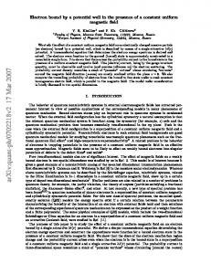

![arXiv:1712.00039v3 [cond-mat.quant-gas] 17 Mar 2018](https://m.moam.info/img/260x300/arxiv171200039v3-cond-matquant-gas-17-mar-2018_5c171988097c477b0d8b4644.jpg)


![0603416v1 [math.CV] 17 Mar 2006](https://m.moam.info/img/260x300/0603416v1-mathcv-17-mar-2006_5c9ce7b5097c47031d8b45a3.jpg)
![0511747v2 [math.RA] 17 Mar 2006](https://m.moam.info/img/260x300/0511747v2-mathra-17-mar-2006_5c64f5de097c476b448b4653.jpg)
![0303198v1 [math.AG] 17 Mar 2003](https://m.moam.info/img/260x300/0303198v1-mathag-17-mar-2003_5c3bcf06097c47aa258b4613.jpg)
![0403286v1 [math.DG] 17 Mar 2004](https://m.moam.info/img/260x300/0403286v1-mathdg-17-mar-2004_5c1b4e06097c47fe6d8b478e.jpg)
![0409129v2 [math.AG] 17 Mar 2010](https://m.moam.info/img/260x300/0409129v2-mathag-17-mar-2010_5c508121097c473b648b45cc.jpg)


![2203383 [math.GM] 22 Mar 2018](https://m.moam.info/img/260x300/2203383-mathgm-22-mar-2018_5c430eb8097c473c238b46cb.jpg)
![2201625 [math.GM] 20 Mar 2018](https://m.moam.info/img/260x300/2201625-mathgm-20-mar-2018_5c93971a097c471f4c8b4635.jpg)


