Ary Interpolating Subdivision Schemes - Semantic Scholar

Hindawi Publishing Corporation International Journal of Mathematics and Mathematical Sciences Volume 2013, Article ID 893414, 8 pages http://dx.doi.org/10.1155/2013/893414

Research Article Four-Point 𝑛-Ary Interpolating Subdivision Schemes Ghulam Mustafa and Robina Bashir Department of Mathematics, The Islamia University of Bahawalpur, Punjab, Bahawalpur 63100, Pakistan Correspondence should be addressed to Ghulam Mustafa; [email protected] Received 27 July 2013; Revised 27 September 2013; Accepted 27 September 2013 Academic Editor: Palle E. Jorgensen Copyright © 2013 G. Mustafa and R. Bashir. This is an open access article distributed under the Creative Commons Attribution License, which permits unrestricted use, distribution, and reproduction in any medium, provided the original work is properly cited. We present an efficient and simple algorithm to generate 4-point n-ary interpolating schemes. Our algorithm is based on three simple steps: second divided differences, determination of position of vertices by using second divided differences, and computation of new vertices. It is observed that 4-point n-ary interpolating schemes generated by completely different frameworks (i.e., Lagrange interpolant and wavelet theory) can also be generated by the proposed algorithm. Furthermore, we have discussed continuity, Hölder regularity, degree of polynomial generation, polynomial reproduction, and approximation order of the schemes.

1. Introduction In general, subdivision schemes can be divided into two categories: approximating and interpolating. For interpolating curve subdivision, new vertices are computed and added to the old polygons for each time of subdivision and the limit curve passes through all the vertices of the original control polygon. Interpolating subdivision schemes are more attractive than approximating schemes in computer aided geometric designs because of their interpolation property. In addition, the interpolation subdivisions are more intuitive to the users. Initial work on interpolating subdivision schemes was started by Dubuc [1]. Later on, Deslauriers and Dubuc [2] have introduced a family of schemes by using Lagrange polynomials indexed by the size of the mask and the arity. In [3], Dyn et al. have studied a family of interpolating schemes with mask size of four. Consequent to this, the research communities are interested in introducing higher arity schemes (i.e., ternary, quaternary, . . . , 𝑛-ary) which give better results and less computational cost. Lian [4] has constructed both the 2𝑚-point 𝑛-ary for any 𝑛 ≥ 2 and (2𝑚 + 1)-point 𝑛-ary for any odd 𝑛 ≥ 3 interpolatory subdivision schemes for curve design by using wavelet theory. Mustafa and Rehman [5] have presented general formulae for the mask of (2𝑏+4)-point 𝑛-ary interpolating and approximating schemes for any integer 𝑏 ≥ 0 and 𝑛 ≥ 2. These formulae

provide mask of higher arity schemes and generalize lower arity schemes. Mustafa et al. [6] have presented an explicit formula for the mask of odd points 𝑛-ary, for any odd 𝑛 ≥ 3, interpolating subdivision schemes. In [7], it has been proved that the large support and higher arity schemes may outperform than small support and lower arity schemes. Even though these schemes are not in practice. It has been suggested that the research on large support and higher arity schemes may continue. The multistage approach is very handy to construct subdivision schemes. This idea is variously used by others. Lane and Riesenfeld [8] have presented two fast subdivision algorithms for the evaluation of B-spline and Bernstein curves and surfaces. They have expressed new idea, in which, after a single duplication stage in which the number of control points is doubled by just taking each point twice, a sequence of smoothing operators is applied. Catmull and Clark [9] have used this technique to present the original description of subdivision in which each refinement is expressed in three stages. Zorin and Schröder [10] have considered the construction of an increasing sequence of alternating primal/dual quadrilateral subdivision schemes based on a simple averaging approach. Oswald and Schröder [11] used the same motif to generate families of subdivision schemes. Augsdörfer et al. [12] first describe the original 4-point binary subdivision scheme and then apply six variations on the scheme which are obtained by tuning the local stages

2

International Journal of Mathematics and Mathematical Sciences

in various ways, producing some interesting subdivision schemes all of which are improvements on the original. We generalize the same technique to build the family of fourpoint 𝑛-ary interpolating subdivision schemes. It is observed that 4-point 𝑛-ary interpolating schemes introduced by [2, 4] can also be constructed by our generalized technique, even though these schemes have been constructed by different frameworks. This paper is organized as follows: Section 2 presents some preliminary results. Section 3 consists of multistep algorithm which generates 4-point 𝑛-ary interpolating subdivision schemes. Analysis of two schemes is also presented in this section. In Section 4, Hölder regularity, polynomial generation, polynomial reproductions and approximation order of ternary and quaternary subdivision schemes have been discussed. Numerical examples and conclusion are presented in Section 5.

2. Preliminaries A general compact form of univariate 𝑛-ary subdivision scheme S [13] which maps polygon 𝑓𝑘 = {𝑓𝑖𝑘 }𝑖∈Z to a refined polygon 𝑓𝑘+1 = {𝑓𝑖𝑘+1 }𝑖∈Z is defined by 𝑓𝑖𝑘+1 = ∑ 𝑎𝑛𝑗−𝑖 𝑓𝑗𝑘 ,

𝑖 ∈ Z,

𝑗∈Z

The subdivision scheme 𝑆1 with Laurent polynomial 𝑎(1) (𝑧) is related to the scheme 𝑆 with Laurent polynomial 𝑎(𝑧) by the following theorem. Theorem 1 (see [14]). Let 𝑆 denote a subdivision scheme with Laurent polynomial 𝑎(𝑧) satisfying (5). Then there exists a subdivision scheme 𝑆1 with the property Δ𝑓𝑘 = 𝑆1 Δ𝑓𝑘−1 ,

𝑘 − 𝑓𝑖𝑘 ); 𝑖 ∈ Z}. where 𝑓𝑘 = 𝑆𝑘 𝑓0 and Δ𝑓𝑘 = {(Δ𝑓𝑘 )𝑖 = 𝑛𝑘 (𝑓𝑖+1 Furthermore, 𝑆 is a uniformly convergent if and only if (1/𝑛)𝑆1 converges uniformly to zero function for all initial data 𝑓0 , in the sense that 𝑘 1 lim ( 𝑆1 ) 𝑓0 = 0. 𝑘→∞ 𝑛

∑ 𝑎𝑛𝑗 = ∑ 𝑎𝑛𝑗+1 = ∑ 𝑎𝑛𝑗+2 = ⋅ ⋅ ⋅ = ∑ 𝑎𝑛𝑗+𝑛−1 = 1. 𝑗∈Z

𝑗∈Z

𝑗∈Z

(1)

{ 󵄨 󵄨 󵄨 󵄨 󵄨 󵄨 ‖𝑆‖∞ = max { ∑ 󵄨󵄨󵄨󵄨𝑎𝑛𝑗 󵄨󵄨󵄨󵄨 , ∑ 󵄨󵄨󵄨󵄨𝑎𝑛𝑗+1 󵄨󵄨󵄨󵄨 , ∑ 󵄨󵄨󵄨󵄨𝑎𝑛𝑗+2 󵄨󵄨󵄨󵄨 𝑗∈Z 𝑗∈Z {𝑗∈Z

󵄨 󵄨 lim sup 󵄨󵄨󵄨𝑓𝑖𝑘 − 𝑓 (𝑛−𝑘 𝑖)󵄨󵄨󵄨󵄨 = 0.

𝑘 → ∞𝑖∈𝑛𝑘 𝐼 󵄨

(3)

Obviously, 𝑓 = 𝑆 𝑓 . A symbol called Laurent polynomial 𝑎 (𝑧) = ∑ 𝑎𝑖 𝑧𝑖

(4)

𝑖∈Z

of the mask 𝑎 = {𝑎𝑖 : 𝑖 ∈ Z} plays an efficient role to analyze the convergence and smoothness of subdivision scheme. From (2) and (4) the Laurent polynomial of convergent subdivision scheme satisfies 𝑎 (𝛼𝑛𝑗 ) = 0,

𝑗 = 1, 2, . . . , 𝑛 − 1,

𝑎 (1) = 𝑛,

(5)

where 𝛼𝑛𝑗 = exp((2𝜋𝑖/𝑛)𝑗) are the 𝑛th root of unity. This condition guarantees the existence of a related subdivision scheme for the divided differences of the original control points and the existence of an associated Laurent polynomial 𝑎(1) (𝑧) = 𝑛𝑧𝑛−1 (

󵄩󵄩 𝐿󵄩 󵄩󵄩 { 󵄨 } 󵄨󵄨 󵄩󵄩 1 󵄨 ; 𝑖 = 0, 1, 2, . . . , 𝑛𝐿 − 1 , 󵄩󵄩( 𝑆𝛽 ) 󵄩󵄩󵄩 = max { ∑ 󵄨󵄨󵄨󵄨𝑏[𝛽,𝐿] 𝐿𝑗󵄨 󵄨 } 𝑖+𝑛 󵄩󵄩 𝑛 󵄩󵄩 󵄨 󵄨 󵄩 󵄩∞ {𝑗∈Z } (10) where 𝑏[𝛽,𝐿] (𝑧) =

∞ 0

1−𝑧 ) 𝑎 (𝑧) . 1 − 𝑧𝑛

(6)

(9)

󵄨 󵄨} , . . . , ∑ 󵄨󵄨󵄨󵄨𝑎𝑛𝑗+𝑛−1 󵄨󵄨󵄨󵄨} , 𝑗∈Z }

(2)

A subdivision scheme is uniformly convergent if for any initial data 𝑓0 = {𝑓𝑖0 : 𝑖 ∈ Z}, there exists a continuous function 𝑓 such that for any closed interval 𝐼 ⊂ R, it satisfies

(8)

The above theorem indicates that for any given scheme 𝑆, with the mask 𝑎 satisfying (2), we can prove the uniform convergence of 𝑆 by deriving the mask of (1/𝑛)𝑆1 and computing ‖((1/𝑛)𝑆1 )𝑖 ‖∞ for 𝑖 = 1, 2, 3 . . . , 𝐿, where 𝐿 is the first integer for which ‖((1/𝑛)𝑆1 )𝐿 ‖∞ < 1. If such an 𝐿 exists, then 𝑆 converges uniformly. Since there are “𝑛” rules for computing the values at the next refinement level, so we define the norm

where the set 𝑎 = {𝑎𝑖 : 𝑖 ∈ Z} of coefficients is called the mask at 𝑘th level of refinement. A necessary condition for the uniform convergence of subdivision scheme (1) is that 𝑗∈Z

(7)

𝑎𝛽 (𝑧) = (𝑛𝑧𝑛−1 ( = (𝑛𝑧𝑛−1 (

𝑗 1 𝐿−1 ∏𝑎𝛽 (𝑧𝑛 ) , 𝐿 𝑛 𝑗=0

1−𝑧 )) 𝑎𝛽−1 (𝑧) 1 − 𝑧𝑛 1−𝑧 𝛽 )) 𝑎 (𝑧) , 1 − 𝑧𝑛

(11) 𝛽 ⩾ 1.

Theorem 2 (see [13]). Let 𝑆 be the subdivision scheme with a characteristic ℧-polynomial 𝑎(𝑧) = 𝑚 ((𝑧𝑛 − 1)/(𝑛𝑧𝑛−1 (𝑧 − 1))) 𝑞(𝑧), 𝑞 ∈ ℧. If the subdivision scheme 𝑆𝑚 , corresponding to the ℧-polynomial 𝑞(𝑧), converges uniformly, then 𝑆∞ 𝑓0 ∈ 𝐶𝑚 (R) for any initial control polygon 𝑓0 . Corollary 3 (see [13]). If 𝑆 is a subdivision scheme of the form above and (1/𝑛)𝑆𝑚+1 converges uniformly to the zero function for all initial data 𝑓0 , then 𝑆∞ 𝑓0 ∈ 𝐶𝑚 (R) for any initial control polygon 𝑓0 .

International Journal of Mathematics and Mathematical Sciences p1 p2 b

z

1 n

2 n

···

pn−1

···

n−1 n

b

c

a

d

z

e

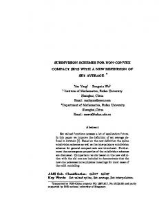
Figure 1: Labeling a sample control polygon. The newly inserted points between old vertices 𝑏 and 𝑐 are referred to as 𝑝1 , 𝑝2 ,. . ., 𝑝𝑛−1 , respectively.

The above Corollary 3 indicates that for any given 𝑛ary subdivision scheme 𝑆, we can prove 𝑆∞ 𝑓0 ∈ 𝐶𝑚 by first deriving the mask of (1/𝑛)𝑆𝑚+1 and then computing ‖((1/𝑛)𝑆𝑚+1 )𝑖 ‖∞ for 𝑖 = 1, 2, 3, . . . , 𝐿 (where 𝐿 is the first integer for which ‖((1/𝑛)𝑆𝑚+1 )𝐿 ‖∞ < 1). If such an 𝐿 exists, then 𝑆∞ 𝑓0 ∈ 𝐶𝑚 . Definition 4 (see [15]). For any subdivision scheme 𝑆𝑎 we denote by 𝜏 = 𝑎󸀠 (1)/𝑛 the corresponding parametric shift and attach the data 𝑓𝑖𝑙 for 𝑖 ∈ Z, 𝑙 ∈ N to the parameter values 𝑡𝑖𝑙 = 𝑡0𝑙 +

𝑖 𝑛𝑙

with 𝑡0𝑙 = 𝑡0𝑙−1 −

𝜏 . 𝑛𝑙

(12)

Theorem 5 (see [15]). A convergent subdivision scheme 𝑆𝑎 reproduces polynomials of degree 𝑑 with respect to the parameterizations (12) if and only if 𝑘−1

𝑎(𝑘) (1) = 𝑛∏ (𝜏 − 𝑙) , 𝑙=0

𝑗 = 1, 2, . . . , 𝑛 − 1

3

𝑎(𝑘) (𝛼𝑛𝑗 ) = 0,

p2

1 3

2 3

c

d

a

(ii) Determine the position of vertices by using divided differences. In 𝑛-ary subdivision scheme each segment is divided into 𝑛 subsegments at each refinement level. First point is inserted at the position 1/𝑛 and second point at the position 2/𝑛 and proceeding in the same way the (𝑛−1)-th point at the position (𝑛−1)/𝑛. By using divided differences 𝐷𝑏 and 𝐷𝑐 , we calculate the position of (𝑛 − 1)-th newly inserted points between two old vertices 𝑏 and 𝑐 by 𝐷𝑝𝑗 = (

𝑛−𝑗 𝑗 ) 𝐷𝑏 + ( ) 𝐷𝑐 , 𝑛 𝑛

𝑗 = 1, 2, 3, . . . , 𝑛 − 1. (15)

(iii) Computation new vertices. Finally, we calculate positions of new vertices 𝑝1 , 𝑝2 ,. . ., 𝑝𝑛−1 by using 𝐷𝑝1 , 𝐷𝑝2 ,. . ., 𝐷𝑝𝑛−1 , respectively, by 𝐷𝑝1 = 𝑝2 − 2𝑝1 + 𝑏, 𝐷𝑝𝑖 = 𝑝𝑖+1 − 2𝑝𝑖 + 𝑝𝑖−1 ,

where 𝛼𝑛𝑗 = exp((2𝜋𝑖/𝑛)𝑗), 𝑗 = 1, 2, . . . , 𝑛 − 1. Theorem 6 (see [16]). A convergent subdivision scheme 𝑆𝑎 that reproduces polynomial 𝜋𝑛 (set of polynomials at most degree 𝑛) has an approximation order of 𝑛 + 1.

e

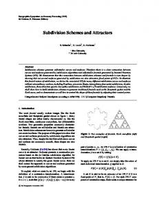
Figure 2: Labeling a sample control polygon. The newly inserted points between old vertices 𝑏 and 𝑐 are referred to as 𝑝1 and 𝑝2 , respectively.

(13)

for 𝑘 = 0, . . . , 𝑑,

p1

(16)

𝐷𝑝𝑛−1 = 𝑐 − 2𝑝𝑛−1 + 𝑝𝑛−2 , where 𝑖 = 2, 3, . . . , 𝑛 − 2. By solving, above set of equations, we get the position of new vertices 𝑝1 , 𝑝2 , . . . , 𝑝𝑛−1 .

3. Multistep Algorithm We construct 4-point 𝑛-ary interpolating subdivision schemes by using three-step algorithm instead of using Lagrange polynomial and wavelets theory, and so forth. These three steps are as follows. (i) Calculate second divided differences.

3.1. Examples. A 4-Point Ternary Interpolating Scheme. In ternary subdivision scheme each segment is divided into three subsegments at each refinement level. One point is inserted at the position 1/3 and another point at the position 2/3 (see Figure 2). For 𝑛 = 3 in (14), we get second divided differences 𝐷𝑏 and 𝐷𝑐 at points 𝑏 and 𝑐

At each old vertex compute the second divided difference 𝐷; that. is 𝐷𝑏 is the second divided difference at point 𝑏 and 𝐷𝑐 is the second divided difference at point 𝑐 (see Figure 1): 𝐷𝑏 =

𝑐 − 2𝑏 + 𝑎 , 𝑛2

𝑑 − 2𝑐 + 𝑏 𝐷𝑐 = , 𝑛2 where 𝑛 = 3, 4, . . ..

(14)

𝐷𝑏 =

𝑐 − 2𝑏 + 𝑎 , 9

(17)

𝑑 − 2𝑐 + 𝑏 𝐷𝑐 = . 9 For 𝑛 = 3 in (15), we get 𝐷𝑝𝑗 =

3−𝑗 𝑗 𝐷𝑏 + 𝐷𝑐 , 3 3

𝑗 = 1, 2.

(18)

4

International Journal of Mathematics and Mathematical Sciences p1

p2

p3

1 4

2 4

3 4

b

c

𝑓4𝑖𝑘+1 = 𝑓𝑖𝑘 ,

a

z

4-point quaternary interpolating scheme of Deslauriers and Dubuc

d

e

Figure 3: Labeling a sample control polygon. The newly inserted points between old vertices 𝑏 and 𝑐 are referred to as 𝑝1 , 𝑝2 , and 𝑝3 respectively.

𝑘+1 𝑓4𝑖+1 =−

𝑘+1 =− 𝑓4𝑖+2 𝑘+1 =− 𝑓4𝑖+3

By using (17), we get 𝐷𝑝1 = 𝐷𝑝2 =

(19)

𝑎 − 2𝑏 + 2𝑑 . 27

𝐷𝑝1 = 𝑝2 − 2𝑝1 + 𝑏,

𝑝2 =

𝑏 + 2𝑐 − 𝐷𝑝1 − 2𝐷𝑝2 3

𝑝2 =

Remark 7. By substituting 𝑛 ≥ 3 in (14)–(16), we get the mask of 4-point 𝑛-ary interpolating scheme generated by two different frameworks, that is, Lagrange interpolation [2] and wavelet theory [4]. In this paper, we propose alternative approach completely different from these approaches. In coming section, we discuss two existing schemes also produced by our framework.

, (21) .

3.2.1. Analysis of 4-Point Ternary Subdivision Scheme. The Laurent polynomial 𝑎(𝑧) for the scheme (23) is 𝑎 (𝑧) =

By using (19), we get 𝑝1 =

5 𝑘 35 𝑘 105 𝑘 7 𝑘 𝑓 + 𝑓 + 𝑓 − 𝑓 . 128 𝑖−1 128 𝑖 128 𝑖+1 128 𝑖+2

3.2. Analysis of Subdivision Schemes. Here we present the analysis of 4-point ternary and quaternary interpolating subdivision schemes. Analysis of other schemes can be done in a similar way.

This implies

3

(24)

(20)

𝐷𝑝2 = 𝑐 − 2𝑝2 + 𝑝1 .

2𝑏 + 𝑐 − 2𝐷𝑝1 − 𝐷𝑝2

1 𝑘 9 9 𝑘 1 𝑘 − 𝑓𝑖+2 , 𝑓𝑖−1 + 𝑓𝑖𝑘 + 𝑓𝑖+1 16 16 16 16

This scheme was also reconstructed by [4] in 2009.

2𝑎 − 3𝑏 + 𝑑 , 27

For 𝑛 = 3 in (16), we have

𝑝1 =

7 𝑘 105 𝑘 35 𝑘 5 𝑘 𝑓 + 𝑓 + 𝑓 − 𝑓 , 128 𝑖−1 128 𝑖 128 𝑖+1 128 𝑖+2

−5𝑎 + 60𝑏 + 30𝑐 − 4𝑑 , 81 −4𝑎 + 30𝑏 + 60𝑐 − 5𝑑 . 81

+ 60𝑧1 + 81 + 60𝑧−1 + 30𝑧−2

Using (11) for 𝑛 = 3, 𝛽 = 1, 2 and 𝐿 = 1, we get 𝑏[1,1] (𝑧) =

𝑓3𝑖𝑘+1 = 𝑓𝑖𝑘 , 5 𝑘 60 30 𝑘 4 𝑘 = − 𝑓𝑖−1 + 𝑓𝑖𝑘 + 𝑓𝑖+1 − 𝑓𝑖+2 , 81 81 81 81

𝑘+1 𝑓3𝑖+2

4 𝑘 30 60 𝑘 5 𝑘 = − 𝑓𝑖−1 + 𝑓𝑖𝑘 + 𝑓𝑖+1 − 𝑓𝑖+2 . 81 81 81 81

(25)

− 5𝑧−4 − 4𝑧−5 } .

(22)

Now 4-point ternary scheme can be written as

𝑘+1 𝑓3𝑖+1

1 {−4𝑧5 − 5𝑧4 + 30𝑧2 81

1 4 1 𝑎1 (𝑧) = − 𝑧5 − 𝑧4 3 81 81 +

5 3 26 2 29 1 26 5 𝑧 + 𝑧 + 𝑧 + + 𝑧−1 81 81 81 81 81

−

1 −2 4 −3 𝑧 − 𝑧 , 81 81

(23)

The above scheme was introduced by Deslauriers and Dubuc [2] in 1989 by using Lagrange interpolant. Later on, this scheme was also reconstructed by [4] by using wavelet theory. A 4-Point Quaternary Interpolating Scheme. In quaternary subdivision scheme each segment is divided into four subsegments at each refinement level. First, second and third points are inserted at the positions 1/4, 2/4, and 3/4, respectively (see Figure 3). For 𝑛 = 4 in (14)–(16), we get the following

𝑏[2,1] (𝑧) =

1 2 1 4 𝑎 (𝑧) = − 𝑧5 + 𝑧4 + 𝑧3 3 2 27 9 9

(26)

(27)

17 2 1 4 + 𝑧2 + 𝑧1 + − 𝑧−1 . 27 9 9 27 If 𝑆𝛽 is the scheme corresponding to 𝑎𝛽 (𝑧), then by (10) 󵄩󵄩 1 󵄩󵄩 󵄩󵄩 𝑆 󵄩󵄩 = max { ∑ 󵄨󵄨󵄨󵄨𝑏[𝛽,1] 󵄨󵄨󵄨󵄨 : 𝑖 = 0, 1, 2} , 󵄩󵄩 𝛽 󵄩󵄩 } { 󵄨󵄨 𝑖+3𝑗 󵄨󵄨 󵄩 3 󵄩∞ } {𝑗∈Z

𝛽 = 1, 2. (28)

International Journal of Mathematics and Mathematical Sciences Using (9), (26), and (27), we get 󵄨 󵄨 󵄨 󵄨 󵄨 󵄨 󵄨 󵄨 󵄨 󵄨 󵄨 󵄨 󵄩󵄩 1 󵄩󵄩 󵄩󵄩 𝑆 󵄩󵄩 = max {󵄨󵄨󵄨 −4 󵄨󵄨󵄨 + 󵄨󵄨󵄨 26 󵄨󵄨󵄨 + 󵄨󵄨󵄨 5 󵄨󵄨󵄨 , 󵄨󵄨󵄨 −1 󵄨󵄨󵄨 + 󵄨󵄨󵄨 29 󵄨󵄨󵄨 + 󵄨󵄨󵄨 −1 󵄨󵄨󵄨} , 󵄨󵄨 󵄨󵄨 󵄨󵄨 󵄨󵄨 󵄨󵄨 󵄨󵄨 󵄨󵄨 󵄨󵄨 󵄨󵄨 󵄨󵄨 󵄨󵄨 󵄨󵄨 󵄩󵄩 1 󵄩󵄩 󵄨 81 󵄨 󵄨 81 󵄨 󵄨 81 󵄨 󵄨 81 󵄨 󵄨 81 󵄨 󵄨 81 󵄨 󵄩 3 󵄩∞ 󵄩󵄩 1 󵄩󵄩 󵄨 󵄨 󵄨 󵄨 󵄨 󵄨 󵄨 󵄨 󵄨 󵄨 󵄩󵄩 𝑆 󵄩󵄩 = max {󵄨󵄨󵄨 −4 󵄨󵄨󵄨 + 󵄨󵄨󵄨 17 󵄨󵄨󵄨 + 󵄨󵄨󵄨 −4 󵄨󵄨󵄨 , 󵄨󵄨󵄨 1 󵄨󵄨󵄨 + 󵄨󵄨󵄨 2 󵄨󵄨󵄨} . 󵄩󵄩 2 󵄩󵄩 󵄨󵄨 󵄨󵄨 󵄨󵄨 󵄨󵄨 󵄨󵄨 󵄨󵄨 󵄨󵄨 󵄨󵄨 󵄨󵄨 󵄨󵄨 󵄩 3 󵄩∞ 󵄨 27 󵄨 󵄨 27 󵄨 󵄨 27 󵄨 󵄨 9 󵄨 󵄨 9 󵄨

Proof. The Laurent polynomial (25) of the scheme (23) can be written as 4

Remark 8. Similarly, we can prove that quaternary 4-point subdivision scheme is 𝐶1 .

4. Properties of Subdivision Schemes In this section, we show that how limit curve of 4-point ternary and 4-point quaternary subdivision schemes give response to initial polynomial data. For this we discuss Hölder regularity, degree of polynomial generation, polynomial reproduction and approximation order of the schemes (23) and (24). 4.1. Hölder Regularity. Hölder regularity is an extension of the notion of continuity which gives more information about any scheme. A function 𝜙 : 𝑅 → 𝑅 is defined to be regular of order 𝑦 + 𝛼 (for 𝑦 ∈ 𝑁0 and 0 < 𝜓 ≤ 1) if it is 𝑦 time continuously differentiable and 𝜙𝑦 is Lipschitz of order 𝛼 󵄨 󵄨󵄨 (𝑦) 󵄨󵄨𝜙 (𝑥 + ℎ) − 𝜙(𝑦) (𝑥)󵄨󵄨󵄨 ≤ 𝑐|ℎ|𝜓 (30) 󵄨 󵄨 for all 𝑥 and ℎ in 𝑅 and some constant 𝑐. According to Dyn and Levin [17] and Rioul [18], the Hölder regularity of subdivision scheme with symbol 𝑎(𝑧) can be computed in the following way. Let 𝑎(𝑧) = 𝑘 ((1 + 𝑧 + ⋅ ⋅ ⋅ + 𝑧𝑛−1 )/𝑛) 𝑏(𝑧), without loss of generality we can assume 𝑏0 , . . . , 𝑏𝑚 to be the nonzero coefficients of 𝑏(𝑧) and let 𝐵0 , 𝐵1 , . . . , 𝐵𝑚 be the 𝑚 × 𝑚 matrices with elements 𝑖, 𝑗 = 1, . . . , 𝑚,

Theorem 9. The Hölder regularity of scheme (23) is 𝑟 = 4 − log3 (11) = 1.8173.

(29)

As we see ‖(1/3)𝑆1 ‖∞ < 1, then by Theorem 1 the scheme is 𝐶0 . Similarly, ‖(1/3)𝑆2 ‖∞ < 1 then by Corollary 3 the scheme is 𝐶1 .

(𝐵𝑞 )𝑖𝑗 = 𝑏𝑚+𝑖−𝑛𝑗+𝑞 ,

5

𝑞 = 0, 1, . . . , 𝑚. (31)

Then the Hölder regularity is given by 𝑟 = 𝑘 − log𝑛 (𝜇), where 𝜇 is the joint spectral radius of the matrices 𝐵0 , 𝐵1 , . . . , 𝐵𝑚 , that is, 𝜇 = 𝜌 (𝐵0 , 𝐵1 , . . . , 𝐵𝑚 ) 󵄩1/𝑙 󵄩 = lim sup (max {󵄩󵄩󵄩󵄩𝐵𝑖𝑙 . . . 𝐵𝑖2 𝐵𝑖1 󵄩󵄩󵄩󵄩∞ : 𝑖𝑙 ∈ {0, 1}}) , 𝑙→∞ max {𝜌 (𝐵0 ) , . . . , 𝜌 (𝐵𝑚 )} ≤ 𝜌 (𝐵0 , . . . , 𝐵𝑚 ) 󵄩 󵄩 󵄩 󵄩 ≤ max {󵄩󵄩󵄩𝐵0 󵄩󵄩󵄩∞ , . . . , 󵄩󵄩󵄩𝐵𝑚 󵄩󵄩󵄩∞ } . (32) Since 𝜇 is bounded from below by the spectral radii and from above by the norm of the metrics 𝐵0 , 𝐵1 , . . .,𝐵𝑚 , then 󵄩 󵄩 󵄩 󵄩 max {𝜌 (𝐵0 ) , . . . , 𝜌 (𝐵𝑚 )} ≤ 𝜇 ≤ max {󵄩󵄩󵄩𝐵0 󵄩󵄩󵄩∞ , . . . , 󵄩󵄩󵄩𝐵𝑚 󵄩󵄩󵄩∞ } . (33)

1 + 𝑧 + 𝑧2 𝑎 (𝑧) = ( ) 𝑏 (𝑧) , 3

(34)

1 (−4 + 11𝑧 − 4𝑧2 ) . 𝑧5

(35)

where 𝑏 (𝑧) =

From (31) and (34), 𝑏0 = −4, 𝑏1 = 11, 𝑏2 = −4, 𝑘 = 4, 𝑚 = 2 and 𝑛 = 3, thus 𝑞 = 0, 1, 2, and then 𝐵0 , 𝐵1 , and 𝐵2 are the matrices with elements (𝐵0 )𝑖𝑗 = 𝑏2+𝑖−3𝑗 , (𝐵1 )𝑖𝑗 = 𝑏2+𝑖−3𝑗+1 ,

(36)

(𝐵2 )𝑖𝑗 = 𝑏2+𝑖−3𝑗+2 , where 𝑖, 𝑗 = 1, 2. This implies −4 0 𝐵0 = ( ), 11 0

11 0 𝐵1 = ( ), −4 0

−4 0 𝐵2 = ( ) . (37) 0 −4

From (33) and (37) we have max {4, 11, 4} ≤ 𝜇 ≤ max {11, 11, 4} .

(38)

Since the largest eigenvalue and the max-norm of the metrics are 11, so 𝑟 = 4 − log3 (11) = 1.8173.

(39)

Theorem 10. The Hölder regularity of scheme (24) is 𝑟 = 4 − log4 (24) = 1.7077. Proof. The Laurent polynomial 𝑎(𝑧) of scheme (24) can be written as 4

𝑎 (𝑧) = (

1 + 𝑧 + 𝑧2 + 𝑧3 ) 𝑏 (𝑧) , 4

(40)

where 𝑏 (𝑧) =

1 (−10 + 24𝑧 − 10𝑧2 ) . 𝑧7

(41)

From (31) and (40), 𝑏0 = −10, 𝑏1 = 24, 𝑏2 = −10, 𝑘 = 4, 𝑚 = 2 and 𝑛 = 4, thus 𝑞 = 0, 1, 2, and then 𝐵0 , 𝐵1 , and 𝐵2 are the matrices with elements (𝐵0 )𝑖𝑗 = 𝑏2+𝑖−4𝑗 , (𝐵1 )𝑖𝑗 = 𝑏2+𝑖−4𝑗+1 , (𝐵2 )𝑖𝑗 = 𝑏2+𝑖−4𝑗+2 ,

(42)

6


where 𝑖, 𝑗 = 1, 2. This implies −10 0 𝐵0 = ( ), 24 0

24 0 𝐵1 = ( ), −10 0

−10 0 𝐵2 = ( ). 0 −10 (43)

From (33) and (43) we have max {10, 24, 10} ≤ 𝜇 ≤ max {24, 24, 10} .

(44)

Thus the largest eigenvalue and the max-norm of the metrics are 24, so 𝑟 = 4 − log4 (24) = 1.7077.

(45)

Remark 11. It is generally observed that as we decrease the arity of the scheme the Hölder exponent increases. For example, Cashman et al. [19] have proved that the Hölder exponent for binary scheme is 2 while from above theorems we see that Hölder exponents for ternary and quaternary schemes are 1.8173 and 1.7077, respectively. Trivially, the Hölder exponent approaches to 1 for large arity scheme. 4.2. Polynomial Generation. The generation degree of a subdivision scheme is the maximum degree of polynomials that can potentially be generated by the scheme, provided that the initial data is chosen correctly. Suppose 𝑝0 is polynomial of degree 𝑑 of initial data 𝑓𝑖0 and symbol of the scheme is 𝑛−1 𝑑+1

𝑎 (𝑧) = (1 + 𝑧 + ⋅ ⋅ ⋅ + 𝑧

)

𝑏 (𝑧) ;

(46)

then the limit curve of the refined data 𝑓𝑖𝑘 at any level 𝑘 is polynomial of degree 𝑑. So the condition is necessary and sufficient for the scheme being able to generate polynomial of degree 𝑑. Theorem 12. The degree of polynomial generation of scheme (23) is 3. Proof. Since the Laurent polynomial 𝑎(𝑧) of the scheme (23) is 2 (3+1)

𝑎 (𝑧) = (1 + 𝑧 + 𝑧 )

𝑏 (𝑧) ,

1 (−4 + 11𝑧 − 4𝑧2 ) , (3)4 𝑧5

𝑏 (𝑧) ,

then degree of polynomial generation of scheme is 3.

𝑗 = 1, 2,

(51)

𝑗

for 𝑘 = 0, . . . , 3, 𝛼3 = exp((2𝜋𝑖/3)𝑗) and 𝜏 = 𝑎󸀠 (1)/3. Proof. By taking first derivative of (25) and substituting 𝑧 = 1 in it, we get 𝑎(1) (1) = 0.

(52)

This implies that 𝜏=

𝑎(1) (1) = 0. 3

(53)

So from (12), the scheme (23) has primal parametrization. For 𝑘 = 0, 𝑗 = 1, and from (25), we get 𝑎(0) (𝛼31 ) = 𝑎 (𝑒2𝜋𝑖/3 ) = 0.

(54)

Similarly, for 𝑗 = 1, 2 and 𝑘 = 0, 1, 2, 3 (𝑘 denotes the order of derivative) 𝑗

(55)

𝑘−1

(49)

where 1 𝑏 (𝑧) = (−10 + 24𝑧 − 10𝑧2 ) , (4)4 𝑧7

𝑙=0

(48)

Proof. Since the Laurent polynomial of (24) can be written as 𝑎 (𝑧) = (1 + 𝑧 + 𝑧 + 𝑧 )

𝑗

𝑎(𝑘) (𝛼3 ) = 0,

By (25), we get 𝑎(1) = 3. Also 3∏−1 𝑙=0 (0 − 𝑙) = 3, which implies (𝜏−𝑙). Similarly for 𝑘 = 1, 2, 3, we can easily that 𝑎(1) = 3∏0−1 𝑙=0 show that

Theorem 13. The degree of polynomial generation of scheme (24) is 3.

3 (3+1)

𝑘−1

𝑎(𝑘) (1) = 3∏ (𝜏 − 𝑙) ,

𝑎(𝑘) (𝛼3 ) = 0.

then degree of polynomial generation is 3.

2

Theorem 14. A convergent subdivision scheme (23) reproduces polynomials of degree 3 with respect to the parameterizations (12) if and only if

(47)

where 𝑏 (𝑧) =

4.3. Polynomial Reproduction and Approximation Order. The polynomial reproduction property has its own importance, as the reproduction property of the polynomials up to a certain degree 𝑑 implies that the scheme has 𝑑 + 1 approximation order. Polynomial reproduction of degree 𝑑 requires polynomial generation of degree 𝑑. For this, polynomial reproduction can be made from initial data which has been sampled from some polynomial function. In the view [15], the polynomial reproduction property of the proposed scheme can be obtained after having the parameterizations 𝜏 given in (12).

(50)

𝑎(𝑘) (1) = 3∏ (𝜏 − 𝑙) ,

(56)

𝑙=0

which completes the proof. Since scheme (23) reproduces polynomial of degree 3, so by using Theorem 6, we get the following theorem. Theorem 15. A 4-point ternary interpolating scheme (23) has an approximation order of 4. Proof of the following theorem is similar to the proof of Theorem 14.


(a) 4-point 2-ary

7

(b) 4-point 3-ary

(c) 4-point 4-ary

(d) 4-point 5-ary

(e) 4-point 6-ary

(f) 4-point 7-ary

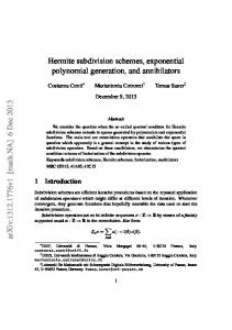
Figure 4: Comparison of the limit curves generated by proposed 4-point 2-ary, 3-ary, 4-ary, 5-ary, 6-ary, and 7-ary interpolating subdivision schemes at 1st subdivision level.

Theorem 16. A convergent subdivision scheme (24) reproduces polynomials of degree 3 with respect to the parameterizations (12) if and only if 𝑘−1

𝑎(𝑘) (1) = 4∏ (𝜏 − 𝑙) , 𝑙=0

𝑗

𝑎(𝑘) (𝛼4 ) = 0,

𝑗 = 1, 2, 3

(57)

𝑗

for 𝑘 = 0, . . . , 3, 𝛼4 = exp((2𝜋𝑖/4)𝑗) and 𝜏 = 𝑎󸀠 (1)/4.

by using imputation from Lagrange interpolation at four consecutive points [2]; therefore, 3-point ternary and 4-point quaternary schemes have polynomial reproduction of degree 3 and approximation properties are obvious (said by the referee). These schemes also have been generated by [4] using wavelet framework and by our algorithm, so by construction these schemes do no inherit these properties and that is only the reason to include the above theorems.

Again by Theorem 6, we get the following theorem. Theorem 17. A 4-point quaternary interpolating scheme (24) has an approximation order of 4. Remark 18. The considered schemes (i.e., 3-point ternary and 4-point quaternary) are exactly the same as obtained

5. Numerical Examples and Conclusion Six examples are depicted to show the usefulness of 4point 2-ary, 3-ary, 4-ary, 5-ary, 6-ary, and 7-ary interpolating subdivision schemes at 1st subdivision level in Figure 4. In this figure the control polygons are drawn by dotted lines

8 while the subdivision curves are drawn by solid lines. From Figure 4, it is clear that the initial polygon converges rapidly to limit curve as we increase the arity of the subdivision scheme. For many subdivision levels with any of these schemes the limit curves of the 𝑛-ary scheme with large 𝑛 may exhibit sharper singularities at the initial control points compared to the schemes with small 𝑛 (also mentioned by the referee). But if the initial control points come from noisy source, then 𝑛-ary scheme with large 𝑛 is the better choice. The scheme with small 𝑛 exhibit overfitting (see [7]). The main purpose to give comparison at first level is to provide the clear visual differences among the refined polygons produced by different schemes. In this paper, we have presented a multistep algorithm which generates 4-point 𝑛-ary interpolating subdivision schemes. We have also observed that the 4-point 𝑛-ary schemes generated by Lagrange polynomials and wavelet theory can also be generated by proposed multistep algorithm. Some significant properties like Hölder regularity, degree of polynomial generation, degree of polynomial reproduction, and approximation order have been also discussed in this paper.

Acknowledgments This work was supported by Indigenous Ph.D. Scholarship Scheme of HEC Pakistan. The authors would like to thank the referees for their helpful suggestions and comments which show the way to improve this work.

References [1] S. Dubuc, “Interpolation through an iterative scheme,” Journal of Mathematical Analysis and Applications, vol. 114, no. 1, pp. 185–204, 1986. [2] G. Deslauriers and S. Dubuc, “Symmetric iterative interpolation processes,” Constructive Approximation, vol. 5, no. 1, pp. 49–68, 1989. [3] N. Dyn, D. Levin, and J. A. Gregory, “A 𝑎-point interpolatory subdivision scheme for curve design,” Computer Aided Geometric Design, vol. 4, no. 4, pp. 257–268, 1987. [4] J.-A. Lian, “On 2𝑚-ary subdivision for curve design. III. (2𝑚 + 1)-point and (2𝑏+4)-point interpolatory schemes,” Applications and Applied Mathematics, vol. 4, no. 1, pp. 434–444, 2009. [5] G. Mustafa and N. A. Rehman, “The mask of 𝑛-point 𝑛-ary subdivision scheme,” Computing, vol. 90, no. 1-2, pp. 1–14, 2010. [6] G. Mustafa, J. Deng, P. Ashraf, and N. A. Rehman, “The mask of odd points 𝑛-ary interpolating subdivision scheme,” Journal of Applied Mathematics, vol. 2012, Article ID 205863, 20 pages, 2012. [7] G. Mustafa and I. P. Ivrissimtzis, “Model selection for the Dubuc-Deslauriers family of subdivision scheme,” in Proceedings of the 14th IMA Conference on Mathematics of Surfaces, University of Birmingham, Birmingham, UK, September2013. [8] J. M. Lane and R. F. Riesenfeld, “A theorical development for computer generation and display of piecewise polynomial surfaces,” IEEE Transaction on Pattern Analysis and Machine Intelligence, vol. 2, no. 1, pp. 35–46, 1980.

International Journal of Mathematics and Mathematical Sciences [9] E. Catmull and J. Clark, “Recursively generated B-spline surfaces on arbitrary topological meshes,” Computer Aided Geometric Design, vol. 10, no. 6, pp. 183–188, 1978. [10] D. Zorin and P. Schröder, “A unified framework for primal/dual quadrilateral subdivision schemes,” Computer Aided Geometric Design, vol. 18, no. 5, pp. 429–454, 2001, Subdivision algorithms (Schloss Dagstuhl, 2000). [11] P. Oswald and P. Schröder, “Composite primal/dual sprt(3) subdivision schemes,” Computer Aided Geometric Design, vol. 20, no. 3, pp. 135–164, 2003. [12] U. H. Augsdörfer, N. A. Dodgson, and M. A. Sabin, “Variations on the four-point subdivision scheme,” Computer Aided Geometric Design, vol. 27, no. 1, pp. 78–95, 2010. [13] N. Aspert, Non-linear subdivision of univariate signals and ´ discrete surfaces [EPFL Thesis], Ecole Polytechnique Fédérale de Lausanne, Lausanne, Switzerland, 2003. [14] M. F. Hassan and N. A. Dodgson, “Ternary and three-point univariate subdivision schemes,” in Curve and Surface Fitting, A. Cohen, J. L. Marrien, and L. L. Schumaker, Eds., pp. 199–208, Nashboro Press, Sant-Malo, France, 2002. [15] C. Conti and K. Hormann, “Polynomial reproduction for univariate subdivision schemes of any arity,” Journal of Approximation Theory, vol. 163, no. 4, pp. 413–437, 2011. [16] N. Dyn, Tutorials on Multiresolution in Geometric Modelling, Summer School Lecture Notes, Mathematics and Visualization, Springer, Berlin, Germany, 2002. [17] N. Dyn and D. Levin, “Subdivision schemes in geometric modelling,” Acta Numerica, vol. 11, pp. 73–144, 2002. [18] O. Rioul, “Simple regularity criteria for subdivision schemes,” SIAM Journal on Mathematical Analysis, vol. 23, no. 6, pp. 1544– 1576, 1992. [19] T. J. Cashman, K. Hormann, and U. Reif, “Generalized LaneRiesenfeld algorithms,” Computer Aided Geometric Design, vol. 30, no. 4, pp. 398–409, 2013.

Advances in

Decision Sciences

Advances in

Mathematical Physics Hindawi Publishing Corporation http://www.hindawi.com

Volume 2013

The Scientific World Journal Hindawi Publishing Corporation http://www.hindawi.com

Volume 2013

Mathematical Problems in Engineering Hindawi Publishing Corporation http://www.hindawi.com

Volume 2013

International Journal of

Combinatorics Hindawi Publishing Corporation http://www.hindawi.com

Volume 2013

Hindawi Publishing Corporation http://www.hindawi.com

Volume 2013

Journal of Applied Mathematics

Abstract and Applied Analysis Hindawi Publishing Corporation http://www.hindawi.com


Volume 2013

Volume 2013

Submit your manuscripts at http://www.hindawi.com Journal of Function Spaces and Applications

Discrete Dynamics in Nature and Society Hindawi Publishing Corporation http://www.hindawi.com


Volume 2013


Advances in

Journal of

Operations Research

Probability and Statistics



Stochastic Analysis

Differential Equations Hindawi Publishing Corporation http://www.hindawi.com

Volume 2013

ISRN Mathematical Analysis Hindawi Publishing Corporation http://www.hindawi.com


Volume 2013

ISRN Discrete Mathematics Volume 2013


Volume 2013


Volume 2013


Volume 2013

ISRN Applied Mathematics

ISRN Algebra Volume 2013


Volume 2013



Volume 2013

ISRN Geometry Volume 2013


Volume 2013