eJSE
Electronic Journal of Structural Engineering, 5 ( 2005)
International
Accelerograms for Dynamic Analysis under the New Australian Standard for Earthquake Actions Nelson Lam1, John Wilson2 and Srikanth Venkatesan3 1
2
Associate Professor and Reader, Dept. of Civil & Environmental Engineering, University of Melbourne, Vic 3010, Australia. Email:
[email protected] Professor of Civil Engineering, Faculty of Engineering and Industrial Sciences, Swinburne University of Technology, Vic 3122, Australia 3 Research Fellow, Department of Civil & Chemical Engineering, Royal Melbourne Institute of Technology, Vic 3000, Australia
Abstract The new Australian Standard for Earthquake Actions requires buildings exceeding 50 m in height and located in areas with hazard factor of Z ≥ 0.08 (which applies to most capital cities including Canberra, Sydney, Melbourne, Adelaide and Perth) to be designed for earthquake actions based on dynamic analyses. This paper presents a methodology for generating and using artificial accelerograms for obtaining site-specific design response spectra, which could be used for dynamic analyses. This time-history analysis approach of determining earthquake actions can result in more efficient designs in comparison with using response spectra specified by the Standard. An ensemble of accelerograms simulated for both rock and soil conditions are available in an electronic file named: “accelerograms for public access.xls” which can be downloaded free from the journal website for shared usage by all. The accelerogram file also contains listing of the baseline corrected displacement time-histories which are required for input into shaking table experiments and certain seismic simulation programs. Keywords : Artificial Accelerograms, Time-history, Earthquake, Seismic loading, Australia
10
Electronic Journal of Structural Engineering, 5 ( 2005)
1.
Introduction
This paper presents an ensemble of artificial accelerograms developed using stochastic simulations that are both appropriate for both the “hard rock” and “rock” conditions in Australia. The generated accelerograms have been used as input to SHAKE analyses (Idriss & Sun, 1992) for simulating ground motions on a soft soil site. Sample accelerograms simulated for both rock and soft soil conditions are available in electronic form for access through the journal website. The draft new Australian Standard for Earthquake Actions (AS/NZS 1170.4 Doc. D5212-5.1: June 2005) requires normal building structures exceeding 50m in height and located in areas with hazard factor, Z, of 0.08 to be designed in accordance with Earthquake Design Category III (EDC III) in which earthquake actions are to be determined by dynamic analyses. This applies generally to buildings exceeding 15-16 storeys in capital cities around Australia including Canberra, Sydney and Melbourne. For cities with slightly higher seismicity such as Adelaide and Newcastle, EDC III requirements are extended to buildings exceeding 25m in height (7-8 storeys) and founded on Class D and E sites. Dynamic analyses may take the form of response spectral analyses (RSA) or time-history analyses (THA). THA is considered to provide a more realistic representation of the actual response of the structure than RSA, particularly when the response is characterized by non-linear (inelastic) behaviour or significant torsional coupling behaviour. When time-history analyses are performed in engineering design, several representative ground motions should be used in order that the sensitivity of the response of the structure to random variations in the excitations can be tracked. The requirement for multiple analyses means that large number of accelerograms representing a range of conditions have to be sought. Accelerograms that were recorded locally in Australia were typically taken from small magnitude events, aftershocks, or from long epicentral distances. Near-field motions of engineering significance are very difficult to capture due to the infrequent, and seemingly random, characteristics of intraplate earthquakes. What is currently available is insufficient to meet seismic design requirements. Strong motion accelerograms that were recorded from outside the Australian continent may mis-represent local conditions even though the records could be taken from regions with similar levels of seismicity (eg. Central and Eastern North America). In countries with a paucity of strong motion data, like Australia, the use of accelerograms generated artificially by computer based on stochastic simulations has become a viable alternative for THA. The purpose of this paper is to present accelerograms that have been generated for engineering applications using program GENQKE that was developed at the University of Melbourne (Lam et al, 2000a; Lam, 1999). In view of the wide engineering readership of the paper, emphasis is on examining the peak ground velocity and response spectral properties of the accelerograms which are of direct engineering interest. Detailed coverage of the seismological aspects of the subject are beyond the scope of this paper but specific details on seismological modelling for Australian conditions are given in Lam et al (2003). The simulation methodology used has been well established and review articles on this subject can be found in the literature (eg. Lam et al 2000a). It is shown that separate modelling is required for (i) “hard rock” conditions of Western and Central Australia and (ii) “rock” conditions of Eastern Australia. Accelerograms simulated for rock outcrop conditions in both these regions are presented in Section 2. Response spectra of the generated accelerograms have also been calculated. Results were averaged and presented systematically for a range of magnitude and distances. Samples are shown in Section 3. The peak 11
Electronic Journal of Structural Engineering, 5 ( 2005)
ground velocity behaviour inferred from the calculated response spectra were then compared against the well known Gaull’s model which was developed from analyses of Intensity data of local historical events recorded in Australia. The verification analyses also compared data collected from the 1989 Newcastle earthquake against computer simulations. Results of the comparative analyses provide support to the claim that the generated accelerograms are generally consistent with local conditions (refer Section 4). Further verification analyses addressing the long-period behaviour of the accelerograms are presented in Section 5. Finally, accelerograms simulated for a Class D (deep or soft soil) site have been obtained using the program SHAKE and artificial accelerograms generated for rock conditions as input bedrock motion (refer Section 6). Response spectra for both rock and soft soil conditions are presented for comparison with the design response spectra stipulated by the new Australian Standard for earthquake actions.
2.
Artificial Accelerograms
Sample acceleration time-histories on “rock” conditions characteristics of Eastern Australia are presented in Figures 1 & 2 to show the increase in the duration of the accelerogram with earthquake magnitude and distance in accordance with the relationship defined in Lam et al (2000a). These accelerograms can be modified to represent the filtering effects of soil sediments using well-established standard procedures in which bedrock accelerograms are used as the input motion. Ground shaking could be significantly prolonged on soft soil sites increasing the risk of damage to structures.
2
M6 R=30km
Acceleration (m/sec/sec)
1.5 1 0.5 0 -0.5 -1 -1.5 -2 0
2
4
6
8
10
12
14
16
18
20
Time (sec) Figure 1
Time-histories of simulated accelerograms for earthquake scenario of M6 R=30km on “rock” characteristics of Eastern Australian conditions
12
Electronic Journal of Structural Engineering, 5 ( 2005)
0.8
M7 R=100km
Acceleration (m/sec/sec)
0.6 0.4 0.2 0 -0.2 -0.4 -0.6 -0.8 -1 0
2
4
6
8
10
12
14
16
18
20
Time (sec) Figure 2
Time-histories of simulated accelerograms for earthquake scenario of M7 R=100km on “rock” characteristics of Eastern Australian conditions
3. Response Spectra 3.1
Sensitivity study on sample size
Initially, the response spectrum of an individual simulated accelerogram was calculated. This response spectrum based on a single accelerogram was then compared with the average of 3, 6 and 18 accelerograms. Results of this comparative study are shown in Figures 3a – 3d for a Magnitude M=6, R=30 km earthquake. The irregular appearance of the response spectrum based on a single simulation is clearly noticeable, indicating a significant bias at certain periods. It is the opinion of the authors that a minimum of 4-6 randomly generated accelerograms has to be included in the analyses to effectively suppress the biases (as evidenced by the smoothness of the averaged response spectra associated with larger sample sizes).
3.2
Response spectra of accelerograms simulated for Eastern Australia
Eighteen random simulations have been produced for each earthquake scenario defined by a magnitude-distance (M-R) combination for the “rock” conditions of Eastern Australia. A response spectrum was then calculated for each simulation and results were averaged. A selection of the averaged response spectra are presented in Figures 4a -4c.
13
Electronic Journal of Structural Engineering, 5 ( 2005)
Response Spectral Velocity (m/sec)
1 Individual Simulation
0.1
0.01 0.01
0.1
1
10
Natural Period (sec) (a) Individual simulation
Response Spectral Velocity (m/sec)
1 Average of 3
0.1
0.01 0.01
0.1
1
10
Natural Period (sec) (b) Average of 3 simulations Figure 3. Sample size comparison of averaged response spectra 14
Electronic Journal of Structural Engineering, 5 ( 2005)
Response Spectral Velocity (m/sec)
1 Average of 6
0.1
0.01 0.01
0.1
1
10
Natural Period (sec) (c) Average of 6 simulations
Response Spectral Velocity (m/sec)
1 Average of 18
0.1
0.01 0.01
0.1
1
10
Natural Period (sec) (d) Average of 18 simulations Figure 3. Sample size comparison of averaged response spectra (cont’d) 15
Electronic Journal of Structural Engineering, 5 ( 2005)
3.3
Response spectra of accelerograms simulated for Western and Central Australia
Eighteen random simulations have also been produced for each earthquake scenario defined by a magnitude-distance (M-R) combination for the “hard rock” conditions of Western and Central Australia. A response spectrum has been calculated for each simulation and results averaged. The averaged response spectra are presented systematically in Figures 5a -5c.
Response Spectral Velocity (m/sec)
1
M5.5 R=30km M6 R=30km M6.5 R=30km M7 R=30km
RSV - Eastern Australia (R=30km)
0.1
0.01 0.01
0.1
1
10
Natural Period (sec) (a) R= 30 km
Response Spectral Velocity (m/sec)
1
M5.5 R=60km M6 R=60km M6.5 R=60km M7 R=60km
RSV - Eastern Australia (R=60km) 0.1
0.01
0.001 0.01
0.1
1
10
Natural Period (sec)
16
Electronic Journal of Structural Engineering, 5 ( 2005)
(b) R= 60 km Figure 4. Response Spectra of accelerograms simulated for Eastern Australia
Response Spectral Velocity (m/sec)
1 M7 R=100km
RSV - Eastern Australia ( R=100km) 0.1
0.01
0.001 0.01
0.1
1
10
Natural Period (sec) (c) R= 100 km Figure 4. Response Spectra of accelerograms simulated for Eastern Australia (cont’d) An important parameter of engineering interests characterising each of the response spectra is the notional averaged peak ground velocity (PGV), which is defined herein as the highest point on the averaged velocity response spectrum divided by 1.8 (based on the recommendations of Wilson & Lam, 2003 citing the work of Somerville et al, 1998). Note, the actual PGV can be some 10-15% lower than the notional PGV. This notional averaged PGV is summarised in Table 1 below for each M-R combination. Table 1 PGV (mm/sec) of simulated motions for Eastern Australia Distance\Magnitud M5.5 M6 M6.5 e 10 km 132 242 20 km 58 109 180 30 km 36 66 109 45 km 21 38 63 60 km 16 29 49 80 km 39 100 km
M7
172 102 84 67 52
17
Electronic Journal of Structural Engineering, 5 ( 2005)
Response Spectral Velocity (m/sec)
1 M5.5 R=30km M6 R=30km M6.5 R=30km M7 R=30km
RSV - Western Australia (R=30km)
0.1
0.01 0.01
0.1
1
10
Natural Period (sec) (a) R= 30 km
18
Electronic Journal of Structural Engineering, 5 ( 2005)
Response Spectral Velocity (m/sec)
1 M5.5 R=60km M6 R=60km M6.5 R=60km M7 R=60km
RSV - Western Australia (R=60km) 0.1
0.01
0.001 0.01
0.1
1
10
Natural Period (sec) (b) R= 60 km Figure 5. Response Spectra of accelerograms simulated for Western & Central Australia
Response Spectral Velocity (m/sec)
1 M7 R=100km
0.1
RSV - Western Australia ( R=100km)
0.01
0.001 0.01
0.1
1
10
Natural Period (sec) (c) R= 100 km 19
Electronic Journal of Structural Engineering, 5 ( 2005)
Figure 5. Response Spectra of accelerograms simulated for Western & Central Australia (cont’d) The notional averaged peak ground velocity is also summarised in Table 2 below (as done for Eastern Australia). It is noted that the PGV’s of accelerograms simulated for Eastern Australia are significantly higher than those simulated for Western & Central Australia for the same magnitude-distance (M-R) combinations. Table 2 PGV (mm/sec) of simulated motions for Western & Central Australia Distance\Magnitude M5.5 M6 M6.5 M7 10 km 77 126 20 km 34 58 95 30 km 21 36 60 97 45 km 12 22 37 61 60 km 11 20 34 57 80 km 30 51 100 km 42
4.
Comparisons with Instrumented and Intensity Data
Sections 4 and 5 are concerned with benchmarking simulated accelerograms and their response spectra and demonstrating their accuracies. Response spectra recorded from a few small to moderate magnitude earthquakes occurring in central Australia and Eastern Canada have been compared with those simulated using program GENQKE. Modelling has been relatively straightforward in such environment given that frequency contents of seismic waves radiated from the source of the earthquake is not significantly modified in the transmission of waves through these stable continental interior regions of “hard rock” conditions. Consequently, good agreement has been found between computer simulations and field measurements (Lam et al, 2000b,c). Good simulation accuracies have also been demonstrated with case studies involving long distance earthquakes that affected Singapore, India etc. (refer Chandler & Lam, 2004). However, earthquake case studies that can be used to verify the accuracies of the presented simulation methodology is generally limited and comparisons have only been made on ad-hoc basis. A systematic approach to benchmarking simulated accelerograms is to compare their ground motion parameters (such as PGV’s) with predictions by existing empirical models (eg. Hutchinson et al, 2003). In Australia, attenuation modelling with instrumented data has only been undertaken very recently in Western Australia by Allen et al (2004). Attenuation modelling was based wholly on Modified Mercalli Intensity (MMI) data reported on iso-seismal maps of local historical earthquake events. A macro-seismic attenuation model was developed by Gaull et al (1990) in accordance with such data. The proposed attenuation relationship in terms of MMI for Eastern and Western & Central Australia is represented by equation (1a) and (1b) respectively. MMI = 1.5 M - 3.9 log R + 3.9 MMI = 1.5 M - 3.2 log R + 2.2
(1a) (1b)
A separate attenuation relationship has been developed for Northeastern Australia (Queensland region) which has been found to be intermediate between that of Western and Southeastern 20
Electronic Journal of Structural Engineering, 5 ( 2005)
Australia. In this study, the conditions of Southeastern Australia (where the major capital cities of Canberra, Sydney and Melbourne are located) is taken to apply to the whole of Eastern Australia. The modelled MMI values have been translated into the respective notional peak ground velocities (PGV's) based on the well known conversion relationship of equation (2). 2MMI = 7/5 PGV (mm/sec)
(2)
Since the predicted PGV values were originally based on observations of damage in historical earthquakes, the predictions are meant to be for common (or "average") site conditions, and not specifically for rock sites, or hard rock sites, unlike seismological models used for simulating artificial earthquake accelerograms. The PGV's obtained from the simulated accelerograms were then correlated with the PGV's calculated from the Gaull's model as shown in Figure 6a and 6b for rock and hard rock conditions respectively. The ratio between the two sets of data is the implied amplification factors of an "average" site. The implied average site factor is shown to be constrained at around 1.5-1.6 which is compared to the amplification factor of 1.4 stipulated by the new Draft Australian Standard for Class C sites. Note, Class C site is described as "shallow soil" site and is taken as the common site class of average conditions consistent with the definition of the Earthquake Intensity. This reasonable agreement in the predicted amplification factor of a common site supports the use of the simulated accelerograms for seismic risk analyses in both regions of Australia. The suitability of alternative attenuation models in representing Australian conditions could be tested using a similar approach.
21
Electronic Journal of Structural Engineering, 5 ( 2005)
PGV's from Gaull's Model (mm/sec)
200
1:1.5 1:2
150
1:1.5 1:1
100
50
0 0
50
100
150
200
PGV 's of Simulated Motions (mm/sec) (a) Eastern Australia
PGV's from Gaull's Model (mm/sec)
200
1:1.62
1:2 150 1:1.5
1:1 100
50
0 0
50
100
150
200
PGV's of Simulated Motions (mm/sec) (b) Western & Central Australia Figure 6. Peak ground velocities of simulated motions versus predictions by Gaull's Model The notional PGV estimated for an M5.5 earthquake is 132 mm/sec at R=10 km and 58 mm/sec at R=20 km as shown in Table 1. The PGV at 15km is approximately 90 -100 mm/sec by linear interpolation. An Intensity on the Modified Mercalli scale in the order of VII can be inferred for rock (or very stiff) sites from the calculated PGV based on equation (2). This earthquake 22
Electronic Journal of Structural Engineering, 5 ( 2005)
scenario is comparable to the 1989 earthquake which struck the city of Newcastle on the eastern coast of New South Wales and resulted in 11 deaths and over 2 billion dollar of damage. The inferred Intensity value is in agreement with what is shown on the Iso-seismal map of the event on the western part of the city (Melchers, 1990). 400 y = 1.67x R2 = 0.944
PGV mm/sec - Gaull(EA)
350
1:2 1:1.5
300
1:1
250
1:1.67
200 150 100 50 0 0
50
100
150
200
250
300
350
400
PGV mm/sec - Gaull (WA) (a) Gaull’s Model
PGV mm/sec - Simulations (EA)
400
y = 1.76x R2 = 0.97
350
1:2
300
1:1.5 250
1:1
200
1:1.76
150 100 50 0 0
50
100
150
200
250
300
350
400
PGV mm/sec - Simulations (WA) (b) Simulations Figure 7 Crustal factors inferred from regional differences The differences in the PGV’s predicted for the two regions of Australia provide indications of the extent of crustal modifications (given that there are negligible crustal modifications in hard 23
Electronic Journal of Structural Engineering, 5 ( 2005)
rock conditions of Western & Central Australia). Thus, a crustal factor can be inferred from the ratio of the notional PGV estimated for Eastern Australia and that for Western & Central Australia. This ratio was calculated for every M-R combinations based on the Gaull’s model (Figure 7a) and the simulated accelerograms (Figure 7b). A mean crustal factor of 1.67 was inferred from the Gaull’s model. This is compared to a mean crustal factor of 1.76 obtained similarly from the simulated accelerograms.
5.
Velocity-Displacement corner period behaviour
An effective way to characterize the long-period (up to 5 sec) behaviour of earthquake ground motions is to calculate the corner period which defines the transition between the velocitycontrolled and displacement-controlled sections of the response spectrum (Lam et al, 2000c; Lam & Chandler, 2005). The calculations may be based on equation (3).
Tcorner = 2π
RSD5 sec RSD5 sec = 2π RSVmax 1.8 PGV
(3)
During the 1990's, the Australian Geological Survey Organisation (AGSO) undertook a detailed study of 13 accelerograms measured at rock sites from reverse thrust fault events with magnitude ranging from 5.4 - 6.6 (Somerville et al, 1998). Records were normalised to a peak ground velocity (PGV) of 50 mm/sec, and the proposed normalised design response spectrum is shown below in Figure 8. The corner period of the averaged spectrum is shown to be around 0.7 sec.
m /s e
10 0m m
100 10 m /s e c2
90mm/sec 10 m m
/se c2
10
1 0.01
Tcorner 0.7sec 0. 1m /se c2
*results normalised to PGV=50mm/sec
m m
1. 8
10
1m
RSAmax=1.8m/sec2 RSVmax=90mm/sec RSDmax=10mm
Normalised RSV(mm/sec)
1000
c2
The long-period behaviour of the accelerograms simulated in this study (for both Western and Eastern Australia) has been checked by calculating the corner periods for individual earthquake scenarios and compared with the benchmark model of Somerville, et al., (1998) as shown in Figure 8. Results of the comparison are shown in Figure 9 for earthquake scenarios at the reference hypocentral distance of 30 km. The magnitude dependent behaviour of the corner frequency was identified in the study by Lam et al (2000c) from the simulation motions. The comparison of Figure 9 once again shows good agreement between the simulated motions and the recorded motions as represented by the model of Somerville et al (1998). Recognizing this, the design response spectra stipulated by the new Australian Standard for earthquake actions has the corner period set conservatively at 1.5 sec representing a major earthquake event in the order of magnitude M=7.
0.1
1m
1.0
m
10
Natural Period (sec)
Figure 8. Normalised Empirical Spectrum Model of Somerville
24
Electronic Journal of Structural Engineering, 5 ( 2005)
2 Simulations for Western Australia
1.8
Simulations for Eastern Australia
Corner Period (sec)
1.6
Somerville's Model
1.4 1.2 1 0.8 0.6 0.4 0.2 0 5
5.5
6
6.5
7
7.5
Magnitude Figure 9 Corner periods at velocity-displacement transition
6.
Simulations for a deep or soft soil site
Accelerograms presented in the earlier parts of this paper were based on hard rock and rock conditions which can be described as site category Class A and B respectively according to the new Australian Standard for earthquake actions (AS/NZS 1170.4 Doc. D5212-5.1: June 2005). A more onerous sub-soil condition is considered in this section. A borehole record representing such condition is shown in Figure 10a. The shear wave velocity profile of the soil sedimentary layers, totaling 55m in thickness as shown in Figure 10b, was inferred from the borehole record using relationships recommended in Lam & Wilson (1999). The site natural period is estimated accordingly at around 1 second which suggests a Class D site category. Site response analyses were undertaken using program SHAKE (Idriss & Sun, 1992) based on a multitude of earthquake scenarios with varying magnitude-distance (M-R) combinations producing PGV of about 60 mm/sec on the rock surface (which is consistent with a hazard factor, Z, of 0.08 as stipulated by the Standard for Melbourne, Sydney and Canberra). It is shown in Figures 11a-11d that the more critical scenario for soil response pertains to the one with a larger earthquake magnitude while the rock PGV is kept constant. Thus, the soil response spectrum simulated for the M=7 scenario (Figure 11d) is most critical and hence conservative for design applications. Simulations based on the M=6.5 scenario (Figure 11c) seem to match best with the design response spectrum stipulated by the Standard. Thus, the acceleration time-history corresponding to the M=6.5 earthquake scenario is recommended for use in time-history analyses for design purposes for site sub-soil conditions comparable to that shown in Figure 10. 25
Electronic Journal of Structural Engineering, 5 ( 2005)
For other sub-soil conditions, accelerograms should be simulated using a site response analysis program such as SHAKE and representative rock accelerograms as input information.
ground surface 9m
Silty Sand
15.5 m
Soft clay
2.5 m
Silty Sand
5.5 m
Clay
2m
Silty Sand
5m 15 m
Clay Silty Sand Rock SWV = 1000 m/s
Figure 10 (a) Borehole log Shear Wave Velocity (m/sec) 0
100
200
300
400
0 10
Depth (m)
20 30 40 50 60
(b) Shear wave velocity profile Figure 10. (a) Borehole log and (b) Shear wave velocity profile for example Soft Soil (class D) site 26
Electronic Journal of Structural Engineering, 5 ( 2005)
An example “rock outcrop” accelerogram associated with the design scenario of M=6.5 and R= 45km is shown (in Figure 12a) along with the accelerogram simulated for the surface of the soft soil site (in Figure 12b). An electronic file containing accelerograms simulated for this earthquake scenario for different site classes can be accessed through the journal website. The two simulated acceleration time-histories have similar amplitude but very different frequency contents, which is evident from the corresponding ensemble averaged response spectra presented in the different formats in Figures 13a-d. Explanations of the response spectrum formats are given in Wilson & Lam (2003). The most critical displacement demand is shown to occur at the site natural period as indicated by the “corner point” on the velocity spectrum (Figure 13b), a single dominant peak on the displacement spectrum (Figure 13c) and a “nose” shaped feature on the ADRS diagram (Figure 13d). The vertical arrow shown along with the “broken line” on the velocity and displacement response spectra highlights a maximum soil amplification ratio in the order of about 1: 4 at this critical period. This displacement amplification behaviour is not evident in the response spectrum presented in the conventional acceleration format of Figure 13a (noting that peaks appearing on the acceleration spectrum are positioned differently to the peak on the displacement spectrum). It is noted that the seismic displacement demand can become more onerous than that presented in this section if the site natural period is higher than 1 second. The borehole log and corresponding shear wave velocity profile for an example Class C site is also shown in Appendix A. That particular site has a shallower soil profile than the example Class D site of Figure 10. However, the site specific velocity response spectrum may “locally“ exceed that of a Class D site at the site natural period of 0.6 sec (which is most onerous for a Class C site). Accelerograms simulated for this site Class C model are also available for access through the journal website.
1000
Response Spectral Velocity (mm/sec)
M=5.5 ; R=20 km-GENQKE
Soil-M=5.5;R=20 km-GENQKE-SHAKE
Code-Rock
Code-Site-D
100
10 0.1
1
10
Natural Period (sec)
(a) M=5.5, R= 20 km 27
Electronic Journal of Structural Engineering, 5 ( 2005)
Response Spectral Velocity (mm/sec)
1000 M=6 ; R=30 km-GENQKE Soil-M=6;R=30 km-GENQKE-SHAKE Code Site Class B (Rock) Code-Site Class D (Soft Soil)
100
10 0.1
1
10
Natural Period (sec)
(b) M=6, R= 30 km
Response Spectral Velocity (mm/sec)
1000 M=6.5 ; R=45 km-GENQKE Soil-M=6.5;R=45 km-GENQKE-SHAKE Code Site Class B (Rock) Code-Site Class D (Soft Soil)
100
10 0.1
1
10
Natural Period (sec)
(c) M=6.5, R= 45 km
28
Electronic Journal of Structural Engineering, 5 ( 2005)
1000
Response Spectral Velocity (mm/sec)
M=7 ; R=80 km-GENQKE Soil-M=7;R=80 km-GENQKESHAKE Code Site Class B (Rock)
100
10 0.1
1
10
Natural Period (sec)
(d) M=7, R= 80 km Figure 11. Velocity response spectra simulated for rock and soft soil conditions for comparison with design response spectra stipulated by the new Australian Standard (cont’d) 2.5
Acceleration (m/sec/sec)
2 1.5 1 0.5 0 -0.5 -1 -1.5 -2 -2.5 0
2
4
6
8
10
12
14
16
18
20
Time (sec) (a) Class B Rock site
29
Electronic Journal of Structural Engineering, 5 ( 2005)
2.5
Acceleration (m/sec/sec)
2 1.5 1 0.5 0 -0.5 -1 -1.5 -2 -2.5 0
2
4
6
8
10
12
14
16
18
20
Time (sec) (b) Class D Soft Soil site Figure 12 Accelerograms simulated for M=6.5 R=45 km earthquake scenario spectra 0.4 Rock
Soft Soil
Response Spectral Acceleration (g)
0.35 0.3 0.25 0.2 0.15 0.1 0.05 0 0
1
2
3
4
5
6
Natural Period (sec)
(a) Acceleration response spectra Figure 13 Rock and soft soil spectra in different formats 30
Electronic Journal of Structural Engineering, 5 ( 2005)
Rock Soft Soil Corner point
100
10 0.1
1
10
Natural Period (sec) (b) Velocity response spectra 45 Rock 40
Response Spectral Displacement (mm)
Response Spectral Velocity (mm/sec)
1000
Soft Soil
35 30 25 20 15 10 5 0 0
1
2
3
4
5
6
Natural period (sec)
(c) Displacement response spectra
31
Electronic Journal of Structural Engineering, 5 ( 2005)
0.4 Rock
Response Spectral Acceleration (g)
0.35
Soft Soil
0.3 0.25 0.2 0.15 0.1 0.05 0 0
10
20 30 40 Response Spectral Displacement (mm)
50
(d) Acceleration-Displacement Response Spectrum (ADRS) Diagrams Figure 13. Rock and soft soil velocity response spectra in different formats (cont’d)
7.
Conclusion
Artificial accelerograms have been generated by computer based on stochastic simulations of the seismological model. Separate modelling is required for (i) “hard rock” conditions of Western and Central Australia and (ii) “rock” conditions of Eastern Australia. An important parameter of engineering interests characterising each of the response spectra is the notional averaged peak ground velocity (PGV), which is defined herein as the highest point on the averaged velocity response spectrum divided by 1.8. The PGV's obtained from the simulated accelerograms have been correlated with the PGV's calculated from Gaull's model. The ratio between the two sets of data, which is shown to be constrained at around 1.5-1.6, is close to the amplification factor stipulated for a Class C (or "average") site consistent with the definition of the Earthquake Intensity. The differences in the PGV’s predicted for the two regions of Australia provide indications of the extent of crustal modifications. A mean crustal factor of 1.67 was inferred from the Gaull’s model. This compares favourably with a mean crustal factor of 1.76 obtained from the simulated accelerograms. The velocity-displacement transition behaviour of the accelerograms simulated in this study has been checked by calculating the corner periods for individual earthquake scenarios and comparing with the benchmark model of Somerville. The comparison shows good agreement between the simulated motions and the Somerville model in terms of their corner period behaviour. The design response spectra stipulated by the new Australian Standard for earthquake 32
Electronic Journal of Structural Engineering, 5 ( 2005)
actions have the corner period set conservatively at 1.5 second representing a major earthquake event in the order of magnitude M=7. The borehole record of a soft soil site with 55m deep sedimentary layers and site natural period of around one second (subsoil category Class D) was subject to site response analyses using the program SHAKE. The most critical displacement demand calculated for the soil surface is indicated by the “corner point” on the velocity spectrum and the single dominant peak on the displacement spectrum. The most critical scenario when PGV is kept constant pertains to the one with a larger earthquake magnitude. The M=6.5 scenario seems to provide the best match with the design response spectrum stipulated by the new Standard. Therefore, acceleration time-histories corresponding to this earthquake scenario are recommended for use in time-history analyses for design purposes, and are available in an electronic format for access through the journal web address. For sub-soil conditions which are more onerous than that shown in Figure 10 (eg. site natural period exceeding 1 second), accelerograms should be simulated using a site response analysis program such as SHAKE and with accelerograms simulated for a Class A or B site as the input bedrock excitations.
7.
References
Allen, T, Dhu, T., Cummins, P., Schneider, J. and Gibson, G., (2004). Some empirical relations for attenuation of ground-motion spectral amplitudes in southwestern western Australia, Procs. of the Australian Earthquake Engineering Society Conference, Mt. Gambier, south Australia. Paper no. 11. AS/NZS 1170.4 Draft no.DR04303 (2004) Structural Design Actions - Part 4 Earthquake Actions, sub-committee BD006-11, Standards Australia. Chandler, A.M. and Lam, NT.K. (2004). An attenuation model for distant earthquakes, Earthquake Engineering and Structural Dynamics. John Wiley & Sons Ltd., Vol.33(2):183-210. Draft AS/NZS 1170.4 (2005). Draft for Public Comment Australian Standard for Structural Design Actions, Part 4 : Earthquake Actions in Australia. Document No. D5212-5.1 issued in June 2005.
Gaull, B.A. Michael-Leiba, M.O. and Rynn, J.M.W. (1990). Probabilistic earthquake risk maps of Australia. Australian Journal of Earth Sciences 37:169-187. Hutchinson, G.L. Lam, N.T.K. and Wilson, J. (2003). Determination of earthquake loading and seismic performance in intraplate regions, Progress in Structural Engineering and Materials, John Wiley & Sons Ltd., Vol.5:181-194. Idriss, I.M. and Sun, J.I. (1992). Users Manual for SHAKE-91, sponsored by National Institue of Standards and Technology, Maryland USA and Dept. of Civil & Environmental Engineering., University of California, Davis, USA. Lam, N.T.K. and Wilson, J.L. (1999). Estimation of the site natural period form a borehole record, Australian Journal of Structural Engineering. Inst. of Engineers 1(3), 179-199.
Lam, N.T.K. (1999). Program GENQKE User;s Manual, Civil & Environmental Engineering, University of Melbourne Lam, N.T.K Wilson, J.L. and Hutchinson, G.L. (2000a). Generation of synthetic earthquake accelerograms using seismological modeling: a review, J Earthquake Engineering, Vol 4, No 3, pp 321-354. Lam, N.T.K. Wilson, J.L. Chandler, A.M. and Hutchinson, G.L.(2000b). Response Spectral Relationships for rock sites derived from the Component Attenuation Model, Earthquake Engineering and Structural Dynamics, 29(10),14571489. Lam, N.T.K. Wilson, J.L. Chandler, A.M. and Hutchinson, G.L. (2000c). Response Spectrum Modelling for Rock Sites in Low and Moderate Seismicity Regions Combining Velocity, Displacement and Acceleration Predictions, Earthquake Engineering and Structural Dynamics, Vol.29(10), 1491-1526. Lam, N.T.K. Sinadinovski, C. Koo, R.C.H. and Wilson, J.L. (2003). Peak ground velocity modelling for Australian earthquakes. International Journal of Seismology and Earthquake Engineering 5(2), 11-22. Lam, N.T.K. and Chandler, A.M. (2005). Peak Displacement Demand in Stable Continental Regions, Earthquake Engineering and Structural Dynamics. John Wiley & Sons Ltd, Vol.34: 1047-1072. Melchers, R.E. (1990). Editor. Newcastle Earthquake Study. Report of the Institution of Engineers, Australia.
33
Electronic Journal of Structural Engineering, 5 ( 2005) Somerville, M. McCue, K. and Sinadinovski, C. (1998) Reponse Spectra Recommended for Australia, Australian Structural Engineering Conference, Auckland, 1998: 439-444. Wilson, J.L. and Lam, N.T.K. (2003). A recommended earthquake response spectrum model for Australia, Australian Journal of Structural Engineering. Inst. of Engineers 5(1), 17-27.
34
Electronic Journal of Structural Engineering, 5 ( 2005)
Appendix A – Borehole log and shear wave velocity profile for a Class C site Ground surface 2m
Sand
9.5 m
Clay
3.5 m
Sand
6m
Clay
2m
Sand Rock
Figure A1 Borehole log of an example Class C site
Shear wave velocity (m/sec) 0
100
200
300
400
0
Depth (m)
5
10
15
20
25
Figure A2 Shear wave velocity profile for an example Class C site
35